Sparse Non negative Matrix Language Modeling

Sparse Non-negative Matrix Language Modeling

Joris Pelemans Google Inc. ESAT, KU Leuven [email protected]

Noam Shazeer Google Inc. [email protected]

Ciprian Chelba Google Inc.

[email protected]

Abstract

We present Sparse Non-negative Matrix (SNM) estimation, a novel probability estima-tion technique for language modeling that can efficiently incorporate arbitrary features. We evaluate SNM language models on two cor-pora: the One Billion Word Benchmark and a subset of the LDC English Gigaword cor-pus. Results show that SNM language models trained withn-gram features are a close match

for the well-established Kneser-Ney models. The addition of skip-gram features yields a model that is in the same league as the state-of-the-art recurrent neural network language models, as well as complementary: combin-ing the two modelcombin-ing techniques yields the best known result on the One Billion Word Benchmark. On the Gigaword corpus further improvements are observed using features that cross sentence boundaries. The computational advantages of SNM estimation over both max-imum entropy and neural network estimation are probably its main strength, promising an approach that has large flexibility in combin-ing arbitrary features and yet scales gracefully to large amounts of data.

1 Introduction

A statistical language model estimates probability values P(W) for strings of wordsW in a

vocabu-laryV whose size can be in the tens or hundreds of

thousands and sometimes even millions. Typically the stringW is broken into sentences, or other

seg-ments such as utterances in automatic speech recog-nition, which are often assumed to be conditionally independent; we will assume thatW is such a

seg-ment, or sentence.

Estimating full sentence language models (Rosen-feld et al., 2001) is computationally hard if one

seeks a properly normalized probability model1_over

strings of words of finite length in V∗. A simple

and sufficient way to ensure proper normalization of the model is to decompose the sentence prob-ability according to the chain rule and make sure that the end-of-sentence symbol</S> is predicted with non-zero probability in any context. With

W =wN

1 =w1, . . . , wN we get:

P(w₁N) =

N

Y

k=1

P(w_k|wk₁−1) (1)

Since the parameter space ofP(wk|wk₁−1)is too large, the language model is forced to put the con-textw₁k−1into anequivalence classdetermined by a functionΦ(w₁k−1). As a result,

P(wN₁ )∼=

N

Y

k=1

P(w_k|Φ(wk₁−1)) (2)

Research in language modeling consists of find-ing appropriate equivalence classifiersΦand meth-ods to estimateP(w_k|Φ(wk₁−1)). Arguably the most successful paradigm in language modeling uses the

n-gramequivalence classification, that is, defines

Φn-gram(w1k−1) .

=wk−n+1, wk−n+2, . . . , wk−1

Once the formΦ(w₁k−1)is specified, only the prob-lem of estimating P(w_k|Φ(wk₁−1)) from training data remains.

In order to outperform the n-gram equivalence

class, one must find a way to leverage long-distance context. This can be done explicitly, e.g. by combin-ing multiple arbitrary features (Rosenfeld, 1994), or implicitly as is the case for the current state of the art

1_{In some practical systems the constraint on using a properly}

normalized language model is side-stepped at a gain in model-ing power and simplicity, see e.g. Chen et al. (1998).

329

recurrent neural network language models (Mikolov, 2012). Unfortunately, either method comes at a large computational cost which makes training and evaluation on a large corpus impractical.

In this paper we present a novel probability esti-mation technique, called Sparse Non-negative Ma-trix (SNM) estimation. Although SNM estimation is a general approach that can be applied to many problems, its efficient combination of arbitrary fea-tures makes it particularly interesting for language modeling. We demonstrate this by training models with variable-lengthn-gram features and skip-gram

features to incorporate long-distance context. The paper is organized as follows: Section 2 dis-cusses work that is related to SNM which is de-scribed in Section 3. We then present a complex-ity analysis in Section 4 and experimental results on two English corpora in Sections 5 and 6. We end with conclusions and future work in Section 7.

2 Related Work

2.1 Neural networks

Recently, neural networks (NN) (Bengio et al., 2003; Emami, 2006; Schwenk, 2007), and in par-ticular recurrent neural networks (RNN) (Mikolov, 2012; Sundermeyer et al., 2012) have shown ex-cellent performance in language modeling (Chelba et al., 2014). RNNLMs have two main advantages overn-gram language models: 1) they learn a

low-dimensional continuous vector representation for words which allows them to discover fine-grained similarities between words; 2) they are capable of modeling dependencies that span over longer dis-tances, i.e. they can extend the context past the n -gram window. Their main disadvantage however is that they take a long time to train and evaluate.

2.2 Feature-based models

Another popular method to leverage long-distance context is Maximum Entropy (ME) (Rosenfeld, 1994). ME is interesting because it can mix dif-ferent types of features extracted from large context windows, e.g.n-gram, skip-gram, bag-of-word and

syntactic features. Unfortunately it suffers from the same drawback as neural networks, as we will see in Section 2.4.

The above-mentioned features can also be used in

other ways, e.g. Chelba and Jelinek (2000) use a left-to-right syntactic parser to identify long-distance de-pendencies (at sentence level), whereas approaches such as Bellegarda (2000) leverage latent semantic information (at document level). Tan et al. (2012) in-tegrate both syntactic and topic-based modeling with

n-grams in a unified approach.

2.3 Skip-grams

The type of long-distance features that we incor-porate into our SNMLMs are skip-grams (Huang et al., 1993; Ney et al., 1994; Rosenfeld, 1994), which can effectively capture dependencies across longer contexts. We are not the first to highlight this effectiveness; previous such results were reported in Singh and Klakow (2013). Recently, Pickhardt et al. (2014) also showed that a backoff generaliza-tion using single skips yields significant perplexity reductions. We note though that our SNMLMs are trained by mixing single as well as longer skips, combining both in one model. More fundamentally, the SNM model parameterization and method of es-timation are completely original, as far as we know. In our approach, a skip-gram feature extracted from the contextw₁k−1is characterized by the tuple

(r, s, a)where:

• rdenotes the number of remote context words

• sdenotes the number of skipped words

• adenotes the number of adjacent context words

relative to the target wordwk being predicted. The

window size of a feature extractor then corresponds to r +s +a. For example, in the sentence <S> The quick brown fox jumps over the lazy dog </S>a(1,2,3)skip-gram feature for the target worddogis:

[brown skip-2 over the lazy] For performance reasons, it is recommended to limitsand to limit either(r+a)or bothrands.

We configure the skip-gram feature extractor to produce all features F, defined by the equivalence class Φ(wk₁−1), that meet constraints on the mini-mum and maximini-mum values for:

We also allow the option of not including the ex-act value ofsin the feature representation; this may

help with smoothing by sharing counts for various skip features. The resulting tied skip-gram features will look like:

[curiosity skip-* the cat] In order to build a good probability estimate for the target wordwkin a contextw1k−1we need a way

of combining an arbitrary number of skip-gram fea-tures, which do not fall into a simple hierarchy like regularn-gram features. The standard way to

com-bine such predictors is ME, but it is computationally hard. The proposed SNM estimation on the other hand is capable of combining such predictors in a way that is computationally easy, scales up grace-fully to large amounts of data and as it turns out is also very effective from a modeling point of view.

2.4 Log-linear models

Neural networks and ME are related in the sense that for both modelsP(w_k|Φ(w₁k−1)) takes the follow-ing form:

P(wk|Φ(w₁k−1)) = _Xexp(ˆywk)

t0_∈V

exp(ˆyt0)

(3)

where theyˆt0 are the unnormalized log-probabilities for each potential target wordt0 and depend on the

model in question. For a ME model with featuresF, they can be represented as follows:

ˆ

y=xTM (4)

wherexis the word feature activation vector andM

is a|F|×|V|feature weight matrix. Theyiˆ of neural networks on the other hand are computed as follows:

ˆ

y=g(xTH)W (5)

where g(_·) is the activation function of the hidden layer (typically a tanhor sigmoid) and W andH

are weight matrices for the output and hidden layer respectively. Feed-forward and recurrent neural net-works differ only in their input vectorsx: in a feed-forward neural network,xis a concatenation of the

input features whereas in a recurrent neural network,

xis a concatenation of the input word with the pre-vious hidden state. Because of their shared log-linearity, training and evaluating these models be-comes computationally complex.

Although log-linear models have been shown to perform better than linear models (Klakow, 1998), their performance is also hampered by their com-plexity and we will show in the rest of the paper that a linear model can in fact compete with the state of the art when trained with variable-lengthn-gram and

skip-gram features combined.

3 Sparse Non-negative Matrix Estimation

3.1 Linear model

Contrary to neural networks and ME, SNM language models do not estimate P(wk|Φ(wk₁−1)) in a log-linear fashion, but are in fact log-linear models:

P(w_k|Φ(w₁k−1)) = yˆwk

X

t0_∈V ˆ

yt0

(6)

whereˆyis defined as in Eq. (4).

Like ME however, SNM uses featuresF that are

predefined and arbitrary, e.g.n-grams, skip-grams,

bags of words, syntactic features, ... The features are extracted from the left context ofwk and stored

in a feature activation vectorx = Φ(wk₁−1), which is binary-valued, i.e. xf represents the presence or

absence of the feature with indexf.

In what follows, we represent the target wordwk

by a vectory, which is a one-hot encoding of the

vo-cabularyV:yt= 1fort=wk,yt= 0otherwise. To

further simplify notation, we will not make the dis-tinction between a feature or target and its index, but rather denote both of them byf andt, respectively.

Theyˆt0 in SNM are computed in the same way as ME, using Eq. (4), whereMis a_{|F| × |V|} feature

weight matrix, which is sparse and non-negative.

Mf t is indexed by feature f and target t and

de-notes the influence of feature f in the prediction

of t. Plugging Eq. (4) into Eq. (6), we can

de-rive the complete form of the conditional distribu-tionP(y_|x) =P(w_k|Φ(w₁k−1))in SNMLMs:

P(y_|x) = (x

T_M) wk

P

t0_∈V(xTM)t0

=

P

f0_∈Fxf0Mf0wk

P

t0_∈V

P

f0_∈Fxf0Mf0t0

=

P

f0_∈Fxf0M_f0_wk

P

As required by the denominator in Eq. (7), this computation also involves summing over all the present features for the entire vocabulary. However, because of the linearity of the model, we can pre-compute the row sumsP_t0_∈VMf0_t0 for eachf0 and store them together with the model. This means that the evaluation can be done very efficiently, since the remaining summation involves a limited number of terms: even though the amount of features|F|

gath-ered over the entire training data is potentially huge, the amount of active, non-zero features for a given

x is small. For example, for SNM models using

variable-lengthn-gram features, the maximum num-ber of active features isn; in our experiments with a

large variety of skip-grams, it was around 100. Notice that this precomputation is not possible for the log-linear ME which is otherwise similar, be-cause the sum over all features does not distribute outside the sum over all targets in the denominator:

P(y_|x) = exp(

P

f0_∈Fxf0M_f0_wk)

X

t0_∈V

exp(X

f0_∈F

xf0M_f0_t0)

(8)

This is a huge difference and essentially makes SNM a more efficient model at runtime.

3.2 Adjustment function and meta-features

We let the entries of M be a slightly modified or

adjustedversion of the relative frequencies:

Mf t =eA(f,t) Cf t

Cf∗ (9)

where A(f, t) is a real-valued function, dubbed the adjustment function(to be defined below), and

C is a feature-target count matrix, computed over

the entire training corpus T. Cf t denotes the

co-occurrence count of featuref and target t, whereas Cf∗denotes the total occurrence count of featuref, summed over all targetst0.

An unadjusted SNM model, where A(f, t) = 0, is a linear mixture of simple feature modelsP(t_|f) with uniform mixture weights. The adjustment func-tion enables the models to be weighted by the rela-tive importance of each input feature and, because it also parameterized byt, takes into account the cur-rent target. The function is computed by a linear model on binarymeta-features(Lee et al., 2007):

A(f, t) =θ_·h(f, t) (10)

where h(f, t) is the meta-feature vector extracted from the feature-target pair(f, t).

Estimating weights θk on the meta-feature level

rather than the input feature level enables similar in-put features to share weights which improves gener-alization. We illustrate this by an example.

Given the word sequence the quick brown fox, we extract the following elementary meta-features from the 3-gram feature the quick brownand the targetfox:

• feature identity:[the quick brown]

• feature type: 3-gram

• feature count:Cf∗

• target identity:fox

• feature-target count:Cf t

We also allow conjunctions of (single or multi-ple) elementary meta-features to form more com-plex meta-features. This explains the absence of the feature-target identity (and others, see Appendix A) in the above list: it is represented by the conjunc-tion of the feature and target identities. The result-ing meta-features enable the model to share weights between, e.g. all 3-grams, all 3-grams that have tar-getfox, etc. Although these conjunctions may in theory overrideCf t/Cf∗in Eq. (9), keeping the rel-ative frequencies allows us to train the adjustment function on part of the data (see also Section 3.4).

We apply smoothing to all of the count meta-features: since count meta-features of the same order of magnitude carry similar information, we group them so they can share weights. We do this by bucketing the count meta-features according to their (floored) log₂ value. As this effectively puts the lowest count values, of which there are many, into a different bucket, we optionally introduce a sec-ond (ceilinged) bucket to assure smoother transi-tions. Both buckets are then weighted according to thelog₂fraction lost by the corresponding rounding operation. Pseudocode for meta-feature extraction and count bucketing is presented in Appendix A.

value modulo the pre-defined size(θ). We do not prevent collisions, which has the potentially unde-sirable effect of tying together the weights of differ-ent meta-features. However, as was previously ob-served by Mikolov et al. (2011), when this happens the most frequent meta-feature will dominate the fi-nal value after training, which essentially boils down to a form of pruning. Because of this, the model performance does not strongly depend on the size of the hash table. Note that we only apply hashing to the meta-feature weights: the adjusted and raw relative frequencies are stored as SSTables (Sorted String Table).

3.3 Model estimation

Although it is in principle possible to use regularized maximum likelihood to estimate the parameters of the model, a gradient-based approach would end up with parameter updates involving the gradient of the logof Eq. (7) which works out to:

∂logP(y|x)

∂A(f, t) =xfMf t

yt

ˆ

ywk

− X1

t0_∈V ˆ

yt0

(11)

For the complete derivation, see Appendix B. The problem with this gradient is that we need to sum over the entire vocabularyV in the denominator. In

Eq. (7) we could get away with this by precomput-ing the row sums, but here the sums change after each update. Instead, we were inspired by Xu et al. (2011) and chose to use an independent binary pre-dictor for each word in the vocabulary during esti-mation. Our approach however differs from Xu et al. (2011) in that we do not use|V|Bernoullis, but|V|

Poissons2_{, using the fact that for a large number of}

trials a Bernoulli with smallpis well approximated

by a Poisson with smallλ.

If we consider each yt0 in y to be Poisson dis-tributed with parameter yˆt0, the conditional proba-bilityPPois(y|x)is given by:

PPois(y|x) = Y

t0_∈V ˆ

yyt0

t0 e−yˆt0

yt0! =

Y

t0_∈V ˆ

yyt0

t0 e−ˆyt0 (12)

2_{We originally chose Poisson so we could apply the model}

to tasks with outputsyt >1. More recent experiments using a

multinomial loss can be found in Chelba and Pereira (2016).

and the gradient of the log-probability works out to:

∂logPPois(y|x)

∂A(f, t) =xfMf t

yt

ˆ

ywk

−1

(13)

For the complete derivation, see Appendix C. The parametersθ of the adjustment function are

learned by maximizing the Poisson log-probability, using stochastic gradient ascent. That is, for each feature-target pair(f, t)we compute the gradient in Eq. (13) and propagate it to the meta-feature weights

θk by multiplying it with ∂A(f, t)/∂θk = hk. At

theNthoccurrence of feature-target pair(f, t), each weightθkis updated using the propagated gradient,

weighted by a learning rateη:

θk,N ←θk,N−1+η∂N(f, t) (14)

where∂N(f, t)is a short-hand notation for theNth

gradient with respect toθk.

Rather than using a single fixed learning rate, we use AdaGrad (Duchi, 2011) which uses a separate adaptive learning rateηk,N for each weightθk,N:

ηk,N =

γ

q

∆0+PN_n=1∂n(f, t)2

(15)

where γ is a constant scaling factor for all

learn-ing rates and∆0 is an initial accumulator constant.

Basing the learning rate on historical information tempers the effect of frequently occurring features which keeps the weights small and as such acts as a form of regularization.

3.4 Optimization and leave-one-out training

Each feature-target pair (f, t) constitutes a training example where examples with yt = 0 are called

negative and others positive. Using the short-hand notations T = |T |, F = |F| and V = |V|, this means that the training data consists of approxi-matelyT F(V ₋1)negative and onlyT F positive training examples. If we examine the two terms of Eq. (13) separately, we see that the first term

xfMf t_yˆyt

wk depends onyt which means it becomes

zero for all the negative training examples. The sec-ond term−xfMf t however does not depend onyt

this, the vast amount of updates required for the neg-ative examples makes the update algorithm compu-tationally too expensive.

To speed up the algorithm we use a heuristic that allows us to express the second term as a function of yt, essentially redistributing the updates for the

numerous negative examples to the fewer positive training examples. Appendix D shows that for batch training this has the same effect if run over the entire corpus. We note that for online training this is not strictly correct, sinceMf tchanges after each update.

Nonetheless, we found this to yield good results as well as seriously reducing the computational cost. After applying the redistribution, the online gradient that is applied to each training example becomes:

∂logPPois(y|x)

∂A(f, t) =xfytMf t

1 ˆ

ywk

− C_Cf∗ f t

(16)

which is non-zero only for positive training exam-ples, hence making training independent of the size of the vocabulary.

One practical way to further prevent overfitting and adapt the model to a specific task is to use held-out data, i.e. compute the count matrix C on the

training data and estimate the parameters θ on the

held-out data. Unfortunately, since the aggregated gradients in Eq. (16) tie the updates to the counts

Cf∗ andCf t in the training data, they can’t

differ-entiate between held-out and training data, which means that the meta-feature weights can’t be tuned specifically to the held-out data. Experiments in which we tried to use the held-out counts instead did not yield good results, presumably because we are violating the redistribution heuristic.

Rather than adding a regularizer on the meta-feature weights, we instead opted for leave-one-out training. With the notationA(f, t, Cf∗, Cf t)

reflect-ing the dependence of the adjustment function on feature and feature-target counts, the gradient under leave-one-out training becomes:

xfyt

( 1

ˆ

y+wk

−1)M_{f t}+−Cf∗−Cf t Cf t

M_{f t}−

(17)

whereM_{f t}−,M_{f t}+andyˆ+

wk are defined as follows:

M_{f t}− =eA(f,t,Cf∗−1,Cf t) Cf t

Cf∗−1

M_{f t}+ =eA(f,t,Cf∗−1,Cf t−1)Cf t−1

Cf∗−1 ˆ

y_w+_k = (xTM+)wk

The full derivation can be found in Appendix E. We note that in practice, it often suffices to use only a subset of the training examples for leave-one-out training, which has the additional advantage of speeding up training even further.

4 Complexity analysis

Besides their excellent results, RNNs have also been shown to scale well with large amounts of data with regards to memory and accuracy (Williams et al., 2015). Compared to n-gram models which

grow huge very quickly with only modest improve-ments, RNNs take up but a fraction of the memory and exhibit a near linear reduction in log perplex-ity withlogtraining words. Moreover, a larger hid-den layer can yield more improvements, whereasn

-gram models quickly suffer from data sparsity. The problem with RNNs however is that they are compu-tationally complex which makes training and evalua-tion slow. A standard Elman network (Elman, 1990) with hidden layer of sizeH trained on a corpus of

sizeT with vocabulary of sizeV has complexity

IT(H2+HV) (18)

whereI indicates the number of iterations. Several

attempts have been made to reduce training time, fo-cusing mostly on reducing the large factorsT orV:

• vocabulary shortlisting (Schwenk and Gauvain,

2004)

• subsampling (Schwenk and Gauvain, 2005; Xu et al., 2011)

• class-based (Goodman, 2001b; Morin and Ben-gio, 2005; Mikolov et al., 2011)

• noise-contrastive estimation (Gutmann and

Hyv¨arinen, 2012; Chen et al., 2015)

do not sufficiently speed up training. The class-based implementation for example, still has a train-ing computational complexity of:

IT(H2+HC+CVC) (19)

whereCindicates the number of classes andVCthe

variable amount of words in a class. Although this is a significant reduction in complexity, the dominant termIT H2_{is still large. The same applies to}

noise-contrastive estimation.

As was shown in Mikolov et al. (2011), a Max-imum Entropy model can be regarded as a neural network with direct connections for the features, i.e. it has no hidden layers. The model uses the same softmax activation at its output and its complexity therefore also depends on the size of the vocabulary:

IT(F+V) (20)

whereF+ F denotes the number of active

fea-tures. To achieve state-of-the-art results this model is often combined with an RNN, which yields a total complexity of:

IT(H2+HV +F+V) (21)

The computational complexity for training SNM models on the other hand is independent ofV:

T F++IT0F+Θ+ (22)

whereΘ+ is the number of meta-features for each

of the F+ input features. The first term is related

to counting features and feature-target pairs and the second term to training the adjustment model on a subset T0 of the training data. If we

com-pare an SNMLM with typical values of F+≈100 andΘ+<40, to the RNNLM configurations with H= 1024 in Chelba et al. (2014) and Williams et al. (2015), we find that training comes at a reduced complexity of at least two orders of magnitude.

A even more striking difference in complexity can be seen at test time. Whereas the complexity of a class-based RNN for a single test step is propor-tional toH2+HC+CVC, testing SNMLMs is linear

inF+because of the reasons outlined in Section 3.1.

5 Experiment 1: 1B Word Benchmark Our first experimental setup used the One Billion Word Benchmark3 _{made available by Chelba et al.}

(2014). It consists of an English training and test set of about 0.8 billion and 159658 tokens, respec-tively. The vocabulary contains 793471 words and was constructed by discarding all words with count below 3. OOV words are mapped to an<UNK> to-ken which is also part of the vocabulary. The OOV rate of the test set is 0.28%. Sentence order is ran-domized.

All of the described SNM models are initialized with meta-feature weights θk = 0 which are

up-dated using AdaGrad with accumulator ∆0 = 1

and scaling factorγ = 0.02over a single epoch of 30M training examples. The hash table for the meta-features was limited to 200M entries as increasing it yielded no significant improvements.

5.1 N-gram experiments

In the first set of experiments, we used all variable-lengthn-gram features that appeared at least once in

the training data up to a given length. This yields at most nactive features: one for each m-gram of length0 ≤m < nwherem = 0corresponds to an

empty featurewhich is always present and produces the unigram distribution. The number of features is smaller thannwhen the context is shorter thann−1 words (near sentence boundaries) and during evalua-tion where ann-gram that did not occur in the train-ing data is discarded.

When trained using these features, SNMLMs come very close to n-gram models with

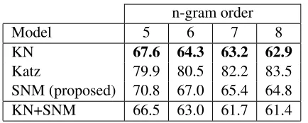
interpo-lated Kneser-Ney (KN) smoothing (Kneser and Ney, 1995), where no count cut-off was applied and the discount does not change with the order of the model. Table 1 shows that Katz smoothing (Katz, 1987) performs considerably worse than both SNM and KN. KN and SNM are not very complementary as linear interpolation with weights optimized on the test data only yields an additional perplexity reduc-tion of about 1%. The difference between KN and SNM becomes smaller when we increase the size of the context, going from 5% for 5-grams to 3% for 8-grams, which indicates that SNMLMs might be better suited to a large number of features.

n-gram order

Model 5 6 7 8

KN 67.6 64.3 63.2 62.9

Katz 79.9 80.5 82.2 83.5

SNM (proposed) 70.8 67.0 65.4 64.8

KN+SNM 66.5 63.0 61.7 61.4

Table 1: Perplexity results on the 1B Word Benchmark for Kneser-Ney (KN), Katz and SNMn-gram models of

different order.

Model PPL

SNM5-skip (non-grams) 69.8 +n-grams = SNM5-skip 54.2

+ KN5 56.5

SNM5-skip + KN5 53.6

Table 2: Perplexity (PPL) results comparing two ways of addingn-grams to a ‘pure’ skip-gram SNM model (no

n-grams): joint modeling (SNM5-skip) and linear inter-polation with KN5.

5.2 Integrating skip-gram features

To incorporate skip-gram features, we can either build a ‘pure’ skip-gram SNMLM that contains no regular n-gram features (except for unigrams) and

interpolate this model with KN, or we can build a single SNMLM that has both the regularn-gram

fea-tures and the skip-gram feafea-tures. We compared the two approaches by choosing skip-gram features that can be considered the skip-equivalent of 5-grams, i.e. they contain at most 4 context words. In particu-lar, we configured the following feature extractors:

• 1_≤r_≤3;1_≤s_≤3;1_≤r+a_≤4

• 1≤r≤2;s≥4(tied);1≤r+a≤4

We then built a model that uses both these features and regular 5-grams (SNM5-skip), as well as one that only uses the skip-gram features (SNM5-skip (non-grams)). In addition, both models were

inter-polated with a KN 5-gram model (KN5).

As can be seen from Table 2, it is better to incor-porate all features into one single SNM model than to interpolate with a KN 5-gram model (KN5). This is not surprising as linear interpolation uses a fixed weight for the evaluation of every word sequence, whereas the SNM model applies a variable weight that is dependent both on the context and the target

word. Finally, interpolating the all-in-one SNM5-skip with KN5 yields almost no additional gain.

5.3 Skip-gram experiments

The best SNMLM results so far (SNM10-skip) were achieved using 10-grams, together with skip-grams defined by the following feature extractors:

• s= 1;1_≤r+a_≤5

• r= 1;1≤s≤10(tied);1≤r+a≤4 This mixture of rich (large context) short-distance and shallow long-distance features enables the model to achieve state-of-the-art results. Table 3 compares its perplexity to KN5 as well as to the fol-lowing language models:

• Stupid Backoff LM (SBO) (Brants et al., 2007)

• Hierarchical Softmax Maximum Entropy LM

(HSME) (Goodman, 2001b; Morin and Ben-gio, 2005)

• Recurrent Neural Network LM with Maximum

Entropy (RNNME) (Mikolov, 2012)

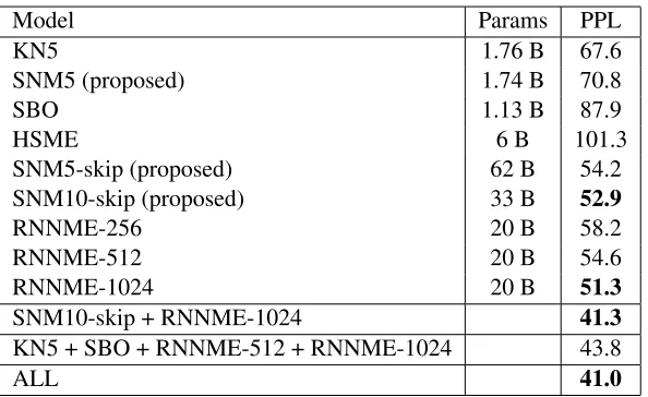
Describing these models however is beyond the scope of this paper. Instead we refer the reader to Chelba et al. (2014) for a detailed description. The table also lists the number of model parame-ters, which in the case of SNMLMs consist of the non-zero entries and precomputed row sums ofM.

When we compare the perplexity of SNM10-skip with the state-of-the-art RNNLM with 1024 hidden neurons (RNNME-1024), the difference is only 3%. Moreover, this small advantage comes at the cost of increased training and evaluation complexity. Inter-estingly, when we interpolate the two models, we have an additional gain of 20%, which shows that SNM10-skip and RNNME-1024 are also comple-mentary. As far as we know, the resulting perplex-ity of 41.3 is already the best ever reported on this corpus, beating the optimized combination of sev-eral models, reported in Chelba et al. (2014) by 6%. Finally, interpolation over all models shows that the contribution of other models as well as the additional perplexity reduction of 0.3 is negligible.

5.4 Runtime experiments

Model Params PPL

KN5 1.76 B 67.6

SNM5 (proposed) 1.74 B 70.8

SBO 1.13 B 87.9

HSME 6 B 101.3

SNM5-skip (proposed) 62 B 54.2

SNM10-skip (proposed) 33 B 52.9

RNNME-256 20 B 58.2

RNNME-512 20 B 54.6

RNNME-1024 20 B 51.3

SNM10-skip + RNNME-1024 41.3

KN5 + SBO + RNNME-512 + RNNME-1024 43.8

ALL 41.0

Table 3: Number of parameters and perplexity (PPL) results on the 1B Word Benchmark for the proposed models, compared to the models in Chelba et al. (2014).

More specifically, we compare the training runtime (in machine hours) of the best SNM model to the best RNN andn-gram models:

• KN5: 28 machine hours

• SNM5: 115 machine hours • SNM10-skip: 487 machine hours

• RNNME-1024: 5760 machine hours

As these models were trained using different archi-tectures (number of CPUs, type of distributed com-puting, etc.), a runtime comparison is inherently hard and we would therefore like to stress that these numbers should be taken with a grain of salt. How-ever, based on the order of magnitude we can clearly conclude that SNM’s reduced training complexity shown in Section 4 translates to a substantial reduc-tion in training time compared to RNNs. Moreover, the large difference between KN5 and SNM5 sug-gests that our vanilla implementation can be further improved to achieve even larger speed-ups.

6 Experiment 2: 44M Word Corpus

In addition to the experiments on the One Billion Word Benchmark, we also conducted experiments on a small subset of the LDC English Gigaword cor-pus. This has the advantage that the experiments are more easily reproducible and, since this corpus pre-serves the original sentence order, it also allows us to investigate SNM’s capabilities of modeling phe-nomena that cross sentence boundaries.

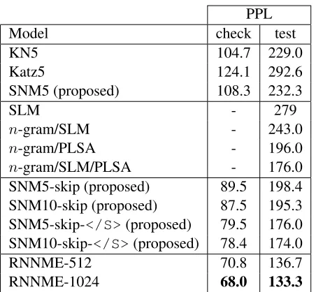
The corpus is the one used in Tan et al. (2012), which we acquired with the help of the authors and is now available at http://www.esat. kuleuven.be/psi/spraak/downloads/4. It consists of a training set of 44M tokens, a check set of 1.7M tokens and a test set of 13.7M tokens. The vocabulary contains 56k words which corresponds to an OOV rate of 0.89% and 1.98% for the check and test set, respectively. OOV words are mapped to an <UNK> token. The large difference in OOV rate between the check and test set is explained by the fact that the training data and check data are from the same source (Agence France-Presse), whereas the test data is drawn from CNA (Central News Agency of Taiwan) which seems to be out of domain relative to the training data. This discrepancy also shows in the perplexity results, presented in Table 4.

All of the described SNM models are initialized with meta-feature weights θk = 0 which are

up-dated using AdaGrad with accumulator ∆0 = 1

and scaling factorγ = 0.02over a single epoch of 10M training examples. The hash table for the meta-features was limited to 10M entries as increasing it yielded no significant improvements.

With regards ton-gram modeling, the results are

analogous to the 1B word experiment: SNM5 is close to KN5; both outperform Katz5 by a large

mar-4_{In order to comply with the LDC license, the data was}

gin. This is the case for the check set and the test set. Tan et al. (2012) showed that by crossing sen-tence boundaries, perplexities can be drastically re-duced. Although they did not publish any results on the check set, their mixture ofn-gram, syntac-tic language models and topic models achieved a perplexity of 176 on the test set, a 23% relative re-duction compared to KN5. A similar observation was made for the SNM models by adding a feature extractor (r, s, a) analogous to regular skip-grams, but withsnow denoting the number of skipped sen-tence boundaries </S> instead of words. Adding skip-</S> features with r +a = 4, 1 _≤ r _≤ 2 and1_≤s_≤10, yielded an even larger reduction of 26% than the one reported by Tan et al. (2012). On the check set we observed a 25% reduction.

The RNNME results are achieved with a setup similar to the one in Chelba et al. (2014). The main differences are related to the ME features (3-grams only instead of 10-grams and bag-of-words features) and the number of iterations over the training data (20 epochs instead of 10). These choices are related to the size of the training data. It can be seen from Table 4 that the best RNNME model outperforms the best SNM model by 13% on the check set. The out-of-domain test set shows that due to its compactness, RNNME is better suited for LM adaptation.

7 Conclusions and Future Work

We have presented SNM, a novel probability esti-mation technique for language modeling that can ef-ficiently incorporate arbitrary features. A first set of empirical evaluations on two data sets shows that SNM n-gram LMs perform almost as well as the well-established KN models. When we add skip-gram features, the models are able to match the state-of-the-art RNNLMs on the One Billion Word Benchmark (Chelba et al., 2014). Combining the two modeling techniques yields the best known re-sult on the benchmark which shows that the two models are complementary.

On a smaller subset of the LDC English Gigaword corpus, SNMLMs are able to exploit cross-sentence dependencies and outperform a mixture ofn-gram models, syntactic language models and topic mod-els. Although RNNLMs still outperform SNM by 13% on this corpus, a complexity analysis and

mea-PPL

Model check test

KN5 104.7 229.0

Katz5 124.1 292.6

SNM5 (proposed) 108.3 232.3

SLM - 279

n-gram/SLM - 243.0

n-gram/PLSA - 196.0

n-gram/SLM/PLSA - 176.0

SNM5-skip (proposed) 89.5 198.4

SNM10-skip (proposed) 87.5 195.3

SNM5-skip-</S>(proposed) 79.5 176.0 SNM10-skip-</S>(proposed) 78.4 174.0

RNNME-512 70.8 136.7

RNNME-1024 68.0 133.3

Table 4: Perplexity (PPL) results on the 44M corpus. On the small check set, SNM outperforms a mixture ofn -gram, syntactic language models (SLM) and topic models (PLSA), but RNNME performs best. The out-of-domain test set shows that due to its compactness, RNNME is better suited for LM adaptation.

sured runtimes show that the RNN comes at an in-creased training and evaluation time.

We conclude that the computational advantages of SNMLMs over both Maximum Entropy and RNN estimation promise an approach that has large flexi-bility in combining arbitrary features effectively and yet scales gracefully to large amounts of data.

Future work includes exploring richer features similar to Goodman (2001a), as well as richer meta-features in the adjustment model. A comparison of SNM models with Maximum Entropy at feature par-ity is also planned. One additional idea was pointed out to us by action editor Jason Eisner. Rather than using one-hot target vectors which emphasizes fit, it is possible to use low-dimensional word embed-dings. This would most likely yield a smaller model with improved generalization.

8 Acknowledgments

Appendix A Meta-feature Extraction Pseudocode

// Meta-features are represented as tuples (hash value, weight). // New meta-features are either added (metafeatures.Add(mf new)) or // joint (metafeatures.Join(mf new)) with the existing meta-features. // Strings are fingerprinted, counts are hashed.

functionCOMPUTE METAFEATURES(FeatureTargetPair pair)

// feature-related meta-features metafeatures ={}

metafeatures.Add(Fingerprint(pair.feature identity), 1.0) metafeatures.Add(Fingerprint(pair.feature type), 1.0) log count = log(pair.feature count) / log(2)

bucket1 = floor(log count) bucket2 = ceil(log count) weight1 = bucket2 - log count weight2 = log count - bucket1

metafeatures.Add(Hash(bucket1), weight1) metafeatures.Add(Hash(bucket2), weight2)

// target-related meta-features

metafeatures.Join(Fingerprint(pair.target identity), 1.0)

// feature-target-related meta-features

log count = log(pair.feature target count) / log(2) bucket1 = floor(log count)

bucket2 = ceil(log count) weight1 = bucket2 - log count weight2 = log count - bucket1

metafeatures.Join(Hash(bucket1), weight1) metafeatures.Join(Hash(bucket2), weight2)

return metafeatures

Appendix B Multinomial Gradient

∂logPmulti(y|x) ∂A(f, t) =

∂log(xTM)wk

∂Mf t −

∂logP_t0_∈V(xTM)t0

∂Mf t

∂Mf t ∂Af t

=

1 (xT_M)

wk

∂(xT_M) wk

∂Mf t −

1

P

t0_∈V(xTM)t0

∂P_t0_∈V(xTM)t0

∂Mf t

Mf t

=

xfyt

ˆ

ywk

− P xf

t0_∈V(xTM)t0

Mf t

=xfMf t

yt

ˆ

ywk

− P 1

t0_∈Vyˆt0

Appendix C Poisson Gradient

∂logPPois(y|x) ∂A(f, t) =

_∂P

t0_∈Vyt0log(xTM)t0

∂Mf t −

∂P_t0_∈V(xTM)t0

∂Mf t

∂Mf t ∂A(f, t)

=

1 (xT_M)

wk

∂(xT_M) wk

∂Mf t − xf

Mf t

=xfMf t

yt

ˆ

yw_k −1

Appendix D Distributing Negative Updates Over the entire training set, adding Cf∗

Cf tMf tonce on the targettthat occurs with featuref amounts to the

same as traversing all targetst0that co-occur withfin the training set and adding the termMf tto each:

Mf t

X

(f,t0_)∈T

xf = Cf∗

Cf t

Mf tCf t= Cf∗

Cf t Mf t

X

(f,t0_)∈T

xfyt0

Applying this to the second term of the Poisson gradient, we get:

∂logPPois(y|x)

∂A(f, t) =xfMf t

yt

ˆ

ywk

−xfMf t =xfMf t yt

ˆ

ywk

−xfytMf t Cf∗

Cf t

=xfytMf t

1 ˆ

ywk

−C_Cf∗ f t

Appendix E Leave-one-out Training

In leave-one-out training we exclude the event that generates the gradients from the counts used to compute those gradients. More specifically, for each training example(f, t)we let:

Cf∗ ←Cf∗−1 ifxf = 1

Cf t←Cf t−1 ifxf = 1, yt= 1

which means that the gradients for the positive and the negative examples are changed in a different way. Since Eq. (16) expresses the general update rule for both type of examples, we first have to separate it into updates for negative and positive examples and then adapt accordingly.

In particular, the second term of Eq. (16), i.e.−xfytMf tC_Cf_{f t}∗ is a distribution ofCf∗−Cf tnegative and Cf tpositive updates overCf tpositive examples:

−xfytMf t Cf∗

Cf t

=−xfytMf t

Cf∗−Cf t Cf t

+Cf t

Cf t

=−xfytMf t

Cf∗−Cf t Cf t −

xfytMf t

Furthermore, recall that the first term of Eq. (16), i.e. xfytMf t

ˆ

y_wk is non-zero only for positive examples, so

it can be added to the positive updates. We can then apply leave-one-out to positive and negative updates separately, ending up with:

∂logPPois(y|x)

∂A(f, t) =xfyt

( 1

ˆ

y+wk

−1)M_{f t}+−Cf∗−Cf t Cf t

M_{f t}−

whereM_{f t}−,M_{f t}+andyˆ+

wk are defined as follows:

M_{f t}− =eA(f,t,Cf∗−1,Cf t) Cf t

Cf∗−1

M_{f t}+ =eA(f,t,Cf∗−1,Cf t−1)Cf t−1

Cf∗−1 ˆ

References

Jerome Bellegarda. 2000. Exploiting Latent Semantic Information in Statistical Language Modeling. Pro-ceedings of the IEEE, 88(8), 1279–1296.

Yoshua Bengio, R´ejean Ducharme, Pascal Vincent, and Christian Janvin. 2003. A Neural Probabilistic Lan-guage Model.Journal of Machine Learning Research, 3, 1137–1155.

Thorsten Brants, Ashok C. Popat, Peng Xu, Franz J. Och, and Jeffrey Dean. 2007. Large Language Models in Machine Translation. Proceedings of EMNLP, 858– 867.

Ciprian Chelba and Frederick Jelinek. 2000. Struc-tured Language Modeling. Computer Speech and Lan-guage, 14(4), 283–332.

Ciprian Chelba, Tom´aˇs Mikolov, Mike Schuster, Qi Ge, Thorsten Brants, Phillipp Koehn, and Tony Robinson. 2014. One Billion Word Benchmark for Measuring Progress in Statistical Language Modeling. Proceed-ings of Interspeech, 2635–2639.

Ciprian Chelba and Fernando Pereira. 2016. Multi-nomial Loss on Held-out Data for the Sparse Non-negative Matrix Language Model. arXiv:1511.01574 [cs.CL].

Stanley F. Chen, Kristie Seymore, and Ronald Rosenfeld. 1998. Topic Adaptation for Language Modeling Us-ing Unnormalized Exponential Models. Proceedings

of ICASSP, 681–684.

Xie Chen, Xunying Liu, Mark Gales and Phil Woodland. 2015. Recurrent Neural Network Language Model Training with Noise Contrastive Estimation for Speech Recognition.Proceedings of ICASSP, 5411–5415. John Duchi, Elad Hazan and Yoram Singer. 2011.

Adap-tive Subgradient Methods for Online Learning and Stochastic Optimization. Journal of Machine Learn-ing Research, 12, 2121–2159.

Jeffrey L. Elman. 1990. Finding Structure in Time. Cog-nitive Science, 14(2), 179–211.

Ahmad Emami. 2006. A Neural Syntactic Language Model.Ph.D. Thesis, Johns Hopkins University. Joshua T. Goodman. 2001a. A Bit of Progress in

Lan-guage Modeling, Extended Version. Technical Report

MSR-TR-2001-72.

Joshua T. Goodman. 2001b. Classes for Fast Maximum Entropy Training. Proceedings of ICASSP, 561–564. Michael Gutmann and Aapo Hyv¨arinen. 2012.

Noise-contrastive Estimation of Unnormalized Statistical Models, with Applications to Natural Image Statistics.

Journal of Machine Learning Research, 13(1), 307–

361.

Xuedong Huang, Fileno Alleva, Mei-Yuh Hwang, and Ronald Rosenfeld. 1993. An Overview of the

SPHINX-II Speech Recognition System. Computer

Speech and Language, 2, 137–148.

Slava M. Katz. 1987. Estimation of Probabilities from Sparse Data for the Language Model Component of a Speech Recognizer. IEEE Transactions on Acoustics, Speech and Signal Processing, 35(3), 400–401. Dietrich Klakow. 1998. Log-linear Interpolation of

Lan-guage Models. Proceedings of ICSLP, 1695–1698. Reinhard Kneser and Hermann Ney. 1995. Improved

Backing-Off for M-Gram Language Modeling.

Pro-ceedings of ICASSP, 181–184.

John Langford, Lihong Li and Alex Strehl. 2007. Vowpal Wabbit Online Learning Project. http:// hunch.net/?p=309.

Kuzman Ganchev and Mark Dredze. 2008. Small Statis-tical Models by Random Feature Mixing. Proceedings of the ACL-2008 Workshop on Mobile Language Pro-cessing, 19–20.

Hai-Son Le, Ilya Oparin, Alexandre Allauzen, Jean-Luc Gauvain and Franc¸ois Yvon. 2013. Structured Output Layer Neural Network Language Models for Speech Recognition. IEEE Transactions on Audio, Speech &

Language Processing, 21, 195–204.

Su-in Lee, Vassil Chatalbashev, David Vickrey and Daphne Koller. 2007 Learning a Meta-level Prior for Feature Relevance from Multiple Related Tasks.

Pro-ceedings of ICML, 489–496.

Tom´aˇs Mikolov, Anoop Deoras, Daniel Povey, Luk´as Burget and Jan Cernock´y. 2011. Strategies for Train-ing Large Scale Neural Network Language Models.

Proceedings of ASRU, 196–201.

Tom´aˇs Mikolov. 2012. Statistical Language Models Based on Neural Networks. Ph.D. Thesis, Brno Uni-versity of Technology.

Frederic Morin and Yoshua Bengio. 2005. Hierarchical Probabilistic Neural Network Language Model.

Pro-ceedings of AISTATS, 246–252.

Hermann Ney, Ute Essen, and Reinhard Kneser. 1994. On Structuring Probabilistic Dependences in Stochas-tic Language Modeling. Computer Speech and Lan-guage, 8, 1–38.

Rene Pickhardt, Thomas Gottron, Martin K¨orner, Paul G. Wagner, Till Speicher, and Steffen Staab. 2014. A Generalized Language Model as the Combination of Skipped n-grams and Modified Kneser-Ney

Smooth-ing.Proceedings of ACL, 1145–1154.

Ronald Rosenfeld. 1994. Adaptive Statistical Language Modeling: A Maximum Entropy Approach. Ph.D. Thesis, Carnegie Mellon University.

Ronald Rosenfeld, Stanley F. Chen, and Xiaojin Zhu. 2001. Whole-sentence Exponential Language Mod-els: a Vehicle for Linguistic-Statistical Integration.

Holger Schwenk and Jean-Luc Gauvain. 2004. Neural Network Language Models for Conversational Speech Recognition.Proceedings of ICSLP, 1215-1218. Holger Schwenk and Jean-Luc Gauvain. 2005.

Train-ing Neural Network Language Models On Very Large Corpora.Proceedings of EMNLP, 201–208.

Holger Schwenk. 2007. Continuous Space Language Models. Computer Speech and Language, 21, 492– 518.

Mittul Singh and Dietrich Klakow. 2013. Comparing RNNs and Log-linear Interpolation of Improved Skip-model on Four Babel Languages: Cantonese, Pashto, Tagalog, Turkish. Proceedings of ICASSP, 8416– 8420.

Martin Sundermeyer, Ralf Schl¨uter, and Hermann Ney. 2012. LSTM Neural Networks for Language Model-ing.Proceedings of Interspeech, 194–197.

Ming Tan, Wenli Zhou, Lei Zheng and Shaojun Wang. 2012. A Scalable Distributed Syntactic, Semantic, and Lexical Language Model. Computational Linguistics, 38(3), 631–671.

Puyang Xu, Asela Gunawardana, and Sanjeev Khudan-pur. 2011. Efficient Subsampling for Training Com-plex Language Models. Proceedings of EMNLP, 1128–1136.