SECTOR: A Neural Model for Coherent Topic
Segmentation and Classification
Sebastian Arnold Rudolf Schneider Beuth University of Applied
Sciences Berlin, Germany {sarnold, ruschneider}@
beuth-hochschule.de
Philippe Cudr´e-Mauroux University of Fribourg
Fribourg, Switzerland
Felix A. Gers Alexander L¨oser Beuth University of Applied
Sciences Berlin, Germany {gers, aloeser}@
beuth-hochschule.de
Abstract
When searching for information, a human reader first glances over a document, spots relevant sections, and then focuses on a few sentences for resolving her intention. How-ever, the high variance of document structure complicates the identification of the salient topic of a given section at a glance. To tackle this challenge, we present SECTOR, a model to support machine reading systems by segmenting documents into coherent sections and assigning topic labels to each section. Our deep neural network architecture learns a latent topic embedding over the course of a document. This can be leveraged to classify local topics from plain text and segment a document at topic shifts. In addition, we contribute WikiSection, a publicly available data set with 242k labeled sections in English and German from two distinct domains: dis-eases and cities. From our extensive evaluation of 20 architectures, we report a highest score of 71.6% F1 for the segmentation and classification of 30 topics from the English city domain, scored by our SECTOR long short-term memory model with Bloom filter embeddings and bidirectional segmentation. This is a significant improvement of 29.5 points F1 over state-of-the-art CNN classifiers with baseline segmentation.
1 Introduction
Today’s systems for natural language understand-ing are composed of buildunderstand-ing blocks that extract semantic information from the text, such as named entities, relations, topics, or discourse structure. In traditional natural language processing (NLP), these extractors are typically applied to bags of
words or full sentences (Hirschberg and Manning, 2015). Recent neural architectures build upon pre-trained word or sentence embeddings (Mikolov et al., 2013; Le and Mikolov, 2014), which focus on semantic relations that can be learned from large sets of paradigmatic examples, even from long ranges (Dieng et al., 2017).
From a human perspective, however, it is mostly the authors themselves who help best to understand a text. Especially in long documents, an author thoughtfully designs a readable structure and guides the reader through the text by arranging topics into coherent passages (Glavaˇs et al., 2016). In many cases, this structure is not formally ex-pressed as section headings (e.g., in news articles, reviews, discussion forums) or it is structured according to domain-specific aspects (e.g., health reports, research papers, insurance documents).
Ideally, systems for text analytics, such as topic detection and tracking (TDT) (Allan, 2002), text summarization (Huang et al., 2003), information retrieval (IR) (Dias et al., 2007), or question an-swering (QA) (Cohen et al., 2018), could access a document representation that is aware of both topical (i.e., latent semantic content) and struc-tural information (i.e., segmentation) in the text (MacAvaney et al., 2018). The challenge in building such a representation is to combine these two dimensions that are strongly interwoven in the author’s mind. It is therefore important to understand topic segmentation and classification as a mutual task that requires encoding both topic information and document structure coherently.
In this paper, we present SECTOR,1an end-to-end model that learns an embedding of latent topics
1Our source code is available under the Apache License
2.0 at https://github.com/sebastianarnold/ SECTOR.
169
from potentially ambiguous headings and can be applied to entire documents to predict local topics on sentence level. Our model encodes topical in-formation on a vertical dimension and structural information on a horizontal dimension. We show that the resulting embedding can be leveraged in a downstream pipeline to segment a document into coherent sections and classify the sections into one of up to 30 topic categories reaching 71.6%F1—or alternatively, attach up to 2.8k topic labels with 71.1% mean average precision (MAP). We further show that segmentation performance of our bidirectional long short-term memory (LSTM) architecture is comparable to specialized state-of-the-art segmentation methods on various real-world data sets.
To the best of our knowledge, the combined task of segmentation and classification has not been approached on the full document level before. There exist a large number of data sets for text segmentation, but most of them do not reflect real-world topic drifts (Choi, 2000; Sehikh et al., 2017), do not include topic labels (Eisenstein and Barzilay, 2008; Jeong and Titov, 2010; Glavaˇs et al., 2016), or are heavily normalized and too small to be used for training neural networks (Chen et al., 2009). We can utilize a generic segmentation data set derived from Wikipedia that includes headings (Koshorek et al., 2018), but there is also a need in IR and QA for supervised structural topic labels (Agarwal and Yu, 2009; MacAvaney et al., 2018), different languages and more specific domains, such as clinical or biomedical research (Tepper et al., 2012; Tsatsaronis et al., 2012), and news-based TDT (Kumaran and Allan, 2004; Leetaru and Schrodt, 2013).
Therefore we introduce WIKISECTION,2 a large novel data set of 38k articles from the English and German Wikipedia labeled with 242k sec-tions, original headings, and normalized topic labels for up to 30 topics from two domains: dis-easesandcities. We chose these subsets to cover both clinical/biomedical aspects (e.g., symptoms, treatments, complications) and news-based topics (e.g., history, politics, economy, climate). Both article types are reasonably well-structured ac-cording to Wikipedia guidelines (Piccardi et al., 2018), but we show that they are also
comple-2The data set is available under the CC BY-SA 3.0
license at https://github.com/sebastianarnold/ WikiSection.
mentary: Diseases is a typical scientific domain with low entropy (i.e., very narrow topics, precise language, and low word ambiguity). In contrast, cities resembles a diversified domain, with high entropy (i.e., broader topics, common language, and higher word ambiguity) and will be more applicable to for example, news, risk reports, or travel reviews.
We compare SECTOR to existing segmenta-tion and classificasegmenta-tion methods based on latent Dirichlet allocation (LDA), paragraph embed-dings, convolutional neural networks (CNNs), and recurrent neural networks (RNNs). We show that SECTOR significantly improves these methods in a combined task by up to 29.5 points F1 when applied to plain text with no given segmentation.
The rest of this paper is structured as follows: We introduce related work in Section 2. Next, we describe the task and data set creation process in Section 3. We formalize our model in Section 4. We report results and insights from the evaluation in Section 5. Finally, we conclude in Section 6.
2 Related Work
The analysis of emerging topics over the course of a document is related to a large number of research areas. In particular, topic modeling (Blei et al., 2003) and TDT (Jin et al., 1999) focus on representing and extracting the semantic topical con-tent of text. Text segmentation (Beeferman et al. 1999) is used to split documents into smaller co-herent chunks. Finally, text classification (Joachims 1998) is often applied to detect topics on text chunks. Our method unifies those strongly inter-woven tasks and is the first to evaluate the com-bined topic segmentation and classification task using a corresponding data set with long structured documents.
closely related domain keyphrases. Yeh et al. (2016) proposed a conceptual dynamic LDA model for tracking topics in conversations. Bhatia et al. (2016) utilized Wikipedia document titles to learn neural topic embeddings and assign doc-ument labels. Dieng et al. (2017) focused on the issue of long-range dependencies and proposed a latent topic model based on RNNs. However, the authors did not apply the RNN to predict local topics.
Text segmentation has been approached with a wide variety of methods. Early unsuper-vised methods utilized lexical overlap statistics (Hearst 1997; Choi 2000), dynamic programming (Utiyama and Isahara, 2001), Bayesian models (Eisenstein and Barzilay, 2008), or pointwise boundary sampling (Du et al., 2013) on raw terms. Later, supervised methods included topic mod-els (Riedl and Biemann, 2012) by calculating a coherence score using dense topic vectors ob-tained by LDA. Bayomi et al. (2015) exploited ontologies to measure semantic similarity be-tween text blocks. Alemi and Ginsparg (2015) and Naili et al. (2017) studied how word embeddings can improve classical segmentation approaches. Glavaˇs et al. (2016) utilized semantic relatedness of word embeddings by identifying cliques in a graph.
More recently, Sehikh et al. (2017) utilized LSTM networks and showed that cohesion be-tween bidirectional layers can be leveraged to predict topic changes. In contrast to our method, the authors focused on segmenting speech recog-nition transcripts on word level without explicit topic labels. The network was trained with super-vised pairs of contrary examples and was mainly evaluated on artificially segmented documents. Our approach extends this idea so it can be applied to dense topic embeddings which are learned from raw section headings.
Wang et al. (2017) tackled segmentation by training a CNN to learn coherence scores for text pairs. Similar to Sehikh et al. (2017), the network was trained with short contrary examples and no topic objective. The authors showed that their pointwise ranking model performs well on data sets by Jeong and Titov (2010). In contrast to our method, the ranking algorithm strictly requires a given ground truth number of segments for each document and no topic labels are predicted.
Koshorek et al. (2018) presented a large new data set for text segmentation based on Wikipedia
that includes section headings. The authors intro-duced a neural architecture for segmentation that is based on sentence embeddings and four layers of bidirectional LSTM. Similar to Sehikh et al. (2017), the authors used a binary segmentation objective on the sentence level, but trained on entire documents. Our work takes up this idea of end-to-end training and enriches the neural model with a layer of latent topic embeddings that can be utilized for topic classification.
Text classification is mostly applied at the paragraph or sentence level using machine learning methods such as support vector machines (Joachims, 1998) or, more recently, shallow and deep neural networks (Le et al., 2018; Conneau et al., 2017). Notably, paragraph vectors (Le and Mikolov, 2014) is an extension of word2vec for learning fixed-length distributed representations from texts of arbitrary length. The resulting model can be utilized for classification by providing paragraph labels during training. Furthermore, Kim (2014) has shown that CNNs combined with pre-trained task-specific word embeddings achieve the highest scores for various text classification tasks.
Combined approachesof topic segmentation and classification are rare to find. Agarwal and Yu (2009) classified sections of BioMed Central articles into four structural classes (introduction, methods, results, and discussion). However, their manually labeled data set only contains a sample of sentences from the documents, so they evaluated sentence classification as an isolated task. Chen et al. (2009) introduced two Wikipedia-based data sets for segmentation, one about large cities, the second about chemical elements. Although these data sets have been used to evaluate word-level and sentence-level segmentation (Koshorek et al., 2018), we are not aware of any topic classification approach on this data set.
(1) Plain Text
without headings (1) Plain Text
without headings (2) Topic Distributionover sequence (2) Topic Distribution
over sequence Segmentation(3) Topic
(3) Topic Segmentation
disease.diagnosis disease.cause disease.symptom
(4) Topic Classification
[image:4.595.71.528.56.208.2](4) Topic Classification
Figure 1: Overview of the WIKISECTIONtask: (1) The input is a plain text documentDwithout structure information. (2) We assume the sentencess1...N contain a coherent sequence of local topicse1...N. (3) The task is to segment
the document into coherent sectionsS1...M and (4) to classify each section with a topic labely1...M.
Eventually, we were inspired by passage re-trieval (Liu and Croft, 2002) as an important downstream task for topic segmentation and clas-sification. For example, Hewlett et al. (2016) pro-posed WikiReading, a QA task to retrieve values from sections of long documents. The objective of TREC Complex Answer Retrieval is to retrieve a ranking of relevant passages for a given outline of hierarchical sections (Nanni et al., 2017). Both tasks highly depend on a building block for local topic embeddings such as our proposed model.
3 Task Overview and Data set
We start with a definition of the WIKISECTION machine reading task shown in Figure 1. We take a document D = hS,Ti consisting of N
consecutive sentences S = [s1, . . . ,sN] and
empty segmentation T = ∅ as input. In our
example, this is the plain text of a Wikipedia article (e.g., aboutTrichomoniasis3) without any section information. For each sentence sk,
we assume a distribution of local topics ek
that gradually changes over the course of the document.
The task is to split D into a sequence of distinct topic sectionsT= [T1, . . . ,TM], so that
each predicted section Tj = hSj,yji contains
a sequence of coherent sentences Sj ⊆ S and
a topic label yj that describes the common
topic in these sentences. For the document
3https://en.wikipedia.org/w/index.php?
title=Trichomoniasis&oldid=814235024.
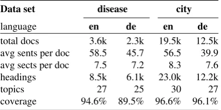
Data set disease city
language en de en de
total docs 3.6k 2.3k 19.5k 12.5k avg sents per doc 58.5 45.7 56.5 39.9 avg sects per doc 7.5 7.2 8.3 7.6
headings 8.5k 6.1k 23.0k 12.2k
topics 27 25 30 27
coverage 94.6% 89.5% 96.6% 96.1%
Table 1: Data set characteristics fordisease(German:
Krankheit) andcity(German:Stadt).Headingsdenotes the number of distinct section and subsection headings among the documents.Topicsstands for the number of topic labels after synset clustering.Coveragedenotes the proportion of headings covered by topics; the remaining headings are labeled asother.
Trichomoniasis, the sequence of topic labels
is y1...M = [ symptom, cause, diagnosis,
prevention,treatment,complication,
epidemiology].
3.1 WikiSection Data Set
For the evaluation of this task, we created WIKI-SECTION, a novel data set containing a gold stan-dard of 38k full-text documents from English and German Wikipedia comprehensively annotated with sections and topic labels (see Table 1).
The documents originate from recent dumps in English4and German.5We filtered the collection
4https://dumps.wikimedia.org/enwiki/
20180101.
5https://dumps.wikimedia.org/dewiki/
[image:4.595.307.527.286.395.2]using SPARQL queries against Wikidata (Tanon et al., 2016). We retrieved instances of Wikidata categoriesdisease(Q12136) and their subcategories (e.g., Trichomoniasis or Pertussis) or city(Q515) (e.g.,LondonorMadrid).
Our data set contains the article abstracts, plain text of the body, positions of all sections given by the Wikipedia editors with their original head-ings (e.g., "Causes | Genetic sequence") and a normalized topic label (e.g., disease.
cause). We randomized the order of documents
and split them into 70% training, 10% validation, 20% test sets.
3.2 Preprocessing
To obtain plain document text, we used Wiki-extractor,6split the abstract sections and stripped all section headings and other structure tags except newline characters and lists.
Vocabulary Mismatch in Section Headings. Table 2 shows examples of section headings from disease articles separated into head (most common), torso (frequently used), and tail (rare). Initially, we expected articles to share congruent structure in naming and order. Instead, we observe a high variance with 8.5k distinct headings in the diseases domain and over 23k for English cities. A closer inspection reveals that Wikipedia authors utilize headings at different granularity levels, frequently copy and paste from other articles, but also introduce synonyms or hyponyms, which leads to avocabulary mismatch problem(Furnas et al., 1987). As a result, the distribution of head-ings is heavy-tailed across all articles. Roughly 1% of headings appear more than 25 times whereas the vast majority (88%) appear 1 or 2 times only.
3.3 Synset Clustering
In order to use Wikipedia headlines as a source for topic labels, we contribute a normalization method to reduce the high variance of headings to a few representative labels based on the clustering of BabelNet synsets (Navigli and Ponzetto, 2012). We create a set H that contains all headings in the data set and use the BabelNet API to match7 each headingh ∈ H to its corresponding
6http://attardi.github.io/wikiextractor/. 7We match lemmas of main senses and compounds to
synsets of type NOUN CONCEPT.
rank headingh labely H freq
0 Diagnosis diagnosis 0.68 3,854 1 Treatment treatment 0.69 3,501 2 Signs and
Symptoms
symptom 0.68 2,452
. . . 21 Differential
Diagnosis
diagnosis 0.23 236
22 Pathogenesis mechanism 0.16 205 23 Medications medication 0.14 186
. . . 8,494 Usher Syndrome
Type IV
classification 0.00 1
8,495 False Melanose Lesions
other 0.00 1
8,496 Cognitive Therapy
[image:5.595.307.526.58.277.2]treatment 0.00 1
Table 2: Frequency and entropy (H) of top-3 head and randomly selected torso and tail headings for category diseases in the English Wikipedia.
synsets Sh ⊂ S. For example, "Cognitive
behavioral therapy"is assigned to synset
bn:03387773n. Next, we insert all matched
synsets into an undirected graph G with nodes
s ∈ S and edges e. We create edges between all synsets that match among each other with a lemma h0 ∈ H. Finally, we apply a community detection algorithm (Newman, 2006) onGto find dense clusters of synsets. We use these clusters as normalized topics and assign the sense with most outgoing edges as representative label, in our example e.g.therapy.
From this normalization step we obtain 598 synsets that we prune using the head/tail divi-sion rulecount(s)< |S1|P
si∈Scount(si)(Jiang,
2012). This method covers over 94.6% of all headings and yields 26 normalized labels and one
otherclass in the English disease data set. Table 1 shows the corresponding numbers for the other data sets. We verify our normalization process by man-ual inspection of 400 randomly chosen heading– label assignments by two independent judges and report an accuracy of 97.2% with an average observed inter-annotator agreement of 96.0%.
4 SECTOR Model
topic vectors
Wikipedia Articles
Raw Text
BabelNet
training targets
training targets
Prepro-cessing
Prepro-cessing
Synset Clustering
Synset Clustering
(1) Sentence Encoding (1) Sentence
Encoding (2) Topic EmbeddingBLSTM (2) Topic Embedding
BLSTM
(3a) Topic Classification
single-label (3a) Topic Classification
single-label
(4) Topic Segmentation
sentence-level (4) Topic Segmentation
sentence-level
(A) WikiSection Training and Evaluation Data (B) SECTOR Model Inference
(3b) Heading Classification multi-label (3b) Heading Classification multi-label Headings
~1.5k words
Topic Labels
~25 classes
Headings Task
multi-labeled sections
Topics Task
[image:6.595.71.528.56.204.2]single-labeled sections
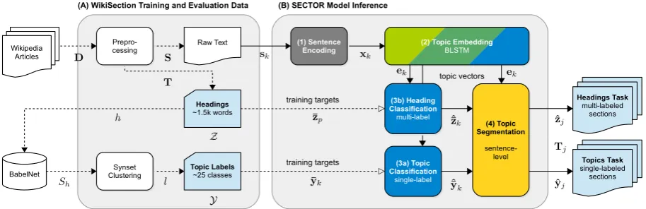
Figure 2: Training and inference phase of segmentation and topic classification (SECTOR). For training (A), we preprocess Wikipedia documents to supply a ground truth for segmentationT, headingsZ and topic labelsY. During inference (B), we invoke SECTORwith unseen plain text to predict topic embeddingsekon sentence level.
The embeddings are used to segment the document and classify headingsˆzjand normalized topic labelsˆyj.
described in Section 3, we aim to detectMsections
T1...M in a document Dand assign topic labels
yj = topic(Sj), where j = 1, . . . , M. Because
we do not know the expected number of sections, we formulate the objective of our model on the sentence level and later segment based on the predictions. Therefore, we assign each sentence
sk a sentence topic label¯yk = topic(sk), where
k = 1, . . . , N. Thus, we aim to predict coherent
sections with respect to document context:
p(y¯1, ... ,¯yN |D) = N
Y
k=1
p(¯yk|s1, ... ,sN) (1)
We approach two variations of this task: For WIKISECTION-topics, we choose a single topic label yj ∈ Y out of a small number of
nor-malized topic labels. However, from this sim-plified classification task arises an entailment problem, because topics might be hierarchically structured. For example, a section with
head-ing"Treatment | Gene Therapy" might
describe genetics as a subtopic of treat-ment. Therefore, we also approach an extended task WIKISECTION-headings to capture ambiguity in a heading, We follow the CBOW approach (Mikolov et al., 2013) and assign all words in the heading zj ⊂ Z as multi-label bag over
the original heading vocabulary. This turns our problem into a ranked retrieval task with a large number of ambiguous labels, similar to Prabhu and Varma (2014). It further eliminates the need for normalized topic labels. For both tasks, we aim to maximize the log likelihood
of model parameters Θ on section and sentence level:
L(Θ) =
M
X
j=1
logp(yj |s1, ... ,sN; Θ)
¯ L(Θ) =
N
X
k=1
logp(¯yk|s1, ... ,sN; Θ)
(2)
Our SECTORarchitecture consists of four stages, shown in Figure 2: sentence encoding, topic embedding, topic classification and topic segmen-tation. We now discuss each stage in more detail.
4.1 Sentence Encoding
The first stage of our SECTOR model transforms each sentenceskfrom plain text into a fixed-size
sentence vector xk that serves as input into the
neural network layers. Following Hill et al. (2016), word order is not critical for document-centric evaluation settings such as our WIKISECTIONtask. Therefore, we mainly focus on unsupervised compositional sentence representations.
Bag-of-Words Encoding. As a baseline, we compose sentence vectors using a weighted bag-of-words scheme. Let I(w) ∈ {0,1}|V| be the
indicator vector, such that I(w)(i) = 1 iff w is
the i-th word in the fixed vocabulary V, and let tf-idf(w) be the TF-IDF weight of w in the corpus. We define the sparse bag-of-words encodingxbow∈R|V|as follows:
xbow(s) = X
w∈s
Bloom Filter Embedding. For largeVand long documents, input matrices grow too large to fit into GPU memory, especially with larger batch sizes. Therefore we apply a compression technique for sparse sentence vectors based on Bloom filters (Serr`a and Karatzoglou, 2017). A Bloom filter projects every item of a set onto a bit array A(i) ∈ {0,1}m using k independent hash
functions. We use the sum of bit arrays per word as compressed Bloom embeddingxbloom ∈Nm:
xbloom(s) = X
w∈s
k
X
i=1
A hashi(w)
(4)
We set parameters to m = 4096 and k = 5 to achieve a compression factor of 0.2, which showed good performance in the original paper.
Sentence Embeddings. We use the strategy of Arora et al. (2017) to generate a distribu-tional sentence representation based on pre-trained word2vec embeddings (Mikolov et al., 2013). This method composes a sentence vectorvemb∈Rdfor all sentences using a probability-weighted sum of word embeddings vw ∈ Rd with α = 10−4,
and subtracts the first principal component u of the embedding matrix[vs:s∈S]:
vs =
1 |S|
X
w∈s
α
α+p(w) vw
xemb(s) =vs−uuTvs
(5)
4.2 Topic Embedding
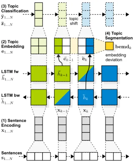
[image:7.595.306.525.54.320.2]We model the second stage in our architecture to produce a dense distributional representation of latent topics for each sentence in the document. We use two layers of LSTM (Hochreiter and Schmidhuber, 1997) with forget gates (Gers et al., 2000) connected to read the document in the forward and backward direction (Graves, 2012). We feed the LSTM outputs to a ‘‘bottleneck’’ layer with tanh activation as topic embedding. Figure 3 shows these layers in context of the complete architecture. We can see that context from left (k − 1) and right (k + 1) affects forward and backward layers independently. It is therefore important to separate these weights in the embedding layer to precisely capture the difference between sentences at section boundaries. We modify our objective given in Equation (2) accordingly with long-range
depen-(4) Topic Segmentation
(1) Sentence Encoding (2) Topic Embedding (3) Topic Classification
LSTM fw
Sentences LSTM bw
topic shift
[image:7.595.105.295.441.486.2]embedding deviation
Figure 3: Neural network architecture SECTOR. The recurrent model consists of stacked LSTM, embedding and output layers that are optimized on document level and later accessed during inference in stages 1–4.
dencies from forward and backward layers of the LSTM:
L(Θ) =
N
X
k=1
logp(¯yk|x1...k−1;Θ~,Θ0)
+ logp(¯yk|xk+1...N;Θ~ ,Θ0)
(6)
Note that we separate network parameters Θ~ andΘ~ for forward and backward directions of the LSTM, and tie the remaining parameters Θ0 for the embedding and output layers. This strategy couples the optimization of both directions into the same vector space without the need for an additional loss function. The embeddings e1...N
are calculated from the context-adjusted hidden statesh0k of the LSTM cells (here simplified as fLSTM) through the bottleneck layer:
~hk =fLSTM(xk, ~h0k−1, ~Θ)
~h
k =fLSTM(xk, 0~hk+1, ~Θ)
~ek = tanh(Weh~hk+be)
~
ek = tanh(Weh k~h +be)
(7)
Now, a simple concatenation of the embeddings
ek = ~ek⊕ek~ can be used as topic vector by
4.3 Topic Classification
The third stage in our architecture is the output layer that decodes the class labels. To learn model parametersΘrequired by the embedding, we need to optimize the full model for a training target. For the WIKISECTION-topics task, we use a simple one-hot encoding ¯y ∈ {0,1}|Y| of the topic labels constructed in Section 3.3 with a softmax activation output layer. For the WIKISECTION-headings task, we encode each heading as lower-case bag-of-words vector¯z∈ {0,1}|Z|, such that
¯z(i) = 1 iff the i-th word in Z is contained in the heading, for example,¯zk=ˆ{gene,therapy,
treatment}. We then use a sigmoid activation
function:
ˆ ¯
yk = softmax(Wye~ek+Wyeek~ +by)
ˆ
¯zk = sigmoid(Wze~ek+Wzeek~ +bz)
(8)
Ranking Loss for Multi-Label Optimization. The multi-label objective is to maximize the like-lihood of every word that appears in a heading:
L(Θ) =
N
X
k=1 |Z| X
i=1
logp(¯z(ki) |x1...N; Θ) (9)
For training this model, we use a variation of the logistic pairwise ranking loss function proposed by dos Santos et al. (2015). It learns to maximize the distance between positive and negative labels:
L= log 1 + exp(γ(m+−score+(x))) + log 1 + exp(γ(m−+ score−(x))) (10)
We calculate the positive term of the loss by taking all scores of correct labelsy+into account. We average over all correct scores to avoid a too-strong positive push on the energy surface of the loss function (LeCun et al., 2006). For the negative term, we only take the most offending example
y−among all incorrect class labels.
score+(x) = 1 |y+|
X
y∈y+
sθ(x)(y)
score−(x) = arg max
y∈y−
sθ(x)(y)
(11)
Here, sθ(x)(y) denotes the score of label y for
input x. We follow the authors and set scaling factorγ = 2, marginsm+= 2.5, andm− = 0.5.
4.4 Topic Segmentation
In the final stage, we leverage the information encoded in the topic embedding and output layers to segment the document and classify each section.
Baseline Segmentation Methods. As a simple baseline method, we use prior information from the text and split sections at newline characters (NL). Additionally, we merge two adjacent sec-tions if they are assigned the same topic label after classification. If there is no newline information available in the text, we use a maximum label (max) approach: We first split sections at every sentence break (i.e.,Sj =sk;j=k= 1, . . . , N)
and then merge all sections that share at least one label in the top-2 predictions.
Using Deviation of Topic Embeddings for Segmentation. All information required to clas-sify each sentence in a document is contained in our dense topic embedding matrix E =
[e1, . . . ,eN]. We are now interested in the
vec-tor space movement of this embedding over the sequence of sentences. Therefore, we apply a number of transformations adapted from Laplacian-of-Gaussian edge detection on images (Ziou and Tabbone, 1998) to obtain the magnitude of embedding deviation (emd) per sentence. First, we reduce the dimensionality of E to D
dimensions using PCA, that is, we solve E =
UΣWT using singular value decomposition and then project E on the D principal components
ED =EWD. Next, we apply Gaussian smoothing
to obtain a smoothed matrix ED0 by convolution with a Gaussian kernel with varianceσ2. From the reduced and smoothed embedding vectorse01...N
we construct a sequence of deviations d1...N by
calculating the stepwise difference using cosine distance:
dk = cos(e0k−1,e0k) =
e0k−1·e0k
ke0
k−1kke0kk
(12)
Finally we apply the sequence d1...N with
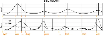
parameters D = 16 and σ = 2.5 to locate the spots of fastest movement (see Figure 4), i.e. all
kwhere dk−1 <dk > dk+1;k = 1. . . N in our discrete case. We use these positions to start a new section.
Figure 4: Embedding deviations emdk andbemdk
of the smoothed SECTORtopic embeddings for example document Trichomoniasis. The plot shows the first derivative of vector movement over sentences
k= 1, . . . Nfrom left to right. Predicted segmentation
is shown as black lines, the axis labels indicate ground truth segmentation.
embedding deviation (bemd) as geometric mean of the forward and backward difference:
d0k=
q cos(e~0
k−1, ~e0k)·cos(e0~ k, ~e0k+1) (13)
After segmentation, we assign each segment the mean class distribution of all contained sentences:
ˆ yj =
1 |Sj |
X
si∈Sj
ˆ ¯
yi (14)
Finally, we show in the evaluation that our SECTORmodel, which was optimized for sentences
¯
yk, can be applied to the WIKISECTION task to predict coherently labeled sectionsTj =hSj,yˆji.
5 Evaluation
We conduct three experiments to evaluate the segmentation and classification task introduced in Section 3. The WIKISECTION-topics experiment constitutes segmentation and classification of each section with a single topic label out of a small number of clean labels (25–30 topics). The WIKISECTION-headings experiment extends the classification task to multi-label per section with a larger target vocabulary (1.0k–2.8k words). This is important, because often there are no clean topic labels available for training or evaluation. Finally, we conduct a third experiment to see how SECTOR performs across existing segmentation data sets.
Evaluation Data Sets. For the first two exper-iments we use the WIKISECTION data sets intro-duced in Section 3.1, which contain documents about diseases and cities in both English and German. The subsections are retained with full granularity. For the third experiment, text seg-mentation results are often reported on artificial data sets (Choi, 2000). It was shown that this
scenario is hardly applicable to topic-based seg-mentation (Koshorek et al., 2018), so we restrict our evaluation to real-world data sets that are publicly available. The Wiki-727k data set by Koshorek et al. (2018) contains Wikipedia articles with a broad range of topics and their top-level sections. However, it is too large to compare exhaustively, so we use the smallerWiki-50subset. We further use theCitiesandElements data sets introduced by Chen et al. (2009), which also provide headings. These sets are typically used for word-level segmentation, so they don’t contain any punctuation and are lowercased. Finally, we use the Clinical Textbook chapters introduced by Eisenstein and Barzilay (2008), which do not supply headings.
Text Segmentation Models. We compare SEC -TOR to common text segmentation methods as baseline,C99(Choi, 2000) andTopicTiling(Riedl and Biemann, 2012) and the state-of-the-art TextSegsegmenter (Koshorek et al., 2018). In the third experiment we report numbers forBayesSeg (Eisenstein and Barzilay, 2008) (configured to predict with unknown number of segments) and GraphSeg(Glavaˇs et al., 2016).
Classification Models. We compare SECTORto existing models for single and multi-label sen-tence classification. Because we are not aware of any existing method for combined segmentation and classification, we first compare all methods using given prior segmentation from newlines in the text (NL) and then additionally apply our own segmentation strategies for plain text input: maximum label (max), embedding deviation (emd) and bidirectional embedding deviation (bemd).
headings (CNN>H). We configured the models using the hyperparameters given in the paper and trained the model using a batch size of 256 sentences for 20 epochs with learning rate 0.01.
SECTOR Configurations. We evaluate the
var-ious configurations of our model discussed in prior sections. SEC>T depicts the single-label topic classification model which uses a softmax activation output layer, SEC>H is the multi-label variant with a larger output and sigmoid activations. Other options are: bag-of-words sentence encoding (+bow), Bloom filter encoding (+bloom) and sentence embeddings (+emb); multi-class cross-entropy loss (as default) and ranking loss (+rank).
We have chosen network hyperparameters us-ing grid search on the en disease validation set and keep them fixed over all evaluation runs. For all configurations, we set LSTM layer size to 256, topic embeddings dimension to 128. Models are trained on the complete train splits with a batch size of 16 documents (reduced to 8 for bag-of-words), 0.01 learning rate, 0.5 dropout, and ADAM optimization. We used early stopping after 10 epochs without MAP improvement on the validation data sets. We pre-trained word embeddings with 256 dimensions for the specific tasks using word2vec on lowercase English and German Wikipedia documents using a window size of 7. All tests are implemented in Deeplearning4j and run on a Tesla P100 GPU with 16GB memory. Training a SEC+bloom model on en city takes roughly 5 hours, inference on CPU takes on average 0.36 seconds per document. In addition, we trained a SEC>H@fullwiki model with raw headings from a complete English Wikipedia dump,8 and use this model for cross-data set evaluation.
Quality Measures. We measure text segmen-tation at sentence level using the probabilistic
Pk error score (Beeferman et al., 1999), which
calculates the probability of a false boundary in a window of size k, lower numbers mean better segmentation. As relevant section boundaries we consider all section breaks where the topic label changes. We setkto half of the average segment length. We measure classification performance on section level by comparing the topic labels of all ground truth sections with predicted sections. We
8Excluding all documents contained in the test sets.
select the pairs by matching their positions using maximum boundary overlap. We report micro-averagedF1score for single-label orPrecision@1 for multi-label classification. Additionally, we measureMean Average Precision(MAP), which evaluates the average fraction of true labels ranked above a particular label (Tsoumakas et al., 2009).
5.1 Results
Table 3 shows the evaluation results of the WIKISECTION-topics single-label classification task, Table 4 contains the corresponding numbers for multi-label classification. Table 5 shows results for topic segmentation across different data sets.
SECTOROutperforms Existing Classifiers. With
our given segmentation baseline (NL), the best sentence classification model CNN achieves 52.1% F1 averaged over all data sets. SECTOR improves this score significantly by 12.4 points. Furthermore, in the setting with plain text input, SECTOR improves the CNN score by 18.8 points using identical baseline segmentation. Our model finally reaches an average of 61.8% F1 on the classification task using sentence embeddings and bidirectional segmentation. This is a total improvement of 27.8 points over the CNN model.
Topic Embeddings Improve Segmentation. SECTORoutperforms C99 and TopicTiling signifi-cantly by 16.4 and 18.8 pointsPk, respectively, on
average. Compared to the maximum label base-line, our model gains 3.1 points by using the bidirectional embedding deviation and 1.0 points using sentence embeddings. Overall, SECTOR misses only 4.2 points Pk and 2.6 points F1 compared with the experiments with prior new-line segmentation. The third experiments reveals that our segmentation method in isolation almost reaches state-of-the-art on existing data sets and beats the unsupervised baselines, but lacks per-formance on cross-data set evaluation.
WikiSection-topics
single-label classification
en disease
27 topics
de disease
25 topics
en city
30 topics
de city
27 topics model configuration segm. Pk F1 MAP Pk F1 MAP Pk F1 MAP Pk F1 MAP
Classification with newline prior segmentation
PV>T* NL 35.6 31.7 47.2 36.0 29.6 44.5 22.5 52.9 63.9 27.2 42.9 55.5 CNN>T* NL 31.5 40.4 55.6 31.6 38.1 53.7 13.2 66.3 76.1 13.7 63.4 75.0 SEC>T+bow NL 25.8 54.7 68.4 25.0 52.7 66.9 21.0 43.7 55.3 20.2 40.5 52.2 SEC>T+bloom NL 22.7 59.3 71.9 27.9 50.2 65.5 9.8 74.9 82.6 11.7 73.1 81.5 SEC>T+emb* NL 22.5 58.7 71.4 23.6 50.9 66.8 10.7 74.1 82.2 10.7 74.0 83.0 Classification and segmentation on plain text
C99 37.4 n/a n/a 42.7 n/a n/a 36.8 n/a n/a 38.3 n/a n/a
TopicTiling 43.4 n/a n/a 45.4 n/a n/a 30.5 n/a n/a 41.3 n/a n/a
TextSeg 24.3 n/a n/a 35.7 n/a n/a 19.3 n/a n/a 27.5 n/a n/a
[image:11.595.74.530.60.344.2]PV>T* max 43.6 20.4 36.5 44.3 19.3 34.6 31.1 28.1 43.1 36.4 20.2 35.5 PV>T* emd 39.2 32.9 49.3 37.4 32.9 48.7 24.9 53.1 65.1 32.9 40.6 55.0 CNN>T* max 40.1 26.9 45.0 40.7 25.2 43.8 21.9 42.1 58.7 21.4 42.1 59.5 SEC>T+bow max 30.1 40.9 58.5 32.1 38.9 56.8 24.5 28.4 43.5 28.0 26.8 42.6 SEC>T+bloom max 27.9 49.6 64.7 35.3 39.5 57.3 12.7 63.3 74.3 26.2 58.9 71.6 SEC>T+bloom emd 29.7 52.8 67.5 35.3 44.8 61.6 16.4 65.8 77.3 26.0 65.5 76.7 SEC>T+bloom bemd 26.8 56.6 70.1 31.7 47.8 63.7 14.4 71.6 80.9 16.8 70.8 80.1 SEC>T+bloom+rank* bemd 26.8 56.7 68.8 33.1 44.0 58.5 15.7 71.1 79.1 18.0 66.8 76.1 SEC>T+emb* bemd 26.3 55.8 69.4 27.5 48.9 65.1 15.5 71.6 81.0 16.2 71.0 81.1
Table 3: Results for topic segmentation and single-label classification on four WIKISECTIONdata sets. n= 718 /464/3,907/2,507documents. Numbers are given asPk on sentence level, micro-averagedF1 andMAPat
segment-level. For methods without segmentation, we used newlines as segment boundaries (NL) and merged sections of same classes after prediction. Models marked with * are based on pre-trained distributional embeddings.
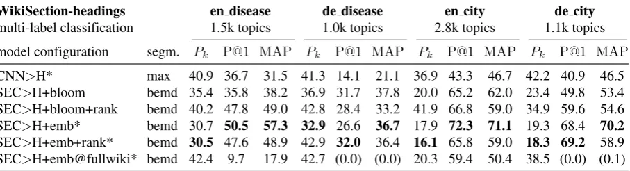
WikiSection-headings
multi-label classification
en disease
1.5k topics
de disease
1.0k topics
en city
2.8k topics
de city
1.1k topics model configuration segm. Pk P@1 MAP Pk P@1 MAP Pk P@1 MAP Pk P@1 MAP
CNN>H* max 40.9 36.7 31.5 41.3 14.1 21.1 36.9 43.3 46.7 42.2 40.9 46.5 SEC>H+bloom bemd 35.4 35.8 38.2 36.9 31.7 37.8 20.0 65.2 62.0 23.4 49.8 53.4 SEC>H+bloom+rank bemd 40.2 47.8 49.0 42.8 28.4 33.2 41.9 66.8 59.0 34.9 59.6 54.6 SEC>H+emb* bemd 30.7 50.5 57.3 32.9 26.6 36.7 17.9 72.3 71.1 19.3 68.4 70.2
SEC>H+emb+rank* bemd 30.5 47.6 48.9 42.9 32.0 36.4 16.1 65.8 59.0 18.3 69.2 58.9 SEC>H+emb@fullwiki* bemd 42.4 9.7 17.9 42.7 (0.0) (0.0) 20.3 59.4 50.4 38.5 (0.0) (0.1)
Table 4: Results for segmentation and multi-label classification trained with raw Wikipedia headings. Here, the task is to segment the document and predict multi-word topics from a large ambiguous target vocabulary.
model training and inference using pre-trained embeddings is faster by an average factor of 3.2.
Topic Embeddings Perform Well on Noisy Data. In the multi-label setting with unprocessed Wikipedia headings, classification precision of SECTORreaches up to 72.3% P@1 for 2.8k labels. This score is in average 9.5 points lower compared to the models trained on the small number of 25–30 normalized labels. Furthermore, segmentation performance only misses 3.8 pointsPkcompared
with the topics task. Ranking loss could not
improve our models significantly, but achieved better segmentation scores on the headings task. Finally, the cross-domain Englishfullwikimodel performs only on baseline level for segmentation, but still achieves better classification performance than CNN on the English cities data set.
5.2 Discussion and Model Insights
[image:11.595.75.529.424.547.2]Segmentation Wiki-50 Cities Elements Clinical
and multi-label classification Pk MAP Pk MAP Pk MAP Pk
GraphSeg 63.6 n/a 40.0 n/a 49.1 n/a −
BayesSeg 49.2 n/a 36.2 n/a 35.6 n/a 57.8
TextSeg 18.2* n/a 19.7* n/a 41.6 n/a 30.8
SEC>H+emb@en disease − − − − 43.3 9.5 36.5
SEC>C+emb@en disease − − − − 45.1 n/a 35.6
[image:12.595.123.474.58.204.2]SEC>H+emb@en city 30.0 31.4 28.2 56.5 41.0 7.9 − SEC>C+emb@en city 31.3 n/a 22.9 n/a 48.8 n/a − SEC>H+emb@cities 33.3 15.3 21.4* 52.3* 39.2 12.1 37.7 SEC>H+emb@fullwiki 28.6* 32.6* 33.4 40.5 42.8 14.4 36.9
Table 5: Results for cross-data set evaluation on existing data sets. Numbers marked with * are generated by models trained specifically for this data set. A value of ‘n/a’ indicates that a model is not applicable to this problem.
inf scr man epi com trea prev diag cau sym
sym cau ... diag prev ... trea com epi inf
scr man epi com trea prev diag cau sym
sym cau ... diag prev ... trea com epi
pro scr pat epi com trea prev diag cau sym
sym cau ... diag prev ... trea com epi pro
scr pat epi com trea prev diag cau sym
sym cau ... diag prev ... trea com epi PV>T (NL)
SEC>T+bloom (NL)
PV>T (emd)
SEC>T+bloom (bemd)
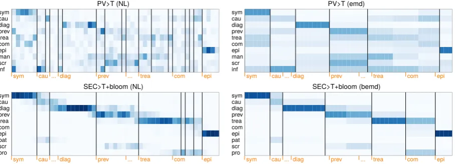
Figure 5: Heatmaps of predicted topic labelsˆykfor documentTrichomoniasisfrom PV and SECTORmodels with newline and embedding segmentation. Shading denotes probability for 10 out of 27 selected topic classes onY axis, with sentences from left to right. Segmentation is shown as black lines,X axis shows expected gold labels. Note that segments with same class assignments are merged in both predictions and gold standard (‘. . . ’).
SECTOR Captures Latent Topics from Context.
We clearly see from NL predictions (left side of Figure 5) that SECTOR produces coherent results with sentence granularity, with topics emerging and disappearing over the course of a document. In contrast, PV predictions are scat-tered across the document. Both models success-fully classify first (symptoms) and last sections
(epidemiology). However, only SECTORcan
cap-ture diagnosis, prevention, and treatment.
Furthermore, we observe additionalscreening
predictions in the center of the document. This section is actually labeled "Prevention |
Screening" in the source document, which
explains this overlap.
Furthermore, we observe low confidence in the second section labeled cause. Our multi-class model predicts for this section {diagnosis,
cause, genetics}. The ground truth heading
for this section is "Causes | Genetic
sequence," but even for a human reader this
assignment is not clear. This shows that the multi-label approach fills an important gap and can even serve as an indicator for low-quality article structure.
Finally, both models fail to segment the
com-plication section near the end, because it
[image:12.595.74.528.262.426.2]6 Conclusions and Future Work
We presented SECTOR, a novel model for coherent text segmentation and classification based on latent topics. We further contributed WIKISECTION, a collection of four large data sets in English and German for this task. Our end-to-end method builds on a neural topic embedding which is trained using Wikipedia headings to optimize a bidirectional LSTM classifier. We showed that our best performing model is based on sparse word features with Bloom filter encoding and significantly improves classification precision for 25–30 topics on comprehensive documents by up to 29.5 points F1 compared with state-of-the-art sentence classifiers with baseline segmentation. We used the bidirectional deviation in our topic embedding to segment a document into coherent sections without additional training. Finally, our experiments showed that extending the task to multi-label classification of 2.8k ambiguous topic words still produces coherent results with 71.1% average precision.
We see an exciting future application ofSECTOR as a building block to extract and retrieve topical passages from unlabeled corpora, such as medical research articles or technical papers. One possible task is WikiPassageQA (Cohen et al., 2018), a benchmark to retrieve passages as answers to non-factoid questions from long articles.
Acknowledgments
We would like to thank the editors and anonymous reviewers for their helpful suggestions and comments. Our work is funded by the German Federal Ministry of Economic Affairs and Energy (BMWi) under grant agreement 01MD16011E (Medical Allround-Care Service Solutions) and H2020 ICT-2016-1 grant agreement 732328 (FashionBrain).
References
Shashank Agarwal and Hong Yu. 2009. Auto-matically classifying sentences in full-text biomedical articles into introduction, meth-ods, results and discussion. Bioinformatics, 25(23):3174–3180.
Yamen Ajjour, Wei-Fan Chen, Johannes Kiesel, Henning Wachsmuth, and Benno Stein. 2017.
Unit segmentation of argumentative texts. In Proceedings of the 4th Workshop on Argument Mining, pages 118–128.
Alexander A. Alemi and Paul Ginsparg. 2015. Text segmentation based on semantic word embeddings.CoRR, cs.CL/1503.05543v1. James Allan. 2002, Introduction to topic detection
and tracking. InTopic Detection and Tracking, pages 1–16. Springer.
Loulwah AlSumait, Daniel Barbar´a, and Carlotta Domeniconi. 2008. On-line LDA: Adaptive topic models for mining text streams with applications to topic detection and tracking. In Eighth IEEE International Conference on Data Mining, pages 3–12. IEEE.
Sanjeev Arora, Yingyu Liang, and Tengyu Ma. 2017. A simple but tough-to-beat baseline for sentence embeddings. In ICLR 2017: 5th International Conference on Learning Representations.
M. Bayomi, K. Levacher, M. R. Ghorab, and S. Lawless. 2015. OntoSeg: A novel approach to text segmentation using ontological similarity. In 2015 International Conference on Data Mining Workshop, pages 1274–1283. IEEE. Doug Beeferman, Adam Berger, and John
Lafferty. 1999. Statistical models for text seg-mentation.Machine Learning, 34(1):177–210. Shraey Bhatia, Jey Han Lau, and Timothy
Baldwin. 2016. Automatic labelling of topics with neural embeddings. InProceedings of the 26th International Conference on Computa-tional Linguistics, pages 953–963.
David M. Blei, Andrew Y. Ng, and Michael I. Jordan. 2003. Latent dirichlet allocation. Jour-nal of Machine Learning Research, 3(Jan): 993–1022.
Freddy Y. Y. Choi. 2000. Advances in do-main independent linear text segmentation. In Proceedings of the 1st North American Chapter of the Association for Computational Linguistics Conference, pages 26–33. ACL. Philipp Cimiano, Antje Schultz, Sergej Sizov,
Philipp Sorg, and Steffen Staab. 2009. Explicit versus latent concept models for cross-language information retrieval. In Proceedings of the 21st International Joint Conference on Artifical Intelligence, volume 9, pages 1513–1518. Daniel Cohen, Liu Yang, and W. Bruce Croft.
2018. WikiPassageQA: A benchmark collection for research on non-factoid answer passage retrieval. InThe 41st International ACM SIGIR Conference on Research & Development in Information Retrieval, pages 1165–1168. ACM. Alexis Conneau, Holger Schwenk, Lo¨ıc Barrault, and Yann Lecun. 2017. Very deep convolu-tional networks for text classification. In Proceed-ings of the 15th Conference of the European Chapter of the Association for Computa-tional Linguistics, volume 1, pages 1107–1116. ACL.
Ga¨el Dias, Elsa Alves, and Jos´e Gabriel Pereira Lopes. 2007. Topic segmentation algorithms for text summarization and passage retrieval: An exhaustive evaluation. InProceedings of the Twenty-Second AAAI Conference on Artificial Intelligence, volume 7, pages 1334–1340. Adji B. Dieng, Chong Wang, Jianfeng Gao, and
John Paisley. 2017. TopicRNN: A recurrent neural network with long-range semantic de-pendency. In ICLR 2017: 5th International Conference on Learning Representations. Lan Du, Wray Buntine, and Mark Johnson.
2013. Topic segmentation with a structured topic model. In Proceedings of the 2013 Conference of the North American Chapter of the Asso-ciation for Computational Linguistics: Human Language Technologies, pages 190–200. Jacob Eisenstein and Regina Barzilay. 2008.
Bayesian unsupervised topic segmentation. In Proceedings of the 2008 Conference on Empir-ical Methods in Natural Language Process-ing, pages 334–343. ACL.
George W. Furnas, Thomas K. Landauer, Louis M. Gomez, and Susan T. Dumais. 1987. The vocabulary problem in human-system com-munication. Communications of the ACM, 30(11):964–971.
Evgeniy Gabrilovich and Shaul Markovitch. 2007. Computing semantic relatedness using Wikipedia-based explicit semantic analysis. In Proceedings of the Twentieth International Joint Conference on Artificial Intelligence, pages 1606–1611.
Felix A. Gers, J¨urgen A. Schmidhuber, and Fred A. Cummins. 2000. Learning to forget: Continual prediction with LSTM.Neural Compututation, 12(10):2451–2471.
Goran Glavaˇs, Federico Nanni, and Simone Paolo Ponzetto. 2016. Unsupervised text segmen-tation using semantic relatedness graphs. In Proceedings of the Fifth Joint Conference on Lexical and Computational Semantics, pages 125–130. ACL.
Alex Graves. 2012.Supervised Sequence Labelling with Recurrent Neural Networks, volume 385, Springer, Berlin Heidelberg.
Marti A. Hearst. 1997. TextTiling: Segmenting text into multi-paragraph subtopic passages. Computational Linguistics, 23(1):33–64. Daniel Hewlett, Alexandre Lacoste, Llion Jones,
Illia Polosukhin, Andrew Fandrianto, Jay Han, Matthew Kelcey, and David Berthelot. 2016. WikiReading: A novel large-scale lang-uage understanding task over Wikipedia. In Proceedings of the 54th Annual Meeting of the Association for Computational Linguistics, volume 1, pages 1535–1545. ACL.
Felix Hill, Kyunghyun Cho, and Anna Korhonen. 2016. Learning distributed representations of sentences from unlabelled data. InProceedings of the 2016 Conference of the North American Chapter of the Association for Computational Linguistics: Human Language Technologies, pages 1367–1377.
Hoa T. Le, Christophe Cerisara, and Alexandre Denis. 2018. Do convolutional networks need to be deep for text classification? InAssociation for the Advancement of Artificial Intelligence 2018 Workshop on Affective Content Analysis, pages 29–36.
Sepp Hochreiter and J¨urgen Schmidhuber. 1997. Long short-term memory.Neural Computation, 9(8):1735–1780.
Xiangji Huang, Fuchun Peng, Dale Schuurmans, Nick Cercone, and Stephen E. Robertson. 2003. Applying machine learning to text segmentation for information retrieval.Information Retrieval, 6(3-4):333–362.
Minwoo Jeong and Ivan Titov. 2010. Multi-document topic segmentation. In Proceedings of the 19th ACM International Conference on Information and Knowledge Management, pages 1119–1128. ACM.
Bin Jiang. 2012. Head/tail breaks: A new classifi-cation scheme for data with a heavy-tailed distribution. The Professional Geographer, 65(3):482–494.
Hubert Jin, Rich Schwartz, Sreenivasa Sista, and Frederick Walls. 1999. Topic tracking for radio, TV broadcast and newswire. In Proceedings of the DARPA Broadcast News Workshop, pages 199–204. Morgan Kaufmann.
Thorsten Joachims. 1998. Text categorization with support vector machines: Learning with many relevant features. In European Conference on Machine Learning, pages 137–142. Springer. Yoon Kim. 2014. Convolutional neural networks
for sentence classification. In Proceedings of the 2014 Conference on Empirical Methods in Natural Language Processing, pages 1746–1751.
Omri Koshorek, Adir Cohen, Noam Mor, Michael Rotman, and Jonathan Berant. 2018. Text segmentation as a supervised learning task. In Proceedings of the 2018 Conference of the North American Chapter of the Association for Computational Linguistics: Human Language Technologies, Volume 2 (Short Papers), volume 2, pages 469–473.
Giridhar Kumaran and James Allan. 2004. Text classification and named entities for new event detection. In Proceedings of the 27th Annual International ACM SIGIR Conference on Research and Development in Information Retrieval, pages 297–304. ACM.
Quoc V. Le and Tomas Mikolov. 2014. Distrib-uted representations of sentences and docu-ments. InProceedings of the 31st International Conference on Machine Learning, volume 32, pages 1188–1196.
Yann LeCun, Sumit Chopra, Raia Hadsell, M. Ranzato, and F. Huang. 2006, A tutorial on energy-based learning. InPredicting Structured Data, volume 1, MIT.
Kalev Leetaru and Philip A. Schrodt. 2013. GDELT: Global data on events, location, and tone, 1979–2012. In ISA Annual Convention, volume 2, pages 1–49. Citeseer.
Jialu Liu, Xiang Ren, Jingbo Shang, Taylor Cassidy, Clare R. Voss, and Jiawei Han. 2016. Representing documents via latent key-phrase inference. In Proceedings of the 25th International Conference on World Wide Web, pages 1057–1067.
Xiaoyong Liu and W. Bruce Croft. 2002. Passage retrieval based on language models. In Proceedings of the Eleventh International Conference on Information and Knowledge Management, pages 375–382. ACM.
Sean MacAvaney, Andrew Yates, Arman Cohan, Luca Soldaini, Kai Hui, Nazli Goharian, and Ophir Frieder. 2018. Characterizing question facets for complex answer retrieval. In The 41st International ACM SIGIR Conference on Research & Development in Information Retrieval, pages 1205–1208. ACM Press. Tomas Mikolov, Kai Chen, Greg Corrado, and
Jeffrey Dean. 2013. Efficient estimation of word representations in vector space. CoRR, cs.CL/1301.3781v3.
Intelligent Information & Engineering Sys-tems, volume 112 of Procedia Computer Science, pages 340–349. Elsevier.
Federico Nanni, Bhaskar Mitra, Matt Magnusson, and Laura Dietz. 2017. Benchmark for complex answer retrieval. In Proceedings of the ACM SIGIR International Conference on Theory of Information Retrieval, pages 293–296. ACM. Roberto Navigli and Simone Paolo Ponzetto.
2012. BabelNet: The automatic construction, evaluation and application of a wide-coverage multilingual semantic network. Artificial Intelligence, 193:217–250.
Mark E. J. Newman. 2006. Finding community structure in networks using the eigenvectors of matrices.Physical Review E, 74(3):036104. Tiziano Piccardi, Michele Catasta, Leila Zia,
and Robert West. 2018. Structuring Wikipedia articles with section recommendations. In Pro-ceedings of the 41th International ACM SIGIR Conference on Research and Development in Information Retrieval, pages 665–674. ACM. Yashoteja Prabhu and Manik Varma. 2014.
FastXML: A fast, accurate and stable tree-classifier for extreme multi-label learning. In Proceedings of the 20th ACM SIGKDD Inter-national Conference on Knowledge Discovery and Data Mining, pages 263–272. ACM. Martin Riedl and Chris Biemann. 2012.
Topic-Tiling: A text segmentation algorithm based on LDA. In Proceedings of ACL 2012 Student Research Workshop, pages 37–42. ACL. Cicero Nogueira dos Santos, Bing Xiang, and
Bowen Zhou. 2015. Classifying relations by ranking with convolutional neural networks. In Proceedings of the 53rd Annual Meeting of the Association for Computational Linguistics and the 7th International Joint Conference on Nat-ural Language Processing, pages 626–634. ACL. Imran Sehikh, Dominique Fohr, and Irina Illina. 2017. Topic segmentation in ASR transcripts using bidirectional RNNs for change detection. In Automatic Speech Recognition and Under-standing Workshop, pages 512–518. IEEE. Joan Serr`a and Alexandros Karatzoglou. 2017.
Getting deep recommenders fit: Bloom
embed-dings for sparse binary input/output networks. In Proceedings of the Eleventh ACM Conference on Recommender Systems, pages 279–287. ACM. Thomas Pellissier Tanon, Denny Vrandecic, Sebastian Schaffert, Thomas Steiner, and Lydia Pintscher. 2016. From Freebase to Wikidata: The great migration. InProceedings of the 25th International Conference on World Wide Web, pages 1419–1428.
Michael Tepper, Daniel Capurro, Fei Xia, Lucy Vanderwende, and Meliha Yetisgen-Yildiz. 2012. Statistical section segmentation in free-text clinical records. In Proceedings of the Eighth International Conference on Language Resources and Evaluation, pages 2001–2008. George Tsatsaronis, Michael Schroeder, Georgios
Paliouras, Yannis Almirantis, Ion Androutsopoulos, Eric Gaussier, Patrick Gallinari, Thierry Artieres, Michael R. Alvers, and Matthias Zschunke. 2012. BioASQ: A challenge on large-scale biomedical semantic indexing and question answering. InAAAI Technical Report FS-12-05 Information Retrieval and Knowledge Discovery in Biomedical Text, pages 92–98. Grigorios Tsoumakas, Ioannis Katakis, and
Ioannis Vlahavas. 2009. Mining multi-label data. InData Mining and Knowledge Discovery Handbook, pages 667–685. Springer.
Masao Utiyama and Hitoshi Isahara. 2001. A statistical model for domain-independent text segmentation. In Proceedings of the 39th Annual Meeting on Association for Compu-tational Linguistics, pages 499–506. ACL. Liang Wang, Sujian Li, Yajuan Lyu, and Houfeng
Wang. 2017. Learning to rank semantic co-herence for topic segmentation. In Proceed-ings of the 2017 Conference on Empirical Methods in Natural Language Processing, pages 1340–1344. ACL.
Jui-Feng Yeh, Yi-Shan Tan, and Chen-Hsien Lee. 2016. Topic detection and tracking for conversational content by using con-ceptual dynamic latent Dirichlet allocation. Neurocomputing, 216:310–318.