Minibatch and Parallelization for Online Large Margin Structured Learning

Minibatch and Parallelization for Online Large Margin Structured Learning

Kai Zhao1

1_{Computer Science Program, Graduate Center}

City University of New York [email protected]

Liang Huang2,1

2_{Computer Science Dept, Queens College}

City University of New York [email protected]

Abstract

Online learning algorithms such as perceptron and MIRA have become popular for many NLP tasks thanks to their simpler architec-ture and faster convergence over batch learn-ing methods. However, while batch learnlearn-ing such as CRF is easily parallelizable, online learning is much harder to parallelize: previ-ous efforts often witness a decrease in the con-verged accuracy, and the speedup is typically very small (∼3) even with many (10+) pro-cessors. We instead present a much simpler architecture based on “mini-batches”, which is trivially parallelizable. We show that, un-like previous methods, minibatch learning (in serial mode) actuallyimprovesthe converged accuracy for both perceptron and MIRA learn-ing, and when combined with simple paral-lelization, minibatch leads to very significant speedups (up to 9x on 12 processors) on state-of-the-art parsing and tagging systems.

1 Introduction

Online structured learning algorithms such as the structured perceptron (Collins, 2002) and k-best MIRA (McDonald et al., 2005) have become more and more popular for many NLP tasks such as de-pendency parsing and part-of-speech tagging. This is because, compared to their batch learning counter-parts, online learning methods offer faster conver-gence rates and better scalability to large datasets, while using much less memory and a much simpler architecture which only needs 1-best or k-best de-coding. However, online learning for NLP typically involves expensive inference on each example for 10 or more passes over millions of examples, which of-ten makes training too slow in practice; for example systems such as the popular (2nd-order) MST parser

(McDonald and Pereira, 2006) usually require the order of days to train on the Treebank on a com-modity machine (McDonald et al., 2010).

There are mainly two ways to address this scala-bility problem. On one hand, researchers have been developing modified learning algorithms that allow inexact search (Collins and Roark, 2004; Huang et al., 2012). However, the learner still needs to loop over the whole training data (on the order of mil-lions of sentences) many times. For example the best-performing method in Huang et al. (2012) still requires 5-6 hours to train a very fast parser.

On the other hand, with the increasing popularity of multicore and cluster computers, there is a grow-ing interest in speedgrow-ing up traingrow-ing via paralleliza-tion. While batch learning such as CRF (Lafferty et al., 2001) is often trivially parallelizable (Chu et al., 2007) since each update is a batch-aggregate of the update from each (independent) example, online learning is much harder to parallelize due to the de-pendency between examples, i.e., the update on the first example should in principle influence the coding of all remaining examples. Thus if we de-code and update the first and the 1000th examples in parallel, we lose their interactions which is one of the reasons for online learners’ fast convergence. This explains why previous work such as the itera-tive parameter mixing (IPM) method of McDonald et al. (2010) witnesses a decrease in the accuracies of parallelly-learned models, and the speedup is typ-ically very small (about 3 in their experiments) even with 10+ processors.

We instead explore the idea of “minibatch” for on-line large-margin structured learning such as percep-tron and MIRA. We argue that minibatch is advan-tageous inbothserial and parallel settings.

First, for minibatch perceptron in the serial

ting, our intuition is that, although decoding is done independently within one minibatch, updates are done by averaging update vectors in batch, provid-ing a “mixprovid-ing effect” similar to “averaged parame-ters” of Collins (2002) which is also found in IPM (McDonald et al., 2010), and online EM (Liang and Klein, 2009).

Secondly, minibatch MIRA in the serial setting has an advantage that, different from previous meth-ods such as SGD which simply sum up the up-dates from all examples in a minibatch, a minibatch MIRA update tries to simultaneously satisfy an ag-gregated set of constraints that are collected from multiple examples in the minibatch. Thus each mini-batch MIRA update involves an optimization over many more constraints than in pure online MIRA, which could potentially lead to a better margin. In other words we can view MIRA as an online version or stepwise approximation of SVM, and minibatch MIRA can be seen as a better approximation as well as a middleground between pure MIRA and SVM.1

More interestingly, the minibatch architecture is trivially parallelizable since the examples within each minibatch could be decoded in parallel on mul-tiple processors (while the update is still done in se-rial). This is known as “synchronous minibatch” and has been explored by many researchers (Gim-pel et al., 2010; Finkel et al., 2008), but all previ-ous works focus on probabilistic models along with SGD or EM learning methods while our work is the first effort on large-margin methods.

We make the following contributions:

• Theoretically, we present a serial minibatch framework (Section 3) for online large-margin learning and prove the convergence theorems for minibatch perceptron and minibatch MIRA.

• Empirically, we show that serial minibatch could speed up convergence and improve the converged accuracy for both MIRA and percep-tron on state-of-the-art dependency parsing and part-of-speech tagging systems.

• In addition, when combined with simple (syn-chronous) parallelization, minibatch MIRA

1

This is similar to Pegasos (Shalev-Shwartz et al., 2007) that applies subgradient descent over a minibatch. Pegasos becomes pure online when the minibatch size is1.

Algorithm 1Generic Online Learning.

Input: dataD={(x(t)_{, y}(t)_)}n

t=1and feature mapΦ Output: weight vectorw

1: repeat

2: for eachexample(x, y)inDdo

3: C←FINDCONSTRAINTS(x, y,w).decoding 4: ifC6=∅thenUPDATE(w, C)

5: untilconverged

leads to very significant speedups (up to 9x on 12 processors) that are much higher than that of IPM (McDonald et al., 2010) on state-of-the-art parsing and tagging systems.

2 Online Learning: Perceptron and MIRA

We first present a unified framework for online large-margin learning, where perceptron and MIRA are two special cases. Shown in Algorithm 1, the online learner considers each input example (x, y) sequentially and performs two steps:

1. find the setCof violating constraints, and

2. update the weight vectorwaccording toC.

Here a triplehx, y, ziis said to be a “violating con-straint” with respect to modelwif the incorrect la-bel z scores higher than (or equal to) the correct label y in w, i.e., w·∆Φ(hx, y, zi) ≤ 0, where ∆Φ(hx, y, zi) is a short-hand notation for the up-date vectorΦ(x, y)−Φ(x, z) andΦis the feature map (see Huang et al. (2012) for details). The sub-routines FINDCONSTRAINTSand UPDATEare anal-ogous to “APIs”, to be specified by specific instances of this online learning framework. For example, the structured perceptron algorithm of Collins (2002) is implemented in Algorithm 2 where FINDCON -STRAINTSreturns a singleton constraint if the 1-best decoding resultz(the highest scoring label accord-ing to the current model) is different from the true labely. Note that in the UPDATE function,C is al-ways a singleton constraint for the perceptron, but we make it more general (as a set) to handle the batch update in the minibatch version in Section 3.

Algorithm 2Perceptron (Collins, 2002). 1: functionFINDCONSTRAINTS(x, y,w)

2: z←argmax_s∈Y(x)w·Φ(x, s) .decoding 3: ifz6=ythen return{hx, y, zi}

4: else return∅

5: procedureUPDATE(w, C) 6: w←w+_|C1_|P

c∈C∆Φ(c) .(batch) update

Algorithm 3k-best MIRA (McDonald et al., 2005). 1: functionFINDCONSTRAINTS(x, y,w)

2: Z ←k-bestz∈Y(x)w·Φ(x, z)

3: Z ← {z∈Z |z6=y,w·∆Φ(hx, y, zi)≤0}

4: return{(hx, y, zi, `(y, z))|z∈Z}

5: procedureUPDATE(w, C)

6: w← argmin

w0_{:∀(c,`)∈C,w</sub>0<sub>·∆Φ(c)≥`}

kw0_−wk2

finds thek-best solutions Z first, and returns a set of violating constraints inZ, The update in MIRA is more interesting: it searches for the new model

w0 with minimum change from the current model

w so that w0 corrects each violating constraint by a margin at least as large as the loss`(y, z) of the incorrect labelz.

Although not mentioned in the pseudocode, we also employ “averaged parameters” (Collins, 2002) for both perceptron and MIRA in all experiments.

3 Serial Minibatch

The idea of serial minibatch learning is extremely simple: divide the data into dn/me minibatches of size m, and do batch updates after decoding each minibatch (see Algorithm 4). The FIND -CONSTRAINTSand UPDATEsubroutines remain un-changed for both perceptron and MIRA, although it is important to note that a perceptron batch up-date uses the average of upup-date vectors, not the sum, which simplifies the proof. This architecture is of-ten called “synchronous minibatch” in the literature (Gimpel et al., 2010; Liang and Klein, 2009; Finkel et al., 2008). It could be viewed as a middleground between pure online learning and batch learning.

3.1 Convergence of Minibatch Perceptron

We denoteC(D)to be the set of all possible violat-ing constraints in dataD(cf. Huang et al. (2012)):

C(D) ={hx, y, zi |(x, y)∈D, z∈ Y(x)− {y}}.

Algorithm 4Serial Minibatch Online Learning.

Input: dataD, feature mapΦ, and minibatch sizem Output: weight vectorw

1: SplitDintodn/meminibatchesD1. . . Ddn/me

2: repeat

3: fori←1. . .dn/medo .for each minibatch 4: C← ∪(x,y)∈DiFINDCONSTRAINTS(x, y,w)

5: ifC6=∅thenUPDATE(w, C) .batch update 6: untilconverged

A training set Disseparable by feature mapΦ

withmarginδ >0if there exists a unit oracle vec-toruwithkuk= 1such thatu·∆Φ(hx, y, zi)≥δ, for all hx, y, zi ∈ C(D). Furthermore, let radius

R≥ k∆Φ(hx, y, zi)kfor allhx, y, zi ∈C(D).

Theorem 1. For a separable datasetDwith margin δand radiusR, the minibatch perceptron algorithm (Algorithms 4 and 2) will terminate aftertminibatch updates wheret≤R2/δ2.

Proof. Let wt _{be the weight vector beforethe t}th

update; w0 = 0. Suppose the tth update happens on the constraint set Ct = {c1, c2, . . . , ca} where

a = |Ct|, and each ci = hxi, yi, zii. We convert them to the set of update vectorsvi = ∆Φ(ci) = ∆Φ(hxi, yi, zii)for alli. We know that:

1. u·vi≥δ (margin on unit oracle vector)

2. wt_·v

i ≤0 (violation:zidominatesyi)

3. kvik2 ≤R2 (radius)

Now the update looks like

wt+1=wt+ 1

|Ct|

X

c∈Ct

∆Φ(c) =wt+1 a

P

ivi.

(1) We will boundkwt+1kfrom two directions:

1. Dot product both sides of the update equa-tion (1) with the unit oracle vectoru, we have

u·wt+1=u·wt + 1

a P

iu·vi

≥u·wt + 1

a P

iδ (margin)

=u·wt + δ (P

i =a)

Since for any two vectors a and b we have

kakkbk ≥a·b, thuskukkwt+1k ≥u·wt+1≥ tδ. Asuis a unit vector, we havekwt+1_{k ≥tδ.}

2. On the other hand, take the norm of both sides of Eq. (1):

kwt+1k2=kwt+1 a

P

ivik2

=kwtk2+kP

i 1avik2+ 2

a w

t_·P

ivi

≤kwtk2_+kP

i 1avik

2_{+ 0 (violation)}

≤kwtk2+P

i

1

akvik2 (Jensen’s)

≤kwtk2₊P

ia1R

2 _(radius)

=kwtk2+R2 (P

i =a)

≤tR2 (by induction)

Combining the two bounds, we have

t2δ2 ≤ kwt+1k2≤tR2

thus the number of minibatch updates t ≤ R2_/δ2_.

Note that this bound is identical to that of pure online perceptron (Collins, 2002, Theorem 1) and is irrelevant to minibatch sizem. The use of Jensen’s inequality is inspired by McDonald et al. (2010).

3.2 Convergence of Minibatch MIRA

We also give a proof of convergence for MIRA with relaxation.2We present the optimization problem in the UPDATEfunction of Algorithm 3 as a quadratic program (QP) with slack variableξ:

wt+1 ←argmin

wt+1

kwt+1−wtk2_+ξ

s.t.wt+1·vi≥`i−ξ, for all(ci, `i)∈Ct

where vi = ∆Φ(ci) is the update vector for con-straintci. Consider the Lagrangian:

L=kwt+1−wtk2+ξ+

|Ct|

X

i=1

ηi(`i−w0·vi−ξ)

ηi ≥0, for1≤i≤ |Ct|.

2

Actually this relaxation is not necessary for the conver-gence proof. We employ it here solely to make the proof shorter. It isnotused in the experiments either.

Set the partial derivatives to0with respect tow0and

ξwe have:

w0 =w+P

iηivi (2)

P

iηi = 1 (3)

This result suggests that the weight change can al-ways be represnted by a linear combination of the update vectors (i.e. normal vectors of the constraint hyperplanes), with the linear coefficencies sum to1.

Theorem 2(convergence of minibatch MIRA). For a separable datasetDwith marginδand radiusR, the minibatch MIRA algorithm (Algorithm 4 and 3) will maketupdates wheret≤R2/δ2.

Proof. 1. Dot product both sides of Equation 2 with unit oracle vectoru:

u·wt+1=u·wt + P

iηiu·vi

≥u·wt + P

iηiδ (margin) =u·wt + δ (Eq. 3)

=tδ (by induction)

2. On the other hand

kwt+1k2 _=kwt₊P

iηivik2 =kwtk2+kP

iηivik2+ 2w t_·P

iηivi

≤kwtk2_+kP

iηivik2+ 0 (violation)

≤kwtk2+P

iηiv2i (Jensen’s)

≤kwtk2+P

iηiR2 (radius) =kwtk2+R2 (Eq. 3)

≤tR2 (by induction)

From the two bounds we have:

t2δ2 ≤ kwt+1k2≤tR2

thus within at mostt ≤ R2/δ2 minibatch up-dates MIRA will converge.

4 Parallelized Minibatch

update 1

3

4 2

update update update

6 5

8 7 update

update update

update 12 9

10

11 update

update

update update

15 14 13

16 update update

update

update

⊕

update 3

1 4

6 5

8 7

2

12

15 14

9 13

16 10

11 ⊕

update⊕

3

1 4

6 5

8 7

2

12

15 14

9

13

16 10

11 update⊕

update⊕

update 1

2 3 4

6 5

8 7

update

update 9

10

update ₁₂

11

14 13

15

16

update update

update

update

(a) IPM (b) unbalanced (c) balanced (d) asynchronous

Figure 1: Comparison of various methods for parallelizing online learning (number of processorsp= 4). (a) iterative parameter mixing (McDonald et al., 2010). (b) unbalanced minibatch parallelization (minibatch sizem = 8). (c) minibatch parallelization after load-balancing (within each minibatch). (d) asynchronous minibatch parallelization (Gimpel et al., 2010) (not implemented here). Each numbered box denotes the decoding of one example, and⊕

denotes an aggregate operation, i.e., the merging of constraints after each minibatch or the mixing of weights after each iteration in IPM. Each gray shaded box denotes time wasted due to synchronization in (a)-(c) or blocking in (d). Note that in (d) at most one update can happen concurrently, making it substantially harder to implement than (a)-(c).

Algorithm 5Parallized Minibatch Online Learning.

Input:D,Φ, minibatch sizem, and # of processorsp Output: weight vectorw

SplitDintodn/meminibatchesD1. . . Ddn/me Split eachDiintom/pgroupsDi,1. . . Di,m/p

repeat

fori←1. . .dn/medo .for each minibatch

forj←1. . . m/pin parallel do

Cj← ∪(x,y)∈Di,jFINDCONSTRAINTS(x, y,w)

C← ∪jCj .in serial

ifC6=∅thenUPDATE(w, C) .in serial

untilconverged

other examples in the same batch. Thus we can eas-ily distribute decoding for different examples in the same minibatch to different processors.

Shown in Algorithm 5, for each minibatchDi, we split Di into groups of equal size, and assign each group to a processor to decode. After all processors finish, we collect all constraints and do an update based on the union of all constraints. Figure 1 (b) il-lustrates minibatch parallelization, with comparison to iterative parameter mixing (IPM) of McDonald et al. (2010) (see Figure 1 (a)).

This synchronous parallelization framework should provide significant speedups over the serial

mode. However, in each minibatch, inevitably, some processors will end up waiting for others to finish, especially when the lengths of sentences vary substantially (see the shaded area in Figure 1 (b)).

To alleviate this problem, we propose “ per-minibatch load-balancing”, which rearranges the sentences within each minibatch based on their lengths (which correlate with their decoding times) so that the total workload on each processor is bal-anced (Figure 1c). It is important to note that this shuffling doesnotaffect learning at all thanks to the independence of each example within a minibatch. Basically, we put the shortest and longest sentences into the first thread, the second shortest and second longest into the second thread, etc. Although this is not necessary optimal scheduling, it works well in practice. As long as decoding time is linear in the length of sentence (as in incremental parsing or tag-ging), we expect a much smaller variance in process-ing time on each processor in one minibatch, which is confirmed in the experiments (see Figure 8).3

3

5 Experiments

We conduct experiments on two typical structured prediction problems: incremental dependency pars-ing and part-of-speech taggpars-ing; both are done on state-of-the-art baseline. We also compare our parallelized minibatch algorithm with the iterative parameter mixing (IPM) method of McDonald et al. (2010). We perform our experiments on a commodity 64-bit Dell Precision T7600 worksta-tion with two 3.1GHz 8-core CPUs (16 processors in total) and 64GB RAM. We use Python 2.7’s multiprocessingmodule in all experiments.4

5.1 Dependency Parsing with MIRA

We base our experiments on our dynamic program-ming incremental dependency parser (Huang and Sagae, 2010).5 Following Huang et al. (2012), we use max-violation update and beam sizeb = 8. We evaluate on the standard Penn Treebank (PTB) us-ing the standard split: Sections 02-21 for trainus-ing, and Section 22 as the held-out set (which is indeed the test-set in this setting, following McDonald et al. (2010) and Gimpel et al. (2010)). We then ex-tend it to employ 1-best MIRA learning. As stated in Section 2, MIRA separates the gold labelyfrom the incorrect labelz with a margin at least as large as the loss`(y, z). Here in incremental dependency parsing we define the loss function between a gold treey and an incorrectpartialtreezas the number of incorrect edges in z, plus the number of correct edges iny which are already ruled out by z. This MIRA extension results in slightly higher accuracy of 92.36, which we will use as the pure online learn-ing baseline in the comparisons below.

5.1.1 Serial Minibatch

We first run minibatch in the serial mode with varying minibatch size of 4, 16, 24, 32, and 48 (see Figure 2). We can make the following observations. First, except for the largest minibatch size of 48, minibatch learning generally improves the accuracy

4

Weturn off garbage-collectionin worker processes oth-erwise their running times will be highly unbalanced. We also admit that Python is not the best choice for parallelization, e.g., asychronous minibatch (Gimpel et al., 2010) requires “shared memory” not found in the current Python (see also Sec. 6).

5_{Available athttp://acl.cs.qc.edu/. The version}

with minibatch parallelization will be available there soon.

90.75 91 91.25 91.5 91.75 92 92.25 92.5

0 1 2 3 4 5 6 7 8

accuracy on held-out

wall-clock time (hours) m=1 m=4 m=16 m=24 m=32 m=48

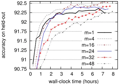
Figure 2: Minibatch with various minibatch sizes (m= 4,16,24,32,48) for parsing with MIRA, compared to pure MIRA (m = 1). All curves are on a single CPU.

of the converged model, which is explained by our intuition that optimization with a larger constraint set could improve the margin. In particular,m= 16 achieves the highest accuracy of 92.53, which is a 0.27 improvement over the baseline.

Secondly, minibatch learning can reach high lev-els of accuracy faster than the baseline can. For ex-ample, minibatch of size 4 can reach 92.35 in 3.5 hours, and minibatch of size 24 in 3.7 hours, while the pure online baseline needs 6.9 hours. In other words, just minibatch alone in serial mode can al-ready speed up learning. This is also explained by the intuition of better optimization above, and con-tributes significantly to the final speedup of paral-lelized minibatch.

Lastly, larger minibatch sizes slow down the con-vergence, with m = 4converging the fastest and

m = 48the slowest. This can be explained by the trade-off between the relative strengths from online learning and batch update: with larger batch sizes, we lose the dependencies between examples within the same minibatch.

91.4 91.6 91.8 92 92.2 92.4

0 1 2 3 4 5 6 7 8

accuracy

baseline m=24,p=1 m=24,p=4 m=24,p=12

91.4 91.6 91.8 92 92.2 92.4

0 1 2 3 4 5 6 7 8

accuracy

wall-clock time (hours) baseline IPM,p=4 IPM,p=12

Figure 3: Parallelized minibatch is much faster than iter-ative parameter mixing. Top: minibatch of size 24 using 4 and 12 processors offers significant speedups over the serial minibatch and pure online baselines. Bottom: IPM with the same processors offers very small speedups.

rate. So there seems to be a “sweetspot” of mini-batch sizes, similar to the tipping point observed in McDonald et al. (2010) when adding more proces-sors starts to hurt convergence.

5.1.2 Parallelized Minibatch vs. IPM

In the following experiments we use minibatch size ofm = 24and run it in parallel mode on vari-ous numbers of processors (p = 2 ∼12). Figure 3 (top) shows that 4 and 12 processors lead to very significant speedups over the serial minibatch and pure online baselines. For example, it takes the 12 processors only 0.66 hours to reach an accuracy of 92.35, which takes the pure online MIRA 6.9 hours, amounting to an impressive speedup of 10.5.

We compare our minibatch parallelization with the iterative parameter mixing (IPM) of McDonald et al. (2010). Figure 3 (bottom) shows that IPM not only offers much smaller speedups, but also con-verges lower, and this drop in accuracy worsens with more processors.

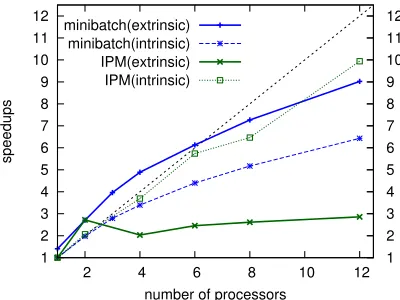
Figure 4 gives a detailed analysis of speedups. Here we perform both extrinsic and intrinsic com-parisons. In the former, we care about the time to reach a given accuracy; in this plot we use 92.27 which is the converged accuracy of IPM on 12 pro-cessors. We choose it since it is the lowest

1 2 3 4 5 6 7 8 9 10 11 12

2 4 6 8 10 12 1 2 3 4 5 6 7 8 9 10 11 12

speedups

number of processors minibatch(extrinsic)

minibatch(intrinsic) IPM(extrinsic) IPM(intrinsic)

Figure 4: Speedups of minibatch parallelization vs. IPM on 1 to 12 processors (parsing with MIRA). Extrinsic comparisons use “the time to reach an accuracy of 92.27” for speed calculations, 92.27 being the converged accu-racy of IPM using 12 processors. Intrinsic comparisons use average time per iteration regardless of accuracy.

racy among all converged models; choosing a higher accuracy would reveal even larger speedups for our methods. This figure shows that our method offers superlinear speedups with small number of proces-sors (1 to 6), and almost linear speedups with large number of processors (8 and 12). Note that even

p= 1offers a speedup of 1.5 thanks to serial mini-batch’s faster convergence; in other words, within the 9 fold speed-up atp = 12, parallelization con-tributes about6 and minibatch about1.5. By con-trast, IPM only offers an almost constant speedup of around 3, which is consistent with the findings of McDonald et al. (2010) (both of their experiments show a speedup of around 3).

We also try to understand where the speedup comes from. For that purpose we study intrinsic speedup, which is about the speed regardless of ac-curacy (see Figure 4). For our minibatch method, intrinsic speedup is the average time per iteration of a parallel run over the serial minibatch base-line. This answers the questions such as “how CPU-efficient is our parallelization” or “how much CPU time is wasted”. We can see that with small num-ber of processors (2 to 4), theefficiency, defined as

96.8 96.85 96.9 96.95 97 97.05

0 0.2 0.4 0.6 0.8 1 1.2 1.4 1.6 1.8

accuracy on held-out

wall-clock time (hours) m=1 m=16 m=24 m=48

Figure 5: Minibatch learning for tagging with perceptron (m = 16,24,32) compared with baseline (m = 1) for tagging with perceptron. All curves are on single CPU.

wasted. This wasting is due to two sources: first, the load-balancing problem worsens with more proces-sors, and secondly, the update procedure still runs in serial mode withp−1processors sleeping.

5.2 Part-of-Speech Tagging with Perceptron

Part-of-speech tagging is usually considered as a simpler task compared to dependency parsing. Here we show that using minibatch can also bring better accuracies and speedups for part-of-speech tagging. We implement a part-of-speech tagger with aver-aged perceptron. Following the standard splitting of Penn Treebank (Collins, 2002), we use Sections 00-18 for training and Sections 19-21 as held-out. Our implementation provides an accuracy of96.98with beam size8.

First we run the tagger on a single processor with minibatch sizes 8, 16, 24, and 32. As in Figure 5, we observe similar convergence acceleration and higher accuracies with minibatch. In particular, minibatch of size m = 16 provides the highest accuracy of 97.04, giving an improvement of 0.06. This im-provement is smaller than what we observe in MIRA learning for dependency parsing experiments, which can be partly explained by the fast convergence of the tagger, and that perceptron does not involve op-timization in the updates.

Then we choose minibatch of size 24 to investi-gate the parallelization performance. As Figure 6 (top) shows, with 12 processors our method takes only0.10hours to converge to an accuracy of97.00, compared to the baseline of96.98 with0.45 hours. We also compare our method with IPM as in

96.8 96.85 96.9 96.95 97

0 0.2 0.4 0.6 0.8 1 1.2 1.4 1.6 1.8

accuracy

baseline m=24,p=1 m=24,p=4 m=24,p=12

96.8 96.85 96.9 96.95 97

0 0.2 0.4 0.6 0.8 1 1.2 1.4 1.6 1.8

accuracy

wall-clock time (hours) baseline IPM,p=4 IPM,p=12

Figure 6: Parallelized minibatch is faster than iterative parameter mixing (on tagging with perceptron). Top: minibatch of size 24 using 4 and 12 processors offers significant speedups over the baselines. Bottom: IPM with the same4and12processors offers slightly smaller speedups. Note that IPM with 4 processors converges lower than other parallelization curves.

ure 6 (bottom). Again, our method converges faster and better than IPM, but this time the differences are much smaller than those in parsing.

Figure 7 uses 96.97 as a criteria to evaluate the extrinsic speedups given by our method and IPM. Again we choose this number because it is the lowest accuracy all learners can reach. As the figure sug-gests, although our method does not have a higher pure parallelization speedup (intrinsic speedup), it still outperforms IPM.

1 2 3 4 5 6 7 8 9 10 11 12

2 4 6 8 10 12 1 2 3 4 5 6 7 8 9 10 11 12

speedup ratio

number of processors minibatch(extrinsic)

minibatch(intrinsic) IPM(extrinsic) IPM(intrinsic)

Figure 7: Speedups of minibatch parallelization and IPM on1to12processors (tagging with perceptron). Extrin-sic speedup uses “the time to reach an accuracy of96.97” as the criterion to measure speed. Intrinsic speedup mea-sures the pure parallelization speedup. IPM has an al-most linear intrinsic speedup but a near constant extrinsic speedup of about 3 to 4.

0 10 20 30 40 50 60

2 4 6 8 10 12

% of waiting time

number of processors parser(balanced)

tagger(balanced) parser(unbalanced) tagger(unbalanced)

Figure 8: Percentage of time wasted due to synchroniza-tion (waiting for other processors to finish) (minibatch m = 24), which corresponds to the gray blocks in Fig-ure 1 (b-c). The number of sentences assigned to each processor decreases with more processors, which wors-ens the unbalance. Our load-balancing strategy (Figure 1 (c)) alleviates this problem effectively. The communica-tion overhead and update time arenotincluded.

6 Related Work and Discussions

Besides synchronous minibatch and iterative param-eter mixing (IPM) discussed above, there is another method of asychronous minibatch parallelization (Zinkevich et al., 2009; Gimpel et al., 2010; Chiang, 2012), as in Figure 1. The key advantage of asyn-chronous over synasyn-chronous minibatch is that the for-mer allows processors to remain near-constant use,

while the latter wastes a significant amount of time when some processors finish earlier than others in a minibatch, as found in our experiments. Gimpel et al. (2010) show significant speedups of asychronous parallelization over synchronous minibatch on SGD and EM methods, and Chiang (2012) finds asyn-chronous parallelization to be much faster than IPM on MIRA for machine translation. However, asyn-chronous is significantly more complicated to imple-ment, which involves locking when one processor makes an update (see Fig. 1 (d)), and (in languages like Python) message-passing to other processors af-ter update. Whether this added complexity is worth-while on large-margin learning is an open question.

7 Conclusions and Future Work

We have presented a simple minibatch paralleliza-tion paradigm to speed up large-margin structured learning algorithms such as (averaged) perceptron and MIRA. Minibatch has an advantage in both se-rial and parallel settings, and our experiments con-firmed that a minibatch size of around 16 or 24 leads to a significant speedups over the pure online base-line, and when combined with parallelization, leads to almost linear speedups for MIRA, and very signif-icant speedups for perceptron. These speedups are significantly higher than those of iterative parame-ter mixing of McDonald et al. (2010) which were almost constant (3∼4) in both our and their own ex-periments regardless of the number of processors.

One of the limitations of this work is that although decoding is done in parallel, update is still done in serial and in MIRA the quadratic optimization step (Hildreth algorithm (Hildreth, 1957)) scales super-linearly with the number of constraints. This pre-vents us from using very large minibatches. For future work, we would like to explore parallelized quadratic optimization and larger minibatch sizes, and eventually apply it to machine translation.

Acknowledgement

References

David Chiang. 2012. Hope and fear for discriminative training of statistical translation models. J. Machine Learning Research (JMLR), 13:1159–1187.

C.-T. Chu, S.-K. Kim, Y.-A. Lin, Y.-Y. Yu, G. Bradski, A. Ng, and K. Olukotun. 2007. Map-reduce for ma-chine learning on multicore. In Advances in Neural Information Processing Systems 19.

Michael Collins and Brian Roark. 2004. Incremental parsing with the perceptron algorithm. InProceedings of ACL.

Michael Collins. 2002. Discriminative training meth-ods for hidden markov models: Theory and experi-ments with perceptron algorithms. InProceedings of EMNLP.

Koby Crammer and Yoram Singer. 2003. Ultraconser-vative online algorithms for multiclass problems. J. Mach. Learn. Res., 3:951–991, March.

Jenny Rose Finkel, Alex Kleeman, and Christopher D. Manning. 2008. Efficient, feature-based, conditional random field parsing. InProceedings of ACL.

Kevin Gimpel, Dipanjan Das, and Noah Smith. 2010. Distributed asynchronous online learning for natural language processing. InProceedings of CoNLL. Clifford Hildreth. 1957. A quadratic programming

pro-cedure. Naval Research Logistics Quarterly, 4(1):79– 85.

Liang Huang and Kenji Sagae. 2010. Dynamic program-ming for linear-time incremental parsing. In Proceed-ings of ACL 2010.

Liang Huang, Suphan Fayong, and Yang Guo. 2012. Structured perceptron with inexact search. In Proceed-ings of NAACL.

John Lafferty, Andrew McCallum, and Fernando Pereira. 2001. Conditional random fields: Probabilistic mod-els for segmenting and labeling sequence data. In Pro-ceedings of ICML.

Percy Liang and Dan Klein. 2009. Online em for unsu-pervised models. InProceedings of NAACL.

Ryan McDonald and Fernando Pereira. 2006. On-line learning of approximate dependency parsing al-gorithms. InProceedings of EACL.

Ryan McDonald, Koby Crammer, and Fernando Pereira. 2005. Online large-margin training of dependency parsers. InProceedings of the 43rd ACL.

Ryan McDonald, Keith Hall, and Gideon Mann. 2010. Distributed training strategies for the structured per-ceptron. InProceedings of NAACL, June.

Shai Shalev-Shwartz, Yoram Singer, and Nathan Srebro. 2007. Pegasos: Primal estimated sub-gradient solver for svm. InProceedings of ICML.