Weakly Supervised Natural Language Learning Without Redundant Views

Weakly Supervised Natural Language Learning Without Redundant Views

Vincent Ng and Claire Cardie

Department of Computer Science

Cornell University

Ithaca, NY 14853-7501

yung,cardie

@cs.cornell.edu

Abstract

We investigate single-view algorithms as an al-ternative to multi-view algorithms for weakly supervised learning for natural language pro-cessing tasks without a natural feature split. In particular, we apply co-training, self-training, and EM to one such task and find that both self-training and FS-EM, a new variation of EM that incorporates feature selection, outperform co-training and are comparatively less sensitive to parameter changes.

1

Introduction

Multi-view weakly supervised learning paradigms such as co-training (Blum and Mitchell, 1998) and co-EM (Nigam and Ghani, 2000) learn a classification task from a small set of labeled data and a large pool of unla-beled data using separate, but redundant, views of the data (i.e. using disjoint feature subsets to represent the

data). Multi-view learning has been successfully

ap-plied to a number of tasks in natural language processing (NLP), including text classification (Blum and Mitchell, 1998; Nigam and Ghani, 2000), named entity classifica-tion (Collins and Singer, 1999), base noun phrase brack-eting (Pierce and Cardie, 2001), and statistical parsing (Sarkar, 2001; Steedman et al., 2003).

The theoretical performance guarantees of multi-view weakly supervised algorithms come with two fairly strong assumptions on the views. First, each view must be sufficient to learn the given concept. Second, the views must be conditionally independent of each other given the class label. When both conditions are met, Blum and Mitchell prove that an initial weak learner can be boosted using unlabeled data.

Unfortunately, finding a set of views that satisfies both of these conditions is by no means an easy problem. In addition, recent empirical results by Muslea et al. (2002)

and Nigam and Ghani (2000) have shown that multi-view algorithms are quite sensitive to the two underlying as-sumptions on the views. Effective view factorization in multi-view learning paradigms, therefore, remains an im-portant issue for their successful application. In practice, views are supplied by users or domain experts, who deter-mine a natural feature split that is expected to be redun-dant (i.e. each view is expected to be sufficient to learn the target concept) and conditionally independent given

the class label.1

We investigate here the application of weakly super-vised learning algorithms to problems for which no obvi-ous natural feature split exists and hypothesize that, in these cases, single-view weakly supervised algorithms will perform better than their multi-view counterparts. Motivated, in part, by the results in Mueller et al. (2002), we use the task of noun phrase coreference resolution

for illustration throughout the paper.2 In our

experi-ments, we compare the performance of the Blum and Mitchell co-training algorithm with that of two com-monly used single-view algorithms, namely, self-training and Expectation-Maximization (EM). In comparison to co-training, self-training achieves substantially superior performance and is less sensitive to its input parameters. EM, on the other hand, fails to boost performance, and we attribute this phenomenon to the presence of redun-dant features in the underlying generative model. Con-sequently, we propose a wrapper-based feature selection method (John et al., 1994) for EM that results in perfor-mance improvements comparable to that observed with self-training. Overall, our results suggest that single-view

1

Abney (2002) argues that the conditional independence as-sumption is remarkably strong and is rarely satisfied in real data sets, showing that a weaker independence assumption suffices.

2

Mueller et al. (2002) explore a heuristic method for view factorization for the related problem of anaphora resolution, but find that co-training shows no performance improvements for any type of German anaphor except pronouns over a baseline classifier trained on a small set of labeled data.

weakly supervised learning algorithms are a viable al-ternative to multi-view algorithms for data sets where a natural feature split into separate, redundant views is not available.

The remainder of the paper is organized as follows. Section 2 presents an overview of the three weakly su-pervised learning algorithms mentioned previously. In section 3, we introduce noun phrase coreference resolu-tion and describe the machine learning framework for the problem. In section 4, we evaluate the weakly supervised learning algorithms on the task of coreference resolution. Section 5 introduces a method for improving the perfor-mance of weakly supervised EM via feature selection. We conclude with future work in section 6.

2

Weakly Supervised Algorithms

In this section, we give a high-level description of our im-plementation of the three weakly supervised algorithms that we use in our comparison, namely, co-training, self-training, and EM.

2.1 Co-Training

Co-training (Blum and Mitchell, 1998) is a multi-view weakly supervised algorithm that trains two classifiers that can help augment each other’s labeled data using two separate but redundant views of the data. Each classifier is trained using one view of the data and predicts the la-bels for all instances in the data pool, which consists of a randomly chosen subset of the unlabeled data. Each then selects its most confident predictions from the pool and adds the corresponding instances with their predicted labels to the labeled data while maintaining the class dis-tribution in the labeled data.

The number of instances to be added to the labeled data by each classifier at each iteration is limited by a pre-specified growth size to ensure that only the instances that have a high probability of being assigned the correct label are incorporated. The data pool is refilled with in-stances drawn from the unlabeled data and the process is repeated for several iterations. During testing, each clas-sifier makes an independent decision for a test instance and the decision associated with the higher confidence is taken to be the final prediction for the instance.

2.2 Self-Training

Self-training is a single-view weakly supervised algo-rithm that has appeared in various forms in the literature. The version of the algorithm that we consider here is a variation of the one presented in Banko and Brill (2001). Initially, we use bagging (Breiman, 1996) to train a committee of classifiers using the labeled data. Specifi-cally, each classifier is trained on a bootstrap sample cre-ated by randomly sampling instances with replacement

from the labeled data until the size of the bootstrap sam-ple is equal to that of the labeled data. Then each member of the committee (or bag) predicts the labels of all unla-beled data. The algorithm selects an unlaunla-beled instance for adding to the labeled data if and only if all bags agree upon its label. This ensures that only the unlabeled in-stances that have a high probability of being assigned the correct label will be incorporated into the labeled set. The above steps are repeated until all unlabeled data is labeled or a fixed point is reached. Following Breiman (1996), we perform simple majority voting using the committee to predict the label of a test instance.

2.3 EM

The use of EM as a single-view weakly supervised clas-sification algorithm is introduced in Nigam et al. (2000). Like the classic unsupervised EM algorithm (Dempster et al., 1977), weakly supervised EM assumes a paramet-ric model of data generation. The labels of the unlabeled data are treated as missing data. The goal is to find a model such that the posterior probability of its parame-ters is locally maximized given both the labeled data and the unlabeled data.

Initially, the algorithm estimates the model parame-ters by training a probabilistic classifier on the labeled instances. Then, in the E-step, all unlabeled data is prob-abilistically labeled by the classifier. In the M-step, the parameters of the generative model are re-estimated us-ing both the initially labeled data and the probabilistically labeled data to obtain a maximum a posteriori (MAP) hy-pothesis. The E-step and the M-step are repeated for sev-eral iterations. The resulting model is then used to make predictions for the test instances.

3

The Machine Learning Framework for

Coreference Resolution

Noun phrase coreference resolution refers to the problem of determining which noun phrases (NPs) refer to each real-world entity mentioned in a document. In this sec-tion, we give an overview of the coreference resolution system to which the weakly supervised algorithms de-scribed in the previous section are applied.

The framework underlying the system is a standard combination of classification and clustering employed by supervised learning approaches (e.g. Ng and Cardie (2002); Soon et al. (2001)). Specifically, coreference res-olution is recast as a classification task, in which a pair of NPs is classified as co-referring or not based on con-straints that are learned from an annotated corpus. Train-ing instances are generated by pairTrain-ing each NP with each of its preceding NPs in the document. The classification

associated with a training instance is one of COREFER

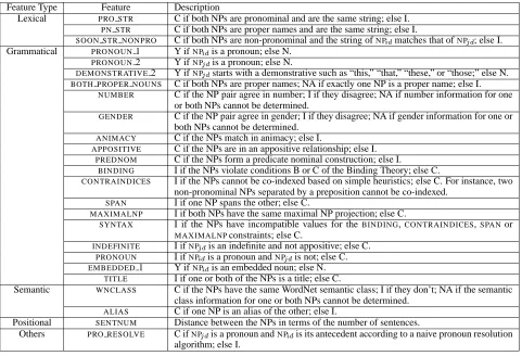
Feature Type Feature Description

Lexical PRO STR C if both NPs are pronominal and are the same string; else I.

PN STR C if both NPs are proper names and are the same string; else I.

SOON STR NONPRO C if both NPs are non-pronominal and the string ofNP matches that ofNP; else I.

Grammatical PRONOUN1 Y ifNP is a pronoun; else N.

PRONOUN2 Y ifNP is a pronoun; else N.

DEMONSTRATIVE2 Y ifNP starts with a demonstrative such as “this,” “that,” “these,” or “those;” else N.

BOTH PROPER NOUNS C if both NPs are proper names; NA if exactly one NP is a proper name; else I.

NUMBER C if the NP pair agree in number; I if they disagree; NA if number information for one or both NPs cannot be determined.

GENDER C if the NP pair agree in gender; I if they disagree; NA if gender information for one or both NPs cannot be determined.

ANIMACY C if the NPs match in animacy; else I.

APPOSITIVE C if the NPs are in an appositive relationship; else I.

PREDNOM C if the NPs form a predicate nominal construction; else I.

BINDING I if the NPs violate conditions B or C of the Binding Theory; else C.

CONTRAINDICES I if the NPs cannot be co-indexed based on simple heuristics; else C. For instance, two non-pronominal NPs separated by a preposition cannot be co-indexed.

SPAN I if one NP spans the other; else C.

MAXIMALNP I if both NPs have the same maximal NP projection; else C.

SYNTAX I if the NPs have incompatible values for theBINDING,CONTRAINDICES,SPANor

MAXIMALNPconstraints; else C.

INDEFINITE I ifNP is an indefinite and not appositive; else C.

PRONOUN I ifNP is a pronoun andNP is not; else C.

EMBEDDED1 Y ifNP is an embedded noun; else N.

TITLE I if one or both of the NPs is a title; else C.

Semantic WNCLASS C if the NPs have the same WordNet semantic class; I if they don’t; NA if the semantic class information for one or both NPs cannot be determined.

ALIAS C if one NP is an alias of the other; else I.

Positional SENTNUM Distance between the NPs in terms of the number of sentences.

Others PRO RESOLVE C ifNP is a pronoun andNP is its antecedent according to a naive pronoun resolution

algorithm; else I.

Table 1: Feature set for the coreference system.The feature set contains relational and non-relational features that are used to

generate an instance representing two NPs,NP andNP, in document , whereNP precedesNP. Non-relational features test

some property P of one of the NPs under consideration and take on a value of YESor NOdepending on whether P holds. Relational features test whether some property P holds for the NP pair under consideration and indicate whether the NPs are COMPATIBLEor

INCOMPATIBLEw.r.t. P; a value of NOTAPPLICABLEis used when property P does not apply.

co-refer in the text. A separate clustering mechanism then coordinates the possibly contradictory pairwise classifi-cations and constructs a partition on the set of NPs.

We perform the experiments in this paper

using our coreference resolution system (see

Ng and Cardie (2002)). For the sake of

complete-ness, we include the descriptions of the 25 features

employed by the system in Table 1. Linguistically,

the features can be divided into five groups: lexical, grammatical, semantic, positional, and others. However, we use naive Bayes rather than decision tree induction as the underlying learning algorithm to train a coreference classifier, simply because (1) it provides a generative model assumed by EM and hence facilitates comparison between different approaches and (2) it is more robust to the skewed class distributions inherent in coreference data sets than decision tree learners. When the corefer-ence system is used within the weakly supervised setting, a weakly supervised algorithm bootstraps the

corefer-ence classifier from the given labeled and unlabeled data rather than from a much larger set of labeled instances.

We conclude this section by noting that view factor-ization is a non-trivial task for coreference resolution. For many lexical tagging problems such as part-of-speech tagging, views can be drawn naturally from the left-hand and right-hand context. For other tasks such as named en-tity classification, views can be derived from features in-side and outin-side the phrase under conin-sideration (Collins and Singer, 1999). Unfortunately, neither of these op-tions is possible for coreference resolution. We will ex-plore several heuristic methods for view factorization in the next section.

4

Evaluation

4.1 Experimental Setup

To ensure a fair comparison of the weakly supervised algorithms, the experiments are designed to determine the best parameter setting of each algorithm (in terms of its effectiveness to improve performance) for the data sets we investigate. Specifically, we keep the parame-ters common to all three weakly supervised algorithms (i.e. the labeled and unlabeled data) constant and vary the algorithm-specific parameters, as described below.

Evaluation. We use the MUC-6 (1995) and MUC-7 (1998) coreference data sets for evaluation. The training set is composed of 30 “dry run” texts, 1 of which is se-lected to be the annotated text and the remaining 29 texts are used as unannotated data. For MUC-6, 3486 training instances are generated from 84 NPs in the annotated text. For MUC-7, 3741 training instances are generated from 87 NPs. The unlabeled data is composed of 488173 in-stances and 478384 inin-stances for the MUC-6 and MUC-7 data sets, respectively. Testing is performed by applying the bootstrapped coreference classifier and the clustering algorithm described in section 3 on the 20–30 “formal evaluation” texts for each of the MUC-6 and MUC-7 data sets.

Co-training parameters. The co-training parameters are set as follows.

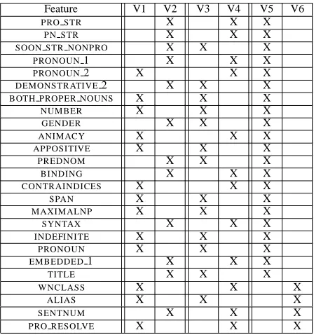
Views. We tested three pairs of views. Table 2

re-produces the 25 features of the coreference system and shows the views we employ. Specifically, the three view pairs are generated by the following methods.

Mueller et al.’s heuristic method. Starting from two empty views, the iterative algorithm selects for each view the feature whose addition maximizes the per-formance of the respective view on the labeled data

at each iteration. 3 _{This method produces the view}

pair V1 and V2 in Table 2 for the MUC-6 data set. A different view pair is produced for MUC-7.

Random splitting of features into views. Starting from two empty views, an iterative algorithm that randomly chooses a feature for each view at each step is used to split the feature set. The resulting view pair V3 and V4 is used for both the MUC-6 and MUC-7 data sets.

Splitting of features according to the feature type. Specifically, one view comprises the lexico-syntactic features and the other the remaining ones. This approach produces the view pair V5 and V6, which is used for both data sets.

Pool size. We tested pool sizes of 500, 1000, 5000. Growth size. We tested values of 10, 50, 100, 200, 250.

3

Space limitation precludes a detailed description of this method. See Mueller et al. (2002) for details.

Feature V1 V2 V3 V4 V5 V6

PRO STR X X X

PN STR X X X

SOON STR NONPRO X X X

PRONOUN1 X X X

PRONOUN2 X X X

DEMONSTRATIVE2 X X X

BOTH PROPER NOUNS X X X

NUMBER X X X

GENDER X X X

ANIMACY X X X

APPOSITIVE X X X

PREDNOM X X X

BINDING X X X

CONTRAINDICES X X X

SPAN X X X

MAXIMALNP X X X

SYNTAX X X X

INDEFINITE X X X

PRONOUN X X X

EMBEDDED1 X X X

TITLE X X X

WNCLASS X X X

ALIAS X X X

SENTNUM X X X

PRO RESOLVE X X X

Table 2: Co-training view pairs employed by the

corefer-ence system.Column 1 lists the 25 features shown in Table 1.

Columns 2-7 show three different pairs of views that we have attempted for co-training coreference classifiers.

Number of co-training iterations. We monitored

per-formance on the test data at every 10 iterations of co-training and ran the algorithm until performance stabi-lized.

Self-training parameters. Given the labeled and unla-beled data, self-training requires only the specification of the number of bags. We tested all odd number of bags between 1 and 25.

EM parameters. Given the labeled and unlabeled data, EM has only one parameter — the number of iterations. We ran EM to convergence and kept track of its test set performance at every iteration.

4.2 Results and Discussion

Results are shown in Table 3, where performance is re-ported in terms of recall, precision, and F-measure using the model-theoretic MUC scoring program (Vilain et al., 1995). The baseline coreference system, which is trained only on the labeled document using naive Bayes, achieves an F-measure of 55.5 and 43.8 on the 6 and MUC-7 data sets, respectively.

Experiments MUC-6 MUC-7

Best Parameter Setting R P F Best Parameter Setting R P F

Baseline — 58.3 52.9 55.5 — 52.8 37.4 43.8

Co-Training v=V5/V6,g=50,p=5000,i=220 47.5 81.9 60.1 v=V5/V6,g=100,p=500,i=260 40.6 77.6 53.3

Self-Training b=7 54.1 78.6 64.1 b=9 54.6 62.6 58.3

EM i=20 64.8 51.8 57.6 i=2 54.1 40.7 46.4

FS-EM — 64.2 66.6 65.4 — 53.3 70.3 60.5

Table 3: Comparative results of co-training, self-training, EM, and FS-EM (to be described in section 5). Recall,

Precision, and F-measure are provided. For co-training, self-training, and EM, the best results (F-measure) achieved by the

algo-rithms and the corresponding parameter settings (with views v, growth size g, pool size p, number of iterations i, and number of bags b) are shown.

0 100 200 300 400 500 600 700 800 900 1000 30

40 50 60 70 80 90 100

Number of Co−Training Iterations

Score

Baseline Recall Precision F−measure

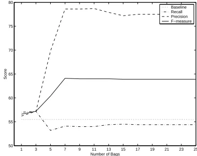
Figure 1: Learning curve for co-training (pool size = 5000, growth size = 50) for the MUC-6 data set.

results are obtained are also shown in the table. To get a better picture of the behavior of co-training, we present the learning curve for the co-training run that gives rise to the best F-measure for the MUC-6 data set in Figure 1. The horizontal (dotted) line shows the performance of the baseline system, which achieves an F-measure of 55.5, as described above. As co-training progresses, F-measure peaks at iteration 220 and then gradually drops below that of the baseline after iteration 570.

Although co-training produces substantial improve-ments over the baseline at its best parameter settings, a closer examination of our results reveals that they cor-roborate previous findings: the algorithm is sensitive not only to the number of iterations, but to other input pa-rameters such as the pool size and the growth size as well (Nigam and Ghani, 2000; Pierce and Cardie, 2001). The lack of a principled method for determining these param-eters in a weakly supervised setting where labeled data is scarce remains a serious disadvantage for co-training.

Self-training results are shown in row 3 of Table 3: self-training performs substantially better than both the baseline and co-training for both data sets. In contrast to co-training, however, self-training is relatively

insensi-1 3 5 7 9 11 13 15 17 19 21 23 25 50

55 60 65 70 75 80

Number of Bags

Score

Baseline Recall Precision F−measure

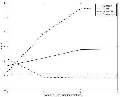
Figure 2: Effect of the number of bags on the perfor-mance of self-training for the MUC-6 data set.

tive to its input parameter. Figure 2 shows the fairly con-sistent performance of self-training with seven or more bags for the MUC-6 data set. We observe similar trends for the MUC-7 data set. These results are consistent with empirical studies of bagging across a variety of classifi-cation tasks where seven to 25 bags are deemed sufficient (Breiman, 1996).

0 1 2 3 50

55 60 65 70 75 80

Number of Self−Training Iterations

Score

Baseline Recall Precision F−measure

Figure 3: Learning curve for self-training using 7 bags for the MUC-6 data set.

the labeled data, thereby ensuring that precision will

in-crease.4

As we can see from Table 3, the recall level achieved by co-training is much lower than that of self-training. This is an indication that each co-training view is insuf-ficient to learn the concept: the feature split limits any interaction of features in different views that might pro-duce better recall. Overall, these results provide evidence that self-training is a better alternative to co-training for weakly supervised learning for problems such as corefer-ence resolution where no natural feature split exists.

On the other hand, EM only gives rise to modest per-formance gains over the baseline system, as we can see from row 4 of Table 3. The performance of EM depends in part on the correctness of the underlying generative model (Nigam et al., 2000), which in our case is naive

Bayes. In this model, an instance with feature values

, ,

and class is created by first choosing

the class with prior probability and then

generat-ing each available feature

with probability

"!

independently, under the assumption that the feature val-ues are conditionally independent given the class. As a result, model correctness is adversely affected by redun-dant features, which clearly invalidate the conditional in-dependence assumption. In fact, naive Bayes is known to be bad at handling redundant features (Langley and Sage, 1994).

We hypothesize that the presence of redundant

fea-4_{When tackling the task of confusion set disambiguation,} Banko and Brill (2001) observe only modest gains from self-training by bootstrapping from a seed corpus of one million words. We speculate that a labeled data set of this size can possibly enable them to train a reasonably good classifier with which self-training can only offer marginal benefits, but the re-lationship between the behavior of self-training and the size of the seed (labeled) corpus remains to be shown.

tures causes the generative model and hence EM to per-form poorly. Although self-training depends on the same model, it only makes use of the binary decisions returned by the model and is therefore more robust to the naive Bayes assumptions, as reflected in its fairly impressive

empirical performance.5 In contrast, the fact that EM

re-lies on the probability estimates of the model makes it more sensitive to the correctness of the model.

5

Meta-Bootstrapping with Feature

Selection

If our hypothesis regarding the presence of redundant features were correct, then feature selection could re-sult in an improved generative model, which could in turn improve the performance of weakly supervised EM. This section discusses a wrapper-based feature selection method for EM.

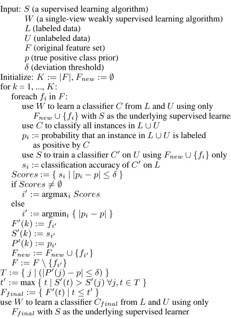
5.1 A Two-Tiered Bootstrapping Algorithm

We now describe the FS-EM algorithm for boosting the performance of weakly supervised algorithms via feature selection. Although named after EM, the algorithm as de-scribed is potentially applicable to all single-view weakly supervised algorithms. FS-EM takes as input a super-vised learner, a single-view weakly supersuper-vised learner, a

labeled data set# , and an unlabeled data set$ . In

addi-tion, it assumes knowledge of the positive class prior (i.e. the true percentage of positive instances in the data) like co-training and requires a deviation threshold that we will explain shortly.

FS-EM, which has a two-level bootstrapping structure, is reminiscent of the meta-bootstrapping algorithm intro-duced in Riloff and Jones (1999). The outer-level boot-strapping task is feature selection, whereas the inner-level task is to learn a bootstrapped classifier from labeled and unlabeled data as described in section 4. At a high level, FS-EM uses a forward feature selection algorithm to im-pose a total ordering on the features based on the order in which the features are selected. Specifically, FS-EM

per-forms the three steps below for each feature %'& that has

not been selected. First, it uses the weakly supervised

learner to train a classifier( from the labeled and

unla-beled data (#)$ ) using only the feature%'& as well as the

features selected thus far. Second, the algorithm uses(

to classify all of the instances in#*)+$ . Finally, FS-EM

trains a new model on just$ , which is now labeled by( .

At the end of the three steps, exactly one model is trained for each feature that has not been selected. The forward selection algorithm then selects the feature with which the corresponding model achieves the best performance

5

on# (w.r.t. the true labels of the instances in# ) for

addi-tion to,-/.0 (the set of features selected thus far).

6 _The

process is repeated until all features have been selected.

Unfortunately, since # can be small, selecting a

fea-ture for incorporation into , -1.20 by measuring the

per-formance of the corresponding model on # may not

ac-curately reflect the actual model performance. To han-dle this problem, FS-EM has a preference for adding fea-tures whose inclusion results in a classification in which the positive class prior (i.e. the probability that an

in-stance is labeled as positive),3 &, does not deviate from the

true positive class prior,3 , by more than a pre-specified

threshold value,4 . A large deviation from the true prior

is an indication that the resulting classification of the data does not correspond closely to the actual classification. This algorithmic bias is particularly useful for weakly su-pervised learners (such as EM) that optimize an objective function other than classification accuracy and can poten-tially produce a classification that is substanpoten-tially differ-ent from the actual one. Specifically, FS-EM attempts to ensure that the classification produced by the weakly supervised learner weakly agrees with the actual classi-fication, where the weak disagreement rate between two classifications is defined as the difference between their positive class priors. Note that weak agreement is a nec-essary but not sufficient condition for two classifications

to be identical.7

Nevertheless, if the addition of any of the features to

, -1.20 does not produce a classification that weakly agrees

with the true one, FS-EM picks the feature whose inclu-sion results in a positive class prior that has the least de-viation instead. This step can be viewed as introducing “pseudo-random” noise into the feature selection process. The hope is that the deviation of the high-scoring, “high-deviation” features can be lowered by first incorporating those with “low deviation”, thus continuing to strive for weak agreement while potentially achieving better

per-formance on# .

The final set of features, ,5&-16"7, is composed of the

first8 features chosen by the feature selection algorithm,

where8 is the largest number of features that can achieve

the best performance on # subject to the condition that

the corresponding classification produced by the weakly supervised algorithm weakly disagrees with the true one

by at most 4 . The output of FS-EM is a classifier that

the weakly supervised learner learns from# and$ using

only the features in, 5&-16"7. The pseudo-code describing

FS-EM is shown in Figure 4.

6

The reason for using only9 (instead of9 and : ) in the

validation step is primarily to preclude the possibility of get-ting a poor estimation of model performance as a result of the presence of potentially inaccurately labeled data from: .

7

In other words,;=<>;/ does not imply that the

correspond-ing classifications are identical.

Input:? (a supervised learning algorithm)

@

(a single-view weakly supervised learning algorithm)

9 (labeled data) : (unlabeled data)

A

(original feature set)

; (true positive class prior)

B (deviation threshold) Initialize:CEDF<HG A G, AJILKNM DF<PO

forQ = 1, ...,C :

foreachR' in

A

: use@

to learn a classifierS from9 and: using only AJITKNMUV

R'XW with? as the underlying supervised learner

useS to classify all instances in9

U

:

; := probability that an instance in9

U

: is labeled

as positive byS

use? to train a classifierSJY on: using A ILKNM UV

R

W only

Z

:= classification accuracy ofS Y on9 ?\[^]_"` Z DF< V Z aGTG;\\bc;dGTe B W if?\[f]_"` Zhg <iO j

Y DF< argmaxk?\[^]_"`

Z else j YlDF< argmin V G;\dbc;dGTW A Ynm Q1oDp<qR sr ? Ynm Q1o Dp< Z sr t Ynm

Q1oDp<i; r AJILKNM DF< AJILKNMUV R ur W A Dp< AwvxV

R urW

y DF< V z G m G t Ynm z o{b|;dG1e B oW } Y DF< max V } GT? Y m } o~? Y m z o€ zL‚}Jƒ y

W A„ IL…f† Dp< V A Ym } olG } e } YdW use@

to learn a classifierS

„

IL…f†

from9 and: using only A„

IT…f†

with? as the underlying supervised learner

returnS

„

IT…2†

Figure 4: The FS-EM algorithm.

5.2 Results and Discussion

We instantiate FS-EM with naive Bayes as the supervised learner and EM as the weakly supervised learner, provid-ing it with the same amount of labeled and unlabeled data

as in previous experiments and setting4 to 0.01. EM is

run for 7 iterations whenever it is invoked.8 _Results

us-ing FS-EM are shown in row 5 of Table 3. In comparison to EM, F-measure increases from 57.6 to 65.4 for MUC-6, and from 46.4 to 60.5 for MUC-7, allowing FS-EM to even surpass the performance of self-training. These results are consistent with our hypothesis that the perfor-mance of EM can be boosted by improving the underly-ing generative model usunderly-ing feature selection.

Finally, although FS-EM is only applicable to two-class problems, it can be generalized fairly easily to han-dle multi-class problems, where the true label distribution

8

is assumed to be available and the weak agreement rate can be measured based on the similarity of two distribu-tions.

6

Conclusions and Future Work

We have investigated single-view algorithms (self-training and EM) as an alternative to multi-view algo-rithms (co-training) for weakly supervised learning for problems that do not appear to have a natural feature split. Experimental results on two coreference data sets indi-cate that self-training outperforms co-training under vari-ous parameter settings and is comparatively less sensitive to parameter changes. While weakly supervised EM is not able to outperform co-training, we introduce a varia-tion of EM, FS-EM, for boosting the performance of EM via feature selection. Like self-training, FS-EM easily outperforms co-training.

Co-training algorithms such as CoBoost (Collins and Singer, 1999) and Greedy Agreement (Abney, 2002) that explicitly trade classifier agreement on unlabeled data against error on labeled data may be more robust to the underlying assumptions of co-training and can conceiv-ably perform better than the Blum and Mitchell algorithm

for problems without a natural feature split.9 _{Other less}

studied single-view weakly supervised algorithms in the NLP community such as co-training with different learn-ing algorithms (Goldman and Zhou, 2000) and graph mincuts (Blum and Chawla, 2001) can be similarly ap-plied to these problems to further test our original hy-pothesis. We plan to explore these possibilities in future research.

Acknowledgments

We thank Lillian Lee, Thorsten Joachims, and the Cor-nell NLP group including Regina Barzilay, Eric Breck, Bo Pang, and Steven Baker for many helpful comments. We also thank three anonymous reviewers for their feed-back and Ted Pedersen for encouraging us to apply en-semble methods to coreference resolution. This work was supported in part by NSF Grant IIS–0208028.

References

S. Abney. 2002. Bootstrapping. In Proceedings of the ACL, pages 360–367.

M. Banko and E. Brill. 2001. Scaling to very very large corpora for natural language disambiguation. In Proceedings of the

ACL/EACL, pages 26–33.

A. Blum and S. Chawla. 2001. Learning from labeled and un-labeled data using graph mincuts. In Proceedings of ICML, pages 19–26.

9

Indeed, Dasgupta et al. (2001) show that, when the condi-tional independence assumption of the views is satisfied, view classifiers whose agreement on unlabeled data is explicitly max-imized will have low generalization error.

A. Blum and T. Mitchell. 1998. Combining labeled and unla-beled data with co-training. In Proceedings of COLT, pages 92–100.

L. Breiman. 1996. Bagging predictors. Machine Learning, 24:123–140.

M. Collins and Y. Singer. 1999. Unsupervised models for named entity classification. In Proceedings of EMNLP/VLC, pages 100–110.

S. Dasgupta, M. Littman, and D. McAllester. 2001. PAC gen-eralization bounds for co-training. In Advances in NIPS.

A. Dempster, N. Laird, and D. Rubin. 1977. Maximum likeli-hood from incomplete data via the EM algorithm. Journal of

the Royal Statistical Society, Series B, 39(1):1–38.

P. Domingos and M. J. Pazzani. 1997. On the optimality of the simple Bayesian classifier under zero-one loss. Machine

Learning, 29:103–130.

S. Goldman and Y. Zhou. 2000. Enhancing supervised learning with unlabeled data. In Proceedings of ICML, pages 327– 334.

G. John, R. Kohavi, and K. Pfleger. 1994. Irrelevant features and the subset selection problem. In Proceedings of ICML.

P. Langley and S. Sage. 1994. Induction of selective Bayesian classifiers. In Proceedings of UAI, pages 399–406.

MUC-6. 1995. Proceedings of the Sixth Message

Understand-ing Conference (MUC-6).

MUC-7. 1998. Proceedings of the Seventh Message

Under-standing Conference (MUC-7).

C. Mueller, S. Rapp, and M. Strube. 2002. Applying co-training to reference resolution. In Proceedings of the ACL, pages 352–359.

I. Muslea, S. Minton, and C. Knoblock. 2002. Active + Semi-Supervised Learning = Robust Multi-View Learning. In

Pro-ceedings of ICML.

V. Ng and C. Cardie. 2002. Combining sample selection and error-driven pruning for machine learning of coreference rules. In Proceedings of EMNLP, pages 55–62.

K. Nigam and R. Ghani. 2000. Analyzing the effectiveness and applicability of co-training. In Proceedings of CIKM.

K. Nigam, A. McCallum, S. Thrun, and T. Mitchell. 2000. Text classification from labeled and unlabeled documents using EM. Machine Learning, 39(2/3):103–134.

D. Pierce and C. Cardie. 2001. Limitations of co-training for natural language learning from large datasets. In

Proceed-ings of EMNLP, pages 1–9.

E. Riloff and R. Jones. 1999. Learning dictionaries for infor-mation extraction by multi-level bootstrapping. In

Proceed-ings of AAAI, pages 474–479.

A. Sarkar. 2001. Applying co-training methods to statistical parsing. In Proceedings of the NAACL, pages 175–182.

W. M. Soon, H. T. Ng, and D. C. Y. Lim. 2001. A machine learning approach to coreference resolution of noun phrases.

Computational Linguistics, 27(4):521–544.

M. Steedman, M. Osborne, A. Sarkar, S. Clark, R. Hwa, J. Hockenmaier, P. Ruhlen, S. Baker, and J. Crim. 2003. Bootstrapping statistical parsers from small datasets. In

Pro-ceedings of the EACL.

M. Vilain, J. Burger, J. Aberdeen, D. Connolly, and L. Hirschman. 1995. A model-theoretic coreference scoring scheme. In Proceedings of the Sixth Message Understanding