Abstract — A MATLAB code has been developed based on REFPROP software for the design and analysis of Organic Rankine Cycle (ORC) systems. A small-scale ORC system using a scroll expander was designed using this code, and the effects of varying the expander pressure ratio, cycle maximum temperature, and presence of a recuperator were investigated. It was discovered that the fixed pressure ratio of a positive displacement device has a significant effect on the behaviour of the system although any losses incurred by not fully utilising the waste heat due to small expansion ratios can be mitigated by the use of a recuperator. The results will be presented and discussed in detail.
Index Terms—Organic Rankine Cycle, R245fa, Scroll Expander
I. INTRODUCTION
Energy efficiency and renewable energy are important and growing fields in engineering. The Organic Rankine Cycle is a promising technology that might allow energy to be extracted from untapped sources, or improve the efficiency of existing ones.
The Rankine Cycle using water as the working fluid is already widespread in power generation from nuclear and fossil fuels. However, below about 370°C, water becomes uneconomical as a working fluid [1]. This is partially because water has a high boiling point compared to many organic compounds, but also because water is a “wet” fluid, meaning that the right hand side of a T-S plot involving water has a negative slope. The implication of this is that, in order to avoid liquid droplets forming in the expander, the water must be superheated far above its boiling point. Fluids such as pentane and R245fa are “dry” fluids, meaning that the slope on the right hand side is non-negative, and saturated vapour can be expanded without condensation in the expander [2].
“Organic Rankine Cycle” is a catch-all term to describe a Rankine Cycle system using such working fluids, and is thermodynamically identical to conventional Rankine Cycle using water as working fluid. Possible applications for a low-temperature Organic Rankine Cycle system are many. Proposed uses include: Recovery of process heat from
This work is supported by Royal Society (RG130051)
Peter Collings is with the School of Engineering, University of Glasgow, Glasgow, Scotland, United Kingdom;
e-mail: [email protected]
* Corresponding author: Zhibin Yu is with the School of Engineering, University of Glasgow, Glasgow, Scotland, United Kingdom; E-mail:[email protected]
industry [3]; Solar Thermal electricity generation and desalination [4], [5]; Geothermal Energy [6] [7] and Biomass [8] [9], etc.
Higher power (>10kW) ORC systems are a relatively mature technology, and commercially available in the market. Little effort has been made to develop ORC system with a power output of less than 10 kW. However, due to energy price rises and strict legal restriction on carbon emission reductions, there will soon be a requirement for small ORC systems that can recover energy from relatively small scale waste heat sources, such as stationary diesel engines, heavy duty vehicles, or power generation locally using biomass combustion, etc. However, there are many challenges for developing such ORC systems with power levels less than 10 kW. The immediate difficulty is the lack of suitable expander. Turbines, screw expanders, and reciprocating piston expanders are not suitable for ORC systems with power level than 10 kW. Scroll expanders, and Rotary vane expanders can possibly be applied to low power applications. [10] However, there is lack of research in this area.
In this study, we aim to develop a lab-scale ORC system prototype using a scroll expander for future research. The power level is less than 1 kW, the heat source is hot water, and the heat sink is tap water. A computing code is firstly developed based on REFPROP, and then is validated against published experimental data. The validated code is then used to design our system. The design and analysis of this system will presented and discussed in detail in this paper.
II. CONCEPT DESIGN Temperature Range Selection
As this system will serve as an experimental rig for future research, so the temperature range was selected based on this. The highest hot water temperature analysed was 100°C, as this removed the need to pressurise the water to keep it a liquid, which is desirable for safety reasons, and the cold water temperature was chosen to be 15°C, as this was the temperature of the building tap water supply.
Expander Selection
The Organic Rankine Cycle system analysed in this paper is designed around a scroll expander. Such expander is a positive displacement device, which operates by rotating two spirals about each other, trapping and expanding fixed masses of vapour.
Scroll expanders are considered promising for low-power applications, as they are more efficient at these power levels than turbines as well as being cheaper, mechanically simpler, and a more mature technology for this sort of
Modelling and Analysis of a Small-Scale
Organic Rankine Cycle System with a Scroll
Expander
application [10] [11] [12]. It is therefore necessary to analyse their performance in ORC systems against other competing designs, such as screw and rotary vane expanders, in order to determine which is the most appropriate [13].
The model selected for our design is the AirSquared E15H22N425 1kW scroll expander. It has a pressure ratio of 3.5, although if a greater pressure ratio is desired, several can be connected in series.
Working Fluid Selection
The working fluid selected for this paper is R245fa. In theory, the MATLAB code developed for analysis can analyse any of a large list of fluids. R245fa was selected for a number of reasons. It has already been tested by Airsquared and found to be compatible with the expander. The other fluid tested, R123, is being phased out under the Monteal Protocol, and is therefore considered to have lesser potential for future development than R245fa. In addition, R245fa displays favourable performance over the selected temperature range, not requiring particularly high or low pressures to ensure it remains in the appropriate state at each stage of the cycle. R245fa has also already been used in a number of experimental papers operating under similar conditions to the ones considered below [1] [14] [15]. This means that results will be easier to validate.
III. MODELLING
A MATLAB model was built to analyse the Organic Rankine Cycle system linked to the REFPROP calculation software from the National Institute of Standards and Technology. The model worked around the system to calculate the properties at each point as follows:
The ratio of evaporator pressure to condenser pressure, the maximum temperature of the cycle, and the working fluid are defined by the user upon being prompted by the program.
In addition, the isentropic efficiency of the pump was taken to be 90%, and the expander to be 70%, as per the manufacturer’s specifications. The temperature of the cooling water in the condenser was set to be 15°C, as this was the measured temperature of the building cold water supply that will ultimately be used as a cooling source for any experimental rig. The minimum temperature of the working fluid was set to be 5°C above this. The power output at the shaft of the turbine was set to be 300W.
It was assumed that there was no energy transfer into or out of the system save that accounted for in the pump, evaporator, expander and condenser, and that there were no pressure drops in the heat exchangers or pipework. The states of the cycle were named as follows:
Initially, the cycle was analysed as if no recuperator was present, meaning state 2 was identical to state 3, and state 5 was identical to state 6 as shown in Fig. 1. And Fig 2.
[image:2.595.322.547.54.231.2]This is physically achieved by the use of bypass valves allowing the working fluid to circumvent the recuperator.
Fig. 1. Schematic of the Concept Design.
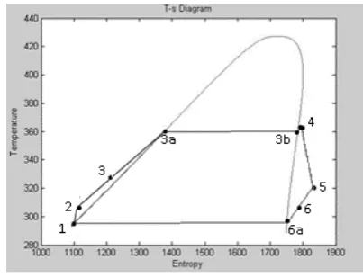
Fig. 2. Sample T-S diagram generated by the MATLAB model.
The temperature at the pump inlet (state 1) is already known, being the minimum temperature of the working fluid. The pressure is calculated as the minimum pressure required for the working fluid to remain a liquid at this temperature. REFPROP can then calculate the enthalpy and entropy under these conditions.
The pressure at the evaporator inlet (state 2) is determined by the ratio between the evaporator and condenser pressures. Multiplying the pressure at the pump inlet by this previously-defined ratio gives the pressure at the evaporator inlet. Assuming isentropic compression, S2,isentropic=S1. Knowing this, H3, isentropic can be calculated from REFPROP.
Finally, knowing H2, isentropic, H3 can be calculated using the equation:
,
(1) The remaining fluid properties at the evaporator inlet can now be calculated using REFPROP.
The temperature at the expander inlet (state 4) has already been defined by the user, and the pressure is the expander pressure, therefore the enthalpy and entropy can be calculated using REFPROP.
[image:2.595.329.531.268.422.2]condenser. Assuming isentropic expansion, S5,isentropic=S4. As before, H4, isentropic can be calculated from REFPROP, and H5 calculated using the equation:
, (2) The necessary mass flow rate of the working fluid to deliver a power output of 300W was calculated by dividing the required power output by the enthalpy difference across the expander:
′ (3) The model also featured the option of including a recuperator in the calculations. A recuperator is simply an additional heat exchanger in the cycle. The working fluid passes through the cold side of this heat exchanger between the pump and the evaporator, and the hot side between the expander and the condenser. This means that a certain proportion of the heat in the working fluid at the expander exit is used to preheat the working fluid before it enters the evaporator, reducing the heat demand of the evaporator.
The states at the exit of the recuperator were termed 3 for the cold side, and 6 for the hot side. The recuperator was modelled using an energy balance. It was assumed that no heat was lost to the surroundings, so any heat rejected by the hot side would be gained by the cold side.
The minimum temperature difference in the recuperator was set to 5°C. This point was located at the cold end, as the vapour phase has a lower specific heat capacity than the liquid phase.
This meant that T6 was equal to T2+5. Knowing the temperature and the pressure, the enthalpies of states 5 and 6 could be calculated. The enthalpy of state 3 could then be calculated by adding the enthalpy lost by the hot side to the enthalpy at the pump exit.
When the system was analysed without a recuperator, T3 was set to T2 and T6 to T5, effectively analysing the system with a recuperator of zero heat transfer area and length.
The heat source and sinks are assumed to be hot and cold water under atmospheric pressure, 101kPa. The flow rate of water through these is determined by the pinch point temperature difference.
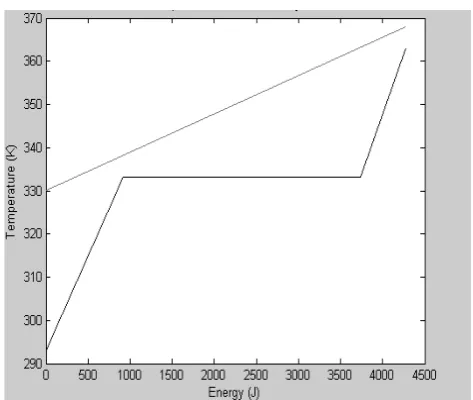
A graph of temperature against energy was produced for the working fluid and the heating water. The temperature difference at the hot water inlet and pinch point were set to be 5°C. This is consistent with the literature on the use of heat exchangers in Organic Rankine Cycles operating in a similar temperature range [16] [17] [18].
The total energy gained by the working fluid must be equal to the energy rejected by the water, assuming no energy loss to the environment.
Therefore, the temperature and energy transferred by the hot water is known at two points, the inlet and the pinch point. This allows a line to be drawn though these points and extrapolated to the hot water outlet.
This gives the hot water outlet temperature. Knowing the temperature difference and the energy transferred, the mass flow rate can be calculated using the equation:
[image:3.595.309.546.57.257.2], ∗ , ∗ ∆ (4)
Fig. 3: Plot of temperature against energy transferred. The upper line represents the hot water, the lower line the working fluid. The pinch point
can be clearly seen.
The First Law Efficiency is the ratio of net work out to heat energy in, and is given by:
(5)
The second law efficiency is given by a similar formula, with the Enthalpy H replaced by the Exergy I:
(6)
Exergy is given by the formula:
∗ (7)
Where the subscript 0 represents the ambient conditions of the system, in this case, the enthalpy and entropy the working fluid would have at the temperature and pressure of the cold water inlet (288K and 101kPa) [19]. These values can be pulled from REFPROP.
The second law efficiency is a measure of how well the cycle performs compared to an ideal cycle operating under the same conditions, and can be a more useful analysis tool than first law efficiency in some circumstances.
The waste heat utilisation factor was defined by the authors as the proportion of available energy (exergy) at the hot water inlet that was converted into useful work at the shaft of the expander, and was given by:
Table 1 : Comparison of experimental data and results from the model.
Table 2 : Parameters of the designed experimental rig
IV. RESULTS
The model was used to generate predictions of the performance of the system under a variety of operating conditions. The validation of the model as shown in Table 2 offers us the confidence to use this code to design analyse our prototype.
The maximum temperature of the cycle was set to be 5°C below the temperature of the hot water source. This allows the effect of the quality of the heat source to be determined. The pressure ratio of the cycle, when positive displacement devices such as a scroll expander are being used, represents the number of expanders strung together in series. For continuity of results, several intermediate pressures were analysed, even though only integer exponentials of 3.5 would be practically achievable using the AirSquared expander considered.
The recuperator scavenges heat from the condenser to preheat the working fluid after the pump. The effect that changing these parameters had on the first and second law efficiencies, and the waste heat utilisation factor was analysed.
[image:4.595.304.551.309.476.2]A Effect of Maximum Temperature
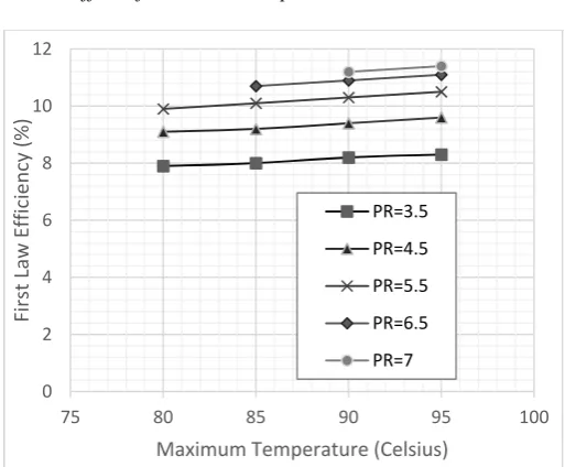
Fig. 4: Variation of First Law Efficiency with Maximum Temperature (with recuperator). PR denotes expander pressure ratio.
[image:4.595.42.284.354.527.2]Fig. 5 : Variation of First Law Efficiency with Maximum Temperature (without recuperator) . PR denotes expander pressure ratio.
Fig. 4 shows the relationship between the calculated efficiency and maximum heat source temperature for several different evaporation pressures when recuperator is used. As shown in Fig. 4, with a recuperator included in the model, the first law efficiency climbs with increasing maximum temperature. This is exactly as expected, as the Carnot efficiency increases with increasing maximum temperature.
However, interestingly, as shown in Fig. 5, when the recuperator is not included, the first law efficiency remains relatively constant. This is possibly because of the nature of the expander used. The scroll expander is a fixed displacement device, and it is constrained to operate at a constant pressure ratio. This means that the working fluid is not able to fully expand and reject all of its enthalpy as it passes through the expander. This means that a larger proportion of the heat is rejected in the condenser. With a recuperator, this is compensated for by the fact that a large proportion of this heat is recovered and used to pre-heat the fluid. Without a recuperator, this heat is lost from the system, and so the expected rise in efficiency is not observed.
0 2 4 6 8 10 12
75 80 85 90 95 100
First
Law
Efficiency
(%)
Maximum Temperature (Celsius)
PR=3.5
PR=4.5
PR=5.5
PR=6.5
PR=7
0 2 4 6 8 10 12
75 80 85 90 95 100
First
Law
Efficiency
(%)
Maximum Temperature (Celsius)
PR=3.5 PR=4.5 PR=5.5 PR=6.5 PR=7
Point Model Kang Difference
1 (Pump inlet)
T (K) 303 303 0 0.00% P (bar) 1.78 1.78 0 0.00% H (kJ/kg) 239.1 239 -0.1 -0.04% S (kJ/kg K) 1.135 1.14 0.005 0.40%
3a (saturated liquid)
T (K) 350.6 350 -0.556 -0.16% P (bar) 7.32 7.32 0 0.00% H (kJ/kg) 305.4 305 -0.4 -0.13% S (kJ/kg K) 1.337 1.34 0.003 0.22%
3b (Saturated Vapour)
T (K) 350.6 350 -0.556 -0.16% P (bar) 7.32 7.32 0 0.00% H (kJ/kg) 460 460 -0.02 0.00% S (kJ/kg K) 1.778 1.78 0.002 0.11%
4 (Expander Inlet)
T (K) 353 353 0 0.00% P (bar) 7.32 7.32 0 0.00% H (kJ/kg) 462.9 463 0.09 0.02% S (kJ/kg K) 1.786 1.79 0.004 0.22%
5 (Condenser Inlet)
T (K) 318.2 321 2.79 0.87% P (bar) 1.78 1.78 0 0.00% H (kJ/kg) 441 444 3.03 0.68% S (kJ/kg K) 1.799 1.75 -0.049 -2.80%
6a (Saturated Vapor)
T (K) 303.5 303 -0.464 -0.15% P (bar) 1.78 1.78 0 0.00% H (kJ/kg) 426.7 427 0.33 0.08% S (kJ/kg K) 1.175 1.14 -0.035 -3.10%
Expander AirSquared E15H22N425
Maximum Power 1000 W
Required Power Output 300 W
Maximum Rated
Pressure 13.8 Bar
Condenser Pressure 1.307 Bar Max Evaporator Pressure 9.15 Bar
Mass Flow Rate 0.0115 kg/s
Hot Water Flow Rate 0.302 kg/s Cold Water Flow Rate 0.1882 kg/s Pump Volume Flow Rate 0.511 l/m
Pump Work 6 W
This interpretation is supported by the second law analysis. As shown in Figs. 6 and 7, the results show a decreasing trend in the second law efficiency both with and without a recuperator, respectively. This trend is more pronounced when a recuperator is not present (as shown in Fig. 7), as no heat is recovered as the working fluid condenses.
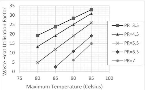
Figure 8 shows the relationship between waste heat utilisation factor and the maximum temperature. The waste heat recovery factor is unaffected by the presence of a recuperator, as the shape of the T-s diagram remains the same, the only thing that changes is the source of the heat for the first part of the heat addition segment. The pinch point analysis for the hot water remains the same.
[image:5.595.305.557.49.206.2]
The data show that the waste heat utilisation factor increases with increasing temperature, but decreases for increasing pressure ratio. There is also an increasing sensitivity to changes in pressure ratio at lower temperatures.
[image:5.595.46.293.303.501.2]Fig. 6: Variation of Second Law Efficiency with Maximum Temperature (with recuperator). PR denotes expander pressure ratio.
Fig. 7: Variation of Second Law Efficiency with Maximum Temperature (without recuperator). PR denotes expander pressure ratio.
Fig. 8: Variation of Waste Heat Utilisation Factor with Maximum Temperature. PR denotes expander pressure ratio.
This can be explained by the fact that the waste heat utilisation factor is tied to the mass flow rate of hot water. The higher the mass flow rate of hot water for a given power output, the lower this factor is.
When there is a large superheat, the slope of the Temperature-Energy plot of the hot water can be relatively large and still maintain the appropriate temperature differential with the working fluid at the evaporator inlet and pinch point. When there is a smaller superheat, a far greater flow rate of hot water is required to ensure that the pinch point temperature difference remains sufficiently large. At very small values of superheat, small changes can cause large differences to the slope, due to being proportionally more significant. This explains why at lower temperatures and higher pressures, the waste heat utilisation factor is lower, and also more sensitive to changes.
V. DISCUSSION AND CONCLUSION
The implications of the results generated by the computer model vary depending on the application for which the ORC system is to be used. The trend of the results is that the amount of superheat at point 3 is determined by both the temperature of the heat source, and the evaporator pressure. Higher values of evaporator pressure and lower values of maximum temperature lower the amount of superheat. In turn, the amount of superheat affects the mass flow rate of hot water required to maintain both appropriate temperature differentials inside the evaporator, and the desired power output, and therefore the waste heat recovery factor of the system. The significance of this fact depends strongly on the application for which the Organic Rankine Cycle is being used.
If, for example, it has been retrofitted to recover energy from a hot process stream, the waste heat utilisation factor is relatively important, as any waste heat not recovered by the Organic Rankine Cycle will be lost, dumped into the environment. In this situation, it is best to sacrifice some of the first and second law efficiency of the Organic Rankine Cycle in order to utilize more of the available heat.
If, on the other hand, the heat source is a solar or geothermal collector, the primary working fluid is generally recirculated instead of being released. This means that any heat not used by the Organic Rankine Cycle will simply result in a higher inlet temperature at the collector, meaning 0
10 20 30 40 50 60 70
75 80 85 90 95 100
Second
Law
Efficiency
Maximum Temperature
PR=3.5
PR=4.5
PR=5.5
PR=6.5
PR=7
0 10 20 30 40 50 60
75 80 85 90 95 100
Second
Law
Efficiency
Maximum Temperature
PR=3.5
PR=4.5
PR=5.5
PR=6.5
PR=7
0 5 10 15 20 25 30 35
75 80 85 90 95 100
Waste
Heat
Utilisation
Factor
Maximum Temperature (Celsius)
[image:5.595.47.293.538.714.2]less energy needs to be transferred, and reducing required heat exchanger areas. In this case, the amount of energy recovered from the hot water is of less concern.
REFERENCES
[1] HUNG, T. C.; SHAI, T. Y.; WANG, S. K. A Review of Organic Rankine Cycles (ORCs) for the Recovery of Low Grade Waste Heat.
Energy, v. 22, n. 7, 1997.
[2] HUNG, T. C. Waste Heat Recovery of Organic Rankine cycle Using Dry Fluids. Energy Conversion and Management, v. 42, n. 5, 2001.
[3] ROY, J. P.; MISHRA, M. K.; MISRA, A. "Parametric optimization and performance analysis of a waste heat recovery system using Organic Rankine Cycle". Energy, v. 35, n. 12, 2010.
[4] WANG, L. D.; ZHAO, L. "Analysis of zeotropic mixtures used in low-temperature solar Rankine cycles for power generation". Solar Energy, v. 83, n. 5, 2009.
[5] MANOLAKOSA, D. et al. Experimental evaluation of an autonomous low-temperature solar Rankine cycle system for reverse osmosis desalination. Desalination, v. 203, n. 1-3, 2006.
[6] HETTIARACHCHIA, H. D. M. et al. Optimum Design Criteria for an Organic Rankine Cycle using Low-Temperature Geothermal Heat Sources. Energy, v. 32, n. 9, 2007.
[7] GAWLIK, K.; HASSANI, V. Advanced Binary Cycles: Optimum Working Fluids. National Renewable Energy Laboratory. [S.l.]. 1998.
[8] DRESCHER, U.; BRÜGGEMANN, D. Fluid selection for the Organic Rankine Cycle (ORC) in biomass power and heat plants.
Applied Thermal Engineering, v. 27, n. 1, 2007.
[9] LIU, H.; SHAO, Y.; LI, J. A biomass-fired micro-scale CHP system with organic Rankine cycle (ORC) – Thermodynamic modelling studies. Biomass and Bioenergy, v. 35, n. 9, 2011.
[10] GUOQUAN QIU, H. L. S. R. Expanders for micro-CHP systems with organic Rankine cycle. Applied Thermal Engineering, v. 31, n. 16, 2011.
[11] QUOILIN, S.; LEMORT, V.; LEBRUN, J. Experimental study and modeling of an Organic Rankine Cycle using scroll expander.
Applied Energy, v. 87, 2010.
[12] BAO, J.; ZHAO, L. A review of working fluid and expander selections for organic Rankine cycle. Renewable and Sustainable Energy Reviews, v. 24, 2013.
[13] QIU, G.; LIU, H.; RIFFAT, S. Expanders for micro-CHP systems with organic Rankine cycle. Applied Thermal Engineering, v. 31, 2011.
[14] DECLAYE, S. et al. Experimental study on an open-drive scroll expander integrated into an ORC (Organic Rankine Cycle) system with R245fa as working fluid. Energy, v. 55, 2013.
[15] WANG, X. D. et al. Performance Evaluation of a Low-Temperature Solar Organic Rankine Cycle System utilising R245fa. Solar Energy, 2009.
[16] GUO, C. et al. Performance analysis of organic Rankine cycle based on location of Pinch Point in Evaporator. Applied Thermal Engineering, v. 62, n. 1, 2014.
[17] LI, Y.-R.; WANG, J.-N.; DU, M.-T. Influence of coupled pinch point temperature difference and evaporation temperature on performance of Organic Rankine Cycle. Energy, v. 42, n. 1, 2012.
[18] WANG, D.; LING, X.; PENG, H. Performance analysis of double organic Rankine cycle for discontinuous low temperature waste heat recovery. Applied Thermal Engineering, v. 48, 2012.
[19] KAUSHIK, O. K.; SINGH, C. S. Energy And Exergy Analysis and Optimisation of Kalina Cycle Coupled with a Coal Fired Steam Power Plant. Applied Thermal Engineering, v. 51, 2013.
[20] KANG, S. H. Design and experimental study of ORC (organic Rankine cycle) and radial turbine using R245fa working fluid.