Data Engineering by the Best
`
1
Convex Data
Fitting Method
S. S. Papakonstantinou and I. C. Demetriou
Abstract—We consider the application of a method that makes the least sum of absolute value change to measured values of a convex function contaminated with random errors to achieve convexity. Thus, we present how to analyze, summarize and interpret these data. The method uses an algorithm of descent direction that employs Karush-Kuhn-Tucker like parameters that are both important to the characterization of the solution and useful for sensitivity analysis. Convexity is expressed in terms of non-negative second divided differences of the smoothed data, which gives a linear programming calculation that is subsequently solved by this algorithm. The data set that is employed for illustration is the time series of the annual Gini coefficients in the U.S.A. from 1947 to 1996. The results are analyzed and the interpretation capability of the method is demonstrated.
Index Terms—convex data fitting, diminishing return, divided difference,`1 approximation, linear programming
I. INTRODUCTION
W
hat hypotheses can be made about the nature of a convex function, which is known only by a set of measured values that have lost convexity due to errors of measurement? The answer to this question has strong ties with many applications of economics, science, engineering and medicine. Applications in economics, for example, arise when assuming diminishing rates of change of certain de-mand and production relations [14]. In medical imaging and robotic vision applications, convex polygonal curves are recovered from measurements of convex sets that include errors by optimizing some measure of performance [11]. Other examples arise from univariate convex data fitting, from decision making [13] and biology [8], for instance. In particular, the method may be used in order to explore possible convex relationships between the variables in mul-tivariate data analysis, thus providing a useful companion to data exploration methodologies.The purpose of this paper is to present how to analyze, summarize and interpret a set of measured values of a convex function f(x) contaminated with random errors by the use of a `1 data approximation method that minimizes the sum
of the moduli of the errors subject to the condition that the second divided differences of the smoothed data are nonnegative. There are many advantages to using `1 data
approximation techniques in practice (see, for example, [15]) and this paper is an aid to application of a specific `1
algorithm for achieving convexity.
The data are the pairs(xi, φi),i= 1,2, . . . , n, where the abscissae xi, i = 1,2, . . . , n satisfy the inequalities x1 <
Manuscript received April 10, 2014.
S. S. Papakonstantinou is with the Department of Economics, University of Athens, 8 Pesmazoglou street, Athens 10559, Greece, e-mail: [email protected]
I. C. Demetriou is with the Department of Economics, Univer-sity of Athens, 8 Pesmazoglou street, Athens 10559, Greece, e-mail: [email protected]
x2<· · ·< xn, andφiis the measurementf(xi). We assume
thatφi=f(xi) +εi, whereεiis a random number. We also assume that there are some gross errors in the data due to blunders.
The authors [17] addressed the problem of calculating numbers yi,i= 1,2, . . . , n from the measurements that are smooth and closer than the measurements to the true function values. They regarded the original data and the smoothed values as vectorsφandy respectively inRn and considered the problem of minimizing the objective function
φ−y1= n X
i=1
|φi−yi|, y∈Rn, (1)
subject to the convexity constraints
y[xi−1, xi, xi+1]≥0, i= 2,3, . . . , n−1, (2)
where
y[xi−1, xi, xi+1] =
yi−1
(xi−1−xi)(xi−1−xi+1)
+
yi
(xi−xi−1)(xi−xi+1)
+ yi+1
(xi+1−xi−1)(xi+1−xi)
(3)
is the ith second divided difference on the components of
y (see [19] for a definition). We call feasible any vector in
Rnthat satisfies the constraints (2). The constraints onyare linear, we denote the constraint normals with respect toyby
aj,j= 2,3, . . . , n−1 and we let
y[xj−1, xj, xj+1] =aTjy, j= 2,3, . . . , n−1. (4)
Also, we let aij be the ith component of aj. Since each divided difference depends on only 3 adjacent components ofy, it immediately follows that the constraints have linearly independent normals.
Since (1) is continuous in y and tends to infinity as
y
1−→ ∞for feasibley and the set of feasible vectors is
closed, a finite solution exists. We call it a best`1convex fit
toφ. Since (1) is not strictly convex, the solution need not be unique.
In view of [12], this problem may also be derived when the data come from processes that show increasing rates of change (cf. convexity), but one does not have sufficient information to set up a parametric form for the underlying function. Thus, by writing theith second divided difference in the form
y[xi−1, xi, xi+1] =
y[xi, xi+1]−y[xi−1, xi] xi+1−xi−1
, (5)
where
y[xi−1, xi] =
yi−yi−1
xi−xi−1
is theith first divided difference, the inequalities on the rates of change of the sequence {yi : i= 1,2, . . . , n}
yi−yi−1
xi−xi−1
≤ yi+1−yi
xi+1−xi
, i= 2,3, . . . , n−1 (7)
imply the inequalities (2). Therefore, an alternative expres-sion of the constraints (2) is that we require increasing rates of change on [x1, xn], a property that is quite common
in describing processes, where a potential shape for the underlying function is that of a convex curve.
The piecewise linear interpolant through the points
(xi, yi), i = 1,2, . . . , n provides some useful geometric description. If all the differences (2) are zero, then the smoothed values lie on a straight line. Otherwise some divided differences are positive, which makes this interpolant be a convex polygonal curve. It is interesting to note that the knots of this polygon are a subset of the abscissae which are not known in advance, but they are calculated automatically from the process. Further, ifn >4and if the data lie on two straight lines in the shape of letter “V” with one of the data at the vertex, then no other convex function can interpolate them [5].
Besides that the shape of convexity is likely to strike immediately a user’s eye when he inspects the data, two properties of this calculation, which provide some advantages over other smoothing techniques [3], are as follows. There is no need to choose a set of approximating functions, because the missing property of convexity is imposed as a smoothing condition, namely inequalities (2), in an optimization calcula-tion that undertakes the process. The approximacalcula-tion process is a projection because, if the data satisfy the convexity constraints, then the data provide the required approximation. Similar problems are studied and characterized by [23], where (1) is replaced by the supremum norm
φ−y
∞= max1≤i≤n|φi−yi| (8)
and by [7], where (1) is replaced by the least squares norm
φ−y2= v u u t
n X
i=1
(φi−yi)2. (9)
Expression (8) is appropriate when the data errors have a uniform distribution, while expression (9) is appropriate when the data errors have a normal distribution. Methods that rely upon (1) are well suited to long tailed error distributions, like Cauchy or Laplace, and have the remarkable property of ignoring some gross errors in the data that makes it “markedly superior among the Lp norms” as [21] states.
For a general reference on `1 approximation from finite
dimensional subspaces see [18].
The paper is organized as follows. In Section II charac-terization conditions are stated, which resemble the Karush-Kuhn-Tucker conditions, that are important both in theory and in developing efficient algorithms. The associated La-grange multipliers as well as some other parameters derived from the optimal fit are highly informative for practical analyses and applications of the problem. In Section III the method is applied to the times series of the Gini coefficients in the U.S.A. for the period 1947-1996. An optimal fit is calculated, the values of the mentioned multipliers and parameters are considered and several features of the data
are revealed. This example is worked out as an illustration of the optimality conditions that a best`1convex fit satisfies.
A similar analysis may well be applied to a variety of situations which may arise in several fields. Finally, some concluding remarks are presented in Section IV. Based on the characterization conditions, the authors have developed an algorithm of descent direction and one of the authors [16] has implemented the method in Matlab. The program consists of about 200 lines including a simple driver, which gives an idea of the size of the required calculation in this environment.
Because sometimes it would be better to employ non-positive instead of nonnegative second divided differences, the method may be applied after a change of sign of the components ofφ, which implies diminishing rates of change (cf. concavity) of the sequence{yi: i= 1,2, . . . , n}, giving
the inequalities
yi−yi−1
xi−xi−1
≥ yi+1−yi
xi+1−xi
, i= 2,3, . . . , n−1. (10)
II. BEST`1DATAFITTING SUBJECT TONONNEGATIVE
SECONDDIVIDEDDIFFERENCES
The general`1 linear approximation problem may be
for-mulated as a primal or a dual linear programming calculation [1], [2]. These formulations allow certain characterization theorems and specific numerical methods [9] for implement-ing the simplex method [6]. Therefore, it is straightforward to minimize the objective function (1) subject to the convexity constraints (2) by using a standard simplex method. However, because several thousand data points may occur in many smoothing calculations, a special technique for this problem has been developed by the authors using search of directions of descent [22] and taking into account the structure of the constraints. This method gains an order of magnitude over the classical simplex approaches, both in storage and in number of operations during the iterations.
LetAbe a nonempty subset of{2,3, . . . , n−1}and let|A| be the number of elements ofA. The problem that minimizes (1) subject to the equality or active constraints
y[xi−1, xi, xi+1] = 0, i∈A, (11)
has particular interest to the inequality constrained problem of Section I. It is a discrete`1approximation problem from
the linear subspace defined by the equations (11) to the finite set of values {φi, i = 1,2, . . . , n}. It always has a
solution, which could be determined by interpolation to some components ofφ, as the following theorem shows.
Theorem 1: There exists a vector y that minimizes (1) subject to the constraints (11) and that has the property
yi=φi, i∈I⊆ {1,2, . . . , n}, (12)
with setI containing at leastn− |A|indices.
Proof: A proof that is based on [20] is provided by [17].
The theorem states that a best`1fity toφsubject to (11)
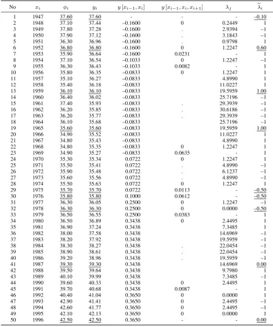
TABLE I
BEST`1CONVEX FIT TO THEGINI COEFFICIENTS FOR THE TIME PERIOD1947-1996,CALCULATED DIFFERENCES AND OPTIMAL PARAMETERS
No xi φi yi y[xi−1, xi] y[xi−1, xi, xi+1] λj eλi
1 1947 37.60 37.60 - - - –0.10
2 1948 37.10 37.44 –0.1600 0 0.2449 1 3 1949 37.80 37.28 –0.1600 . 2.9394 –1 4 1950 37.90 37.12 –0.1600 . 3.1843 –1 5 1951 36.30 36.96 –0.1600 . 0.9798 1 6 1952 36.80 36.80 –0.1600 0 1.2247 0.60 7 1953 35.90 36.64 –0.1600 0.0231 - 1 8 1954 37.10 36.54 –0.1033 0 1.2247 –1 9 1955 36.30 36.43 –0.1033 0.0082 - 1 10 1956 35.80 36.35 –0.0833 0 1.2247 1 11 1957 35.10 36.27 –0.0833 4.8990 1 12 1958 35.40 36.18 –0.0833 11.0227 1 13 1959 36.10 36.10 –0.0833 19.5959 1.00 14 1960 36.40 36.02 –0.0833 25.7196 –1 15 1961 37.40 35.93 –0.0833 . 29.3939 –1 16 1962 36.20 35.85 –0.0833 . 30.6186 –1 17 1963 36.20 35.77 –0.0833 . 29.3939 –1 18 1964 36.10 35.68 –0.0833 25.7196 –1 19 1965 35.60 35.60 –0.0833 19.5959 1.00 20 1966 34.90 35.52 –0.0833 11.0227 1 21 1967 34.80 35.43 –0.0833 4.8990 1 22 1968 34.80 35.35 –0.0833 0 1.2247 1 23 1969 34.90 35.27 –0.0833 0.0635 - 1 24 1970 35.30 35.34 0.0722 0 1.2247 1 25 1971 35.50 35.41 0.0722 . 4.8990 –1 26 1972 35.90 35.48 0.0722 . 6.1237 –1 27 1973 35.60 35.56 0.0722 . 4.8990 –1 28 1974 35.50 35.63 0.0722 0 1.2247 1 29 1975 35.70 35.70 0.0722 0.0113 - –0.50 30 1976 35.80 35.80 0.1000 0.0612 - –0.50 31 1977 36.30 36.05 0.2500 0 1.2247 –1 32 1978 36.30 36.30 0.2500 0 0.0000 –0.50 33 1979 36.50 36.55 0.2500 0.0383 - 1 34 1980 36.50 36.89 0.3438 0 2.4495 1 35 1981 36.90 37.24 0.3438 7.3485 1 36 1982 38.00 37.58 0.3438 14.6969 –1 37 1983 38.20 37.92 0.3438 19.5959 –1 38 1984 38.30 38.27 0.3438 . 22.0454 –1 39 1985 38.90 38.61 0.3438 . 22.0454 –1 40 1986 39.20 38.96 0.3438 . 19.5959 –1 41 1987 39.30 39.30 0.3438 14.6969 0.00 42 1988 39.50 39.64 0.3438 9.7980 1 43 1989 40.10 39.99 0.3438 7.3485 –1 44 1990 39.60 40.33 0.3438 0 2.4495 1 45 1991 39.70 40.68 0.3438 0.0087 - 1 46 1992 40.40 41.04 0.3650 0 0.0000 1 47 1993 42.90 41.41 0.3650 0 2.4495 –1 48 1994 42.60 41.77 0.3650 0 2.4495 –1 49 1995 42.10 42.13 0.3650 0 0.0000 1 50 1996 42.50 42.50 0.3650 - - 0.00
needed that should also test the optimality of a trial set of interpolation points [19]. The following theorem provides optimality conditions for this problem.
Theorem 2: Letsi be the sign of yi−φi,
si=
−1, φi> yi
0, φi=yi i= 1,2, . . . , n
1, φi< yi.
A vector y∈Rn minimizes (1) subject to (11) if and only if there exists a vectorv in
V ={v∈Rn: |v
i| ≤1, i∈I; vi=si, i /∈I} (13)
such that
yTv= 0. (14)
Proof: See Theorem 6.1 of [24].
Therefore in order thaty minimizes (1) subject to (11), it suffices to find a vectorv inV that is orthogonal to y.
Furthermore, in order to minimize (1) subject to (2), Theorem 1 suggests searching for a best `1 fit among
feasible (i.e. convex) vectors that satisfy the interpolation conditions (12). Therefore several applications of Theorem 2 may be needed before a solution is reached. Theorem 3 below provides conditions for testing whether a feasible vector that satisfies the conditions of Theorem 1 is optimal [17]. It is remarkable that although the objective function (1) is non-differentiable, these conditions are given in terms of Karush-Kuhn-Tucker description.
(1) subject to (2), if and only if there exist nonnegative multipliersλj,j∈A, such that
s∗i =X j∈A
λjaij, i /∈I. (15)
Motivated by this theorem we write v as a linear combi-nation of the constraint normals aj,j∈A,
v=X
j∈A
λjaj, (16)
which, in view of (11), satisfies the orthogonality condition (14) and, in view of (15), satisfies the relationsvi=si, i /∈I
that appear in (13). In addition, by invoking the separating hyperplane theorem (see, for example, [25]), it can be proved that a vector y∗ minimizes (1) subject to (11) if and only if
−1≤vi≤1, i∈I. (17)
Hence, the construction of v is complete. Further, for nota-tional purposes, we letλie =vi, for i= 1,2, . . . , n.
The parameters λj andeλi are important to the
develop-ment of an algorithm of descent direction, both for adding and deleting interpolation points, and for deleting from and adding to the active set constraints iteratively until the conditions of Theorem 3 are satisfied.
III. DATA ENGINEERING BY THE BEST`1CONVEX FIT
METHOD
In this section we analyze, summarize and interpret the results obtained by a best `1 convex fit to a particular data
set, which shows a convex pattern. Specifically, the data are the values of the Gini coefficient and its evolution in the U.S.A. for the time period 1947 to 1996. The same data set is used by [10]. The Gini coefficient is commonly used as a measure of inequality of income or wealth [4], where a value of 0 expresses total equality and a value of 100 maximal inequality. Fifty pairs of data were retrieved from the World Income Inequality Database of the U.S. Bureau of Census 1997 and presented in the second (xi) and third (φi) column of Table I. The interest here does not lie on any theoretical assumption of convexity nor on any underlying relation that has to be validated, but on explaining numerically what is happening with the optimality conditions of the calculated best `1 convex fit to the data. Furthermore, we are not
interested in the physical details of the process, but only in what they imply for the convex relationship.
The data were fed to the computer program without any preliminary analysis. The initial components for y were set to the line that interpolates the points (x1, φ1) and
(x50, φ50)and the solution was reached with the set of data
interpolation indicesI={1,6,13,19,29,30,32,41,50}and the set of indices of active constraintsA={2,3, . . . ,49} \ {7,9,23,29,30,33,45}. The components of the calculated best`1 convex fit are presented in the fourth column (yi) of
Table I and displayed in Fig.1. Index 6 ∈ I implies the interpolation condition y6 = φ6 = 36.80. Index 6 ∈ A
implies the active constraint y[x5, x6, x7] = 0. To the
con-trary, since index7∈/A, the 7th constraint is inactive, giving
y[x6, x7, x8] = 0.0231>0. Moreover, the sequences of the
first and the second divided differences of the best convex fit are presented in the fifth and sixth column respectively. They
are useful to the analysis of the results, because they identify and reveal local trends, such as linearities and convexities. The Lagrange multipliers and the components of vector eλ
associated with the best fit are presented in the seventh (λj) and eighth column (eλi) respectively.
1940 1950 1960 1970 1980 1990 2000 34
[image:4.595.299.549.130.328.2]35 36 37 38 39 40 41 42 43
Fig. 1. Best`1 convex fit (o) to the Gini coefficients (+) of Table I for
the years 1947-1996. The piecewise linear interpolant illustrates the fit
Having the setsAandIavailable, the components ofyare defined by interpolation to some components ofφ, in view of (12), and by solving the system of the divided differences that are equal to zero, in view of (11). In case of degeneracy, the inequality|A|+|I|> nmay hold, because setImay contain more thann−|A|elements. Since degeneracy can be avoided in practice, the method arranges the calculation so that|A|+
|I|=n. The solution has given|A|= 41and|I|= 9. Hence the components {yi : i /∈ I} are calculated by solving a
(n− |I|)×(n− |I|)system of equations whose coefficient matrix elements are obtained by deleting a row and column of the n×ncoefficient matrix of the linear equations (11) and (12) for eachi∈ I. This matrix is considered later on when discussing the Lagrange multipliers.
We can immediately notice the non-decreasing property of the sequence of the first divided differences in column 5 as stated by conditions (7). These differences are negative in the interval [1947,1969] and positive subsequently. Therefore, the smoothed Gini coefficients decrease in [1947,1969] down to the value y27 = 35.27 and increase subsequently, with a
rate of change of income inequality that increases gradually from negative to positive values, as it is shown in Table II.
TABLE II
RATES OF CHANGE OFGINI COEFFICIENTS
Period 1st divided differences 1947 - 1953 –0.1600 1953 - 1955 –0.1033 1955 - 1969 –0.0833 1969 - 1975 0.0722 1975 - 1976 0.1000 1976 - 1979 0.2500 1979 - 1991 0.3438 1991 - 1996 0.3650
di-vided differences in column 6 shows the convexity of the piecewise linear interpolant to the smoothed val-ues. Since points with zero second divided differences lie on a straight line and since the positive second di-vided differences are centered at the abscissae with indices {7,9,23,29,30,33,45}, the calculated smoothed values lie on a convex polygonal line that consists of eight consecutive line segments that join the smoothed values at the abscis-sae x1, x7, x9, x23, x29, x30, x33, x45 and x50. The rates of
change shown in Table II are the slopes of the line segments of the piecewise linear interpolant to the smoothed values.
All the Lagrange multipliers in column 7 are nonnegative, according to Theorem 3. We see that whenever λj > 0, then y[xj−1, xj, xj+1] = 0. In words, if the jth Lagrange
multiplier is strictly positive, thejth constraint is by necessity an active constraint at the solution. However, if the jth constraint is strictly positive, then the method ignores the associated jth multiplier. For each vectory=y∗, we obtain the system of equations (15) and we let the corresponding Lagrange multipliers be obtained by solving this system. In words, the columns of the (n− |I|) ×(n − |I|) matrix of system (15) are the normals of the active constraints after deleting the rows for i ∈ I. It is remarkable that the matrix that occurs in the definition of λis the transpose of the matrix that is used to define y. In Fig. 2 we see the coefficient matrix of (15), emphasizing its sparsity. The first row of numbers displays the indices of the active constraints, namelyA. The first column of numbers displays the data in-dices after excluding the interpolation point inin-dices, namely {1,2, . . . ,50} \I. Because the abscissae are equally spaced and because multiplication of this matrix by a constant does not change the problem, the matrix elements in Fig. 2 come from the coefficients of the second difference giving a quint diagonal band and similarly if the abscissae are not equally spaced. The higher the value of a Lagrange multiplier, the stronger the linear tendency of the corresponding constraint is. The symmetric values of the Lagrange multipliers ob-served in the intervals[1956,1968]and[1980,1990]are due to the local symmetries of the coefficient matrix of system (15) and the distribution of the±1signs at the constant side of this system.
In view of the zero Lagrange multipliers λ32 = λ46
= λ49 = 0 and the corresponding zero differences
y[x31, x32, x33] = y[x45, x46, x47] = y[x48, x49, x50] = 0,
we deduce that the obtained best`1convex fit is degenerate.
Hence, the minimization of the objective function (1) subject to the active constraints that are indexed in setAleads to the same best fit, whether any of the constraints with index32,
46or49is present or not. For example, whether we impose the constraint y[x31, x32, x33] ≥0 or not and then proceed
to minimize (1) subject to the remaining constraints indexed in setA, we obtain a solution which happens to satisfy the equation y[x31, x32, x33] = 0. Similarly, whether we impose
y[x45, x46, x47]≥0 or not, the result is the same.
The best fit interpolates the points (xi, yi), for i ∈
{1,6,13,19,29,30,32,41,50}. The associated parameters
e
λi in column 8 of Table I have the values λe1 = −0.10,
e
λ6 = 0.60, eλ13 = 1.00, λe19 = 1.00, eλ29 = −0.50,
e
λ30 =−0.50, λe32 = −0.50, eλ41 = 0.00 andλe50 = 0.00,
which are all in the interval [−1,1] as it follows from the optimality conditions (17). The underlined components ofφ,
y andeλin Table I indicate the interpolation point positions
and the correspondingλie. The components{eλi: i /∈I}have
the values of the signs of the residuals yi−φi, according to the equations contained in (13), and the components {λie :i∈I} are obtained from formula (16) for i∈I. The
corresponding 9×41 coefficient matrix in (16) for i ∈ I, say it is ΣT, is presented below in transposed form. The first row of numbers displays the indices in set I and the first column of numbers displays the indices in set A. In words,ΣT consists of the rows excluded from the formation
of the matrix in Fig. 2. Further, the underlined components of eλi, i ∈ I in column 8 of Table I, in view of (16) for i∈I, are obtained by multiplyingΣT with the vector whose
components are the active constraint multipliers λj, j ∈A
(see column 7 of Table I).
Σ =
1 6 13 19 29 30 32 41 50
2 1 0 0 0 0 0 0 0 0
3 0 0 0 0 0 0 0 0 0
4 0 0 0 0 0 0 0 0 0
5 0 1 0 0 0 0 0 0 0
6 0 −2 0 0 0 0 0 0 0
8 0 0 0 0 0 0 0 0 0
10 0 0 0 0 0 0 0 0 0
11 0 0 0 0 0 0 0 0 0
12 0 0 1 0 0 0 0 0 0
13 0 0 −2 0 0 0 0 0 0
14 0 0 1 0 0 0 0 0 0
15 0 0 0 0 0 0 0 0 0
16 0 0 0 0 0 0 0 0 0
17 0 0 0 0 0 0 0 0 0
18 0 0 0 1 0 0 0 0 0
19 0 0 0 −2 0 0 0 0 0
20 0 0 0 1 0 0 0 0 0
21 0 0 0 0 0 0 0 0 0
22 0 0 0 0 0 0 0 0 0
24 0 0 0 0 0 0 0 0 0
25 0 0 0 0 0 0 0 0 0
26 0 0 0 0 0 0 0 0 0
27 0 0 0 0 0 0 0 0 0
28 0 0 0 0 1 0 0 0 0
31 0 0 0 0 0 1 1 0 0
32 0 0 0 0 0 0 −2 0 0
34 0 0 0 0 0 0 0 0 0
35 0 0 0 0 0 0 0 0 0
36 0 0 0 0 0 0 0 0 0
37 0 0 0 0 0 0 0 0 0
38 0 0 0 0 0 0 0 0 0
39 0 0 0 0 0 0 0 0 0
40 0 0 0 0 0 0 0 1 0
41 0 0 0 0 0 0 0 −2 0
42 0 0 0 0 0 0 0 1 0
43 0 0 0 0 0 0 0 0 0
44 0 0 0 0 0 0 0 0 0
46 0 0 0 0 0 0 0 0 0
47 0 0 0 0 0 0 0 0 0
48 0 0 0 0 0 0 0 0 0
49 0 0 0 0 0 0 0 0 1
IV. CONCLUDINGREMARKS
If measurements of function values show some gross errors and away from them the function seems to be convex, then the least sum of absolute change to the data that provides nonnegative second divided differences may be required. This problem is a highly structured constrained`1
2 3 4 5 6 8 10 11 12 13 14 15 16 17 18 19 20 21 22 24 25 26 27 28 31 32 34 35 36 37 38 39 40 41 42 43 44 46 47 48 49
2 –2 1 0 0 0 0 0 0 0 0 0 0 0 0 0 0 0 0 0 0 0 0 0 0 0 0 0 0 0 0 0 0 0 0 0 0 0 0 0 0 0 3 1 –2 1 0 0 0 0 0 0 0 0 0 0 0 0 0 0 0 0 0 0 0 0 0 0 0 0 0 0 0 0 0 0 0 0 0 0 0 0 0 0 4 0 1 –2 1 0 0 0 0 0 0 0 0 0 0 0 0 0 0 0 0 0 0 0 0 0 0 0 0 0 0 0 0 0 0 0 0 0 0 0 0 0 5 0 0 1 –2 1 0 0 0 0 0 0 0 0 0 0 0 0 0 0 0 0 0 0 0 0 0 0 0 0 0 0 0 0 0 0 0 0 0 0 0 0 7 0 0 0 0 1 1 0 0 0 0 0 0 0 0 0 0 0 0 0 0 0 0 0 0 0 0 0 0 0 0 0 0 0 0 0 0 0 0 0 0 0 8 0 0 0 0 0 –2 0 0 0 0 0 0 0 0 0 0 0 0 0 0 0 0 0 0 0 0 0 0 0 0 0 0 0 0 0 0 0 0 0 0 0 9 0 0 0 0 0 1 1 0 0 0 0 0 0 0 0 0 0 0 0 0 0 0 0 0 0 0 0 0 0 0 0 0 0 0 0 0 0 0 0 0 0 10 0 0 0 0 0 0 –2 1 0 0 0 0 0 0 0 0 0 0 0 0 0 0 0 0 0 0 0 0 0 0 0 0 0 0 0 0 0 0 0 0 0 11 0 0 0 0 0 0 1 –2 1 0 0 0 0 0 0 0 0 0 0 0 0 0 0 0 0 0 0 0 0 0 0 0 0 0 0 0 0 0 0 0 0 12 0 0 0 0 0 0 0 1 –2 1 0 0 0 0 0 0 0 0 0 0 0 0 0 0 0 0 0 0 0 0 0 0 0 0 0 0 0 0 0 0 0 14 0 0 0 0 0 0 0 0 0 1 –2 1 0 0 0 0 0 0 0 0 0 0 0 0 0 0 0 0 0 0 0 0 0 0 0 0 0 0 0 0 0 15 0 0 0 0 0 0 0 0 0 0 1 –2 1 0 0 0 0 0 0 0 0 0 0 0 0 0 0 0 0 0 0 0 0 0 0 0 0 0 0 0 0 16 0 0 0 0 0 0 0 0 0 0 0 1 –2 1 0 0 0 0 0 0 0 0 0 0 0 0 0 0 0 0 0 0 0 0 0 0 0 0 0 0 0 17 0 0 0 0 0 0 0 0 0 0 0 0 1 –2 1 0 0 0 0 0 0 0 0 0 0 0 0 0 0 0 0 0 0 0 0 0 0 0 0 0 0 18 0 0 0 0 0 0 0 0 0 0 0 0 0 1 –2 1 0 0 0 0 0 0 0 0 0 0 0 0 0 0 0 0 0 0 0 0 0 0 0 0 0 20 0 0 0 0 0 0 0 0 0 0 0 0 0 0 0 1 –2 1 0 0 0 0 0 0 0 0 0 0 0 0 0 0 0 0 0 0 0 0 0 0 0 21 0 0 0 0 0 0 0 0 0 0 0 0 0 0 0 0 1 –2 1 0 0 0 0 0 0 0 0 0 0 0 0 0 0 0 0 0 0 0 0 0 0 22 0 0 0 0 0 0 0 0 0 0 0 0 0 0 0 0 0 1 –2 0 0 0 0 0 0 0 0 0 0 0 0 0 0 0 0 0 0 0 0 0 0 23 0 0 0 0 0 0 0 0 0 0 0 0 0 0 0 0 0 0 1 1 0 0 0 0 0 0 0 0 0 0 0 0 0 0 0 0 0 0 0 0 0 24 0 0 0 0 0 0 0 0 0 0 0 0 0 0 0 0 0 0 0 –2 1 0 0 0 0 0 0 0 0 0 0 0 0 0 0 0 0 0 0 0 0 25 0 0 0 0 0 0 0 0 0 0 0 0 0 0 0 0 0 0 0 1 –2 1 0 0 0 0 0 0 0 0 0 0 0 0 0 0 0 0 0 0 0 26 0 0 0 0 0 0 0 0 0 0 0 0 0 0 0 0 0 0 0 0 1 –2 1 0 0 0 0 0 0 0 0 0 0 0 0 0 0 0 0 0 0 27 0 0 0 0 0 0 0 0 0 0 0 0 0 0 0 0 0 0 0 0 0 1 –2 1 0 0 0 0 0 0 0 0 0 0 0 0 0 0 0 0 0 28 0 0 0 0 0 0 0 0 0 0 0 0 0 0 0 0 0 0 0 0 0 0 1 –2 0 0 0 0 0 0 0 0 0 0 0 0 0 0 0 0 0 31 0 0 0 0 0 0 0 0 0 0 0 0 0 0 0 0 0 0 0 0 0 0 0 0 –2 1 0 0 0 0 0 0 0 0 0 0 0 0 0 0 0 33 0 0 0 0 0 0 0 0 0 0 0 0 0 0 0 0 0 0 0 0 0 0 0 0 0 1 1 0 0 0 0 0 0 0 0 0 0 0 0 0 0 34 0 0 0 0 0 0 0 0 0 0 0 0 0 0 0 0 0 0 0 0 0 0 0 0 0 0 –2 1 0 0 0 0 0 0 0 0 0 0 0 0 0 35 0 0 0 0 0 0 0 0 0 0 0 0 0 0 0 0 0 0 0 0 0 0 0 0 0 0 1 –2 1 0 0 0 0 0 0 0 0 0 0 0 0 36 0 0 0 0 0 0 0 0 0 0 0 0 0 0 0 0 0 0 0 0 0 0 0 0 0 0 0 1 –2 1 0 0 0 0 0 0 0 0 0 0 0 37 0 0 0 0 0 0 0 0 0 0 0 0 0 0 0 0 0 0 0 0 0 0 0 0 0 0 0 0 1 –2 1 0 0 0 0 0 0 0 0 0 0 38 0 0 0 0 0 0 0 0 0 0 0 0 0 0 0 0 0 0 0 0 0 0 0 0 0 0 0 0 0 1 –2 1 0 0 0 0 0 0 0 0 0 39 0 0 0 0 0 0 0 0 0 0 0 0 0 0 0 0 0 0 0 0 0 0 0 0 0 0 0 0 0 0 1 –2 1 0 0 0 0 0 0 0 0 40 0 0 0 0 0 0 0 0 0 0 0 0 0 0 0 0 0 0 0 0 0 0 0 0 0 0 0 0 0 0 0 1 –2 1 0 0 0 0 0 0 0 42 0 0 0 0 0 0 0 0 0 0 0 0 0 0 0 0 0 0 0 0 0 0 0 0 0 0 0 0 0 0 0 0 0 1 –2 1 0 0 0 0 0 43 0 0 0 0 0 0 0 0 0 0 0 0 0 0 0 0 0 0 0 0 0 0 0 0 0 0 0 0 0 0 0 0 0 0 1 –2 1 0 0 0 0 44 0 0 0 0 0 0 0 0 0 0 0 0 0 0 0 0 0 0 0 0 0 0 0 0 0 0 0 0 0 0 0 0 0 0 0 1 –2 0 0 0 0 45 0 0 0 0 0 0 0 0 0 0 0 0 0 0 0 0 0 0 0 0 0 0 0 0 0 0 0 0 0 0 0 0 0 0 0 0 1 1 0 0 0 46 0 0 0 0 0 0 0 0 0 0 0 0 0 0 0 0 0 0 0 0 0 0 0 0 0 0 0 0 0 0 0 0 0 0 0 0 0 –2 1 0 0 47 0 0 0 0 0 0 0 0 0 0 0 0 0 0 0 0 0 0 0 0 0 0 0 0 0 0 0 0 0 0 0 0 0 0 0 0 0 1 –2 1 0 48 0 0 0 0 0 0 0 0 0 0 0 0 0 0 0 0 0 0 0 0 0 0 0 0 0 0 0 0 0 0 0 0 0 0 0 0 0 0 1 –2 1 49 0 0 0 0 0 0 0 0 0 0 0 0 0 0 0 0 0 0 0 0 0 0 0 0 0 0 0 0 0 0 0 0 0 0 0 0 0 0 0 1 –2
Fig. 2. The coefficient matrix of system (15)
the general approach may arise in several fields. Moreover, the subject deserves study in the area of inferential statistics in order to bring about further possibilities for applications.
ACKNOWLEDGMENT
This work was supported in part by the University of Athens under Research Grant 11105.
REFERENCES
[1] I. Barrodale and F. D. K. Roberts, “An improved algorithm for discrete `1linear approximation”,SIAM J. Numer. Anal., vol. 10, pp. 839-848,
1973.
[2] I. Barrodale and F. D. K. Roberts, “An efficient algorithm for discrete `1linear approximation with linear constraints”,SIAM J. Numer. Anal.,
vol. 15, pp. 603-611, 1978.
[3] C. de Boor,A Practical Guide to Splines. Revised Edition, NY: Springer-Verlag, Applied Mathematical Sciences, vol. 27, 2001.
[4] S. R. Chakravarty,Ethical Social Index Numbers, NY: Springer-Verlag, 1990.
[5] M. P. Cullinan, “Data smoothing using non-negative divided differences and `2 approximation”,IMA J. Numer. Anal., vol. 10, pp. 583-608,
1990.
[6] G. B. Dantzig,Linear Programming and Extensions, Princeton, New Jersey: Princeton University Press, 1968.
[7] I. C. Demetriou and M. J. D. Powell, “The minimum sum of squares change to univariate data that gives convexity”,IMA J. Numer. Anal., vol. 11, pp. 433-448, 1991.
[8] K. R. Foster, “Diminishing returns in social evolution: the not-so-tragic commons”,J. Evol. Biol., vol. 17, pp. 1058-1072, 2004.
[9] R. Fletcher,Practical Methods of Optimization, Chichester, England: J. Wiley & Sons, 2003.
[10] S. A. Georgiadou and I. C. Demetriou, “The Karush-Kuhn-Tucker test of convexity of univariate observations and certain economic applications”,IAENG Int. J. Appl. Math., vol. 38, 1, pp. 44-53, 2008.
[11] N. I. Fisher, P. Hall, B. A. Turlach and G. S. Watson, “On the estimation of a convex set from noisy data on its support function”, J. of Amer. Stat. Assoc., vol. 92, 43, pp. 84-91, 1997.
[12] C. Hildreth, “Point estimates of ordinates of concave functions”,J. of Amer. Stat. Assoc., vol. 49, pp. 598-619, 1954.
[13] D. V. Lindley,Making Decisions, 2nd Edition, London, England: J. Wiley & Sons, 1985.
[14] C. J. McKenna and R. Rees,Economics: A Mathematical Introduction, Oxford, England: Oxford University Press, 1996.
[15] M. R. Osborne,Finite Algorithms in Optimization and Data Analysis, Chichester, England: J. Wiley & Sons, 1985.
[16] S. S. Papakonstantinou,Discrete`1Approximation subject to
Increas-ing Returns and Applications to Economic Data, Ph.D. Dissertation, Division of Mathematics and Informatics, Department of Economics, University of Athens, Athens, Greece, 2012.
[17] S. S. Papakonstantinou and I. C. Demetriou, “Necessary and sufficient conditions for best L1 estimates of ordinates of convex functions”,
IAENG Int. J. Appl. Math., vol. 38, 1, pp. 30-33, 2008.
[18] A. M. Pinkus,OnL1-approximation, Cambridge, England: Cambridge University Press, 1989.
[19] M. J. D. Powell, Approximation Theory and Methods, Cambridge, England: Cambridge University Press, 1981.
[20] J. R. Rice,The Approximation of Functions. Vol. 1, Reading, Mass.: Addison-Wesley, 1964.
[21] J. R. Rice and J. S. White, “Norms for smoothing and estimation”, SIAM Review, vol. 6, 3, pp. 243-256, 1964.
[22] M. Shi and M. A. Lukas, “AnL1estimation algorithm with degeneracy
and linear constraints”,Comp. Stat. & Data Anal., vol. 39, pp. 35-55, 2002.
[23] V. A. Ubhaya, “An O(n) algorithm for discrete n-point convex approximation with applications to continuous case”,J. of Math. and Appl. Anal., vol. 72, pp. 338-354, 1979.
[24] G. A. Watson,Approximation Theory and Numerical Methods, Chich-ester, England: J. Wiley & Sons, 1980.