Homogenization of an Optimal Control Problem in
Fixed Domains
Jake Avila, Bituin Cabarrubias
Abstract—This work deals with the asymptotic behavior of an optimal control problem based on an elliptic boundary value problem with a linear Robin boundary condition posed in a fixed domain. We consider an L2-cost functional and use the Periodic Unfolding Method to homogenize the problem. We also show that under this method, the energy corresponding to this cost functional converges. Moreover, we obtain estimates satisfied by the state and control variables.
Index Terms—elliptic problem, homogenization, Robin con-dition, optimal control, unfolding method.
I. INTRODUCTION
I
N this paper, we study the homogenization of an optimal control problem based on a linear elliptic boundary value problem with highly oscillating coefficients posed in a fixed domain. The boundary is assumed to be Lipschitz contin-uous with a prescribed linear Robin condition. An L2-cost functional is considered in this work.Optimal controls and homogenization both have a lot of applications in many different fields such as aerospace, process control, robotics, bioengineering, economics, fi-nance, management science, filtration, geomechanics and soil mechanics, petroleum and construction engineering, geo-sciences, biomedicine and biophysics, among others. The goal of this paper is to yield a new model that can be used in describing some physical phenomenon or in producing a new material for advanced technologies. As far as the authors know, this study is the first in this area.
To study the asymptotic behavior of the problem, we use the Periodic Unfolding Method (PUM), a recently designed technique of homogenization that was first introduced in [6] (see [7] for the detailed proofs and to [14] for an elementary approach) for fixed domains. This technique was extended to perforated domains in [9] (see also [10] for the proofs and [11] for additional applications). One can also check [12] when one wants to consider more general situations and comprehensive presentation and [17] for time-dependent functions. This method was also further stretched to domains with small holes in [13] (see also [27]) and to domain with small holes for time-dependent functions in [5].
As for the homogenization of optimal control problems governed by a linear elliptic equation with linear Robin boundary condition on perforated domains via PUM by considering two types of cost functionals, the reader is referred to [4]. For the asymptotic behavior of the optimal controls based on the wave equation with homogeneous
Manuscript received April 13, 2017; revised April 21, 2017.
J. Avila is an undergraduate student of the Institute of Mathematics, University of the Philippines Diliman, 1101 Diliman, Quezon City, PHILIP-PINES e-mail: [email protected].
B. Cabarrubias is an assistant professor in the Institute of Mathematics, University of the Philippines Diliman, 1101 Diliman, Quezon City, PHILIP-PINES e-mail: [email protected].
Neumann boundary condition in domains with oscillating boundary and via some compactness properties and evolution triples, see [15]. In [16], the asymptotic behavior of a quasilinear optimal control problem with thick multilevel junction was considered by passing to the limit in the adjoint problem and by using the Γ−convergence (see [2] and [3] for this technique). The reader is also referred to [18] for the homogenization of an optimal control problem posed in perforated and nonperforated domains via this convergence. As for the multi-scale convergence andH−convergence (see [1] for this method) one can check [19] and [20] and [22], respectively. For additional works and applications in this area, the reader is referred to [24], [25], [26], [28] and [30]. This paper is organized as follows: Section II is devoted to the short discussion on PUM for fixed domains, Section III presents the problem, the optimal control results and estimates while Section IV contains the convergence results.
II. PERIODICUNFOLDINGMETHOD FORFIXED DOMAINS
Let us recall here some notations, definition of the unfold-ing operator and some of its properties as given in [7].
LetΩbe an open set andb= (b1, b2, . . . , bN)be a basis of RN. Let Y be a reference cell or a set possessing the
paving property with respect tob. For z ∈ RN, we denote by [z]Y =
N X
j=1
kjbj the unique
integer combination of periods with the property thatz−[z]Y belongs toY, and by{z}Y the difference
{z}Y =z−[z]Y.
This means,
[image:1.595.301.497.542.767.2]z={z}Y + [z]Y, z∈RN.
Fig. 1. {z}Y and[z]Y . Thus, we can write
x=εnx ε o
Y
+hx
ε i
Y
,
We also use the notations
Ξε=ξ∈ZN, ε(ξ+Y)⊂Ω ,
b
Ωε=interior
[
ξ∈ZN
ε(ξ+Y)
,
Λε= Ω\Ωbε.
[image:2.595.53.286.544.755.2]Here, one hasΩbεthe interior of the largest union of the cells ε(ξ+Y)such thatε(ξ+Y)is fully contained inΩandΛε represents the parts from the cells ε(ξ+Y) that intersects the boundary∂Ω(see the figure below).
Fig. 2. Ωbε (brown) andΛε (light green)
We have the following definition of the unfolding operator.
DEFINITION 1. Let ϕ be aLebesgue-measurable function onΩ. Define the unfolding operatorTε as
Tε(ϕ)(x, y) =ϕ
εhx ε i
Y
+εy,
a.e. for (x, y)∈Ωbε×Y and
Tε(ϕ)(x, y) = 0,
a.e. for (x, y)∈Λε×Y.
REMARK 2. From this definition, it follows that Tε(v w)(x, y) =Tε(v)(x, y)Tε(w)(x, y),
for v andwLebesgue-measurable functions.
Some properties of the unfolding operator needed in this work are given in the following theorem.
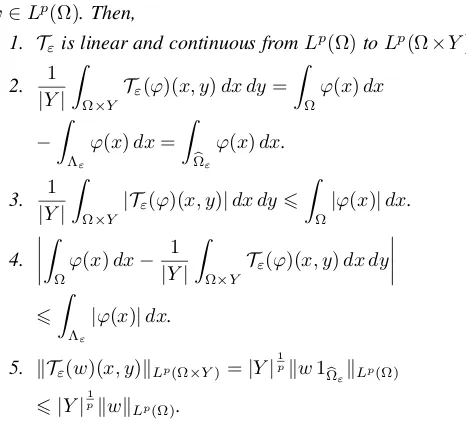
THEOREM 3. Let p > 1 and is finite, ϕ ∈ L1(Ω), and w∈Lp(Ω). Then,
1. Tεis linear and continuous fromLp(Ω)toLp(Ω×Y).
2. 1 |Y|
Z
Ω×Y
Tε(ϕ)(x, y)dx dy= Z
Ω
ϕ(x)dx
− Z
Λε
ϕ(x)dx=
Z
b Ωε
ϕ(x)dx.
3. 1 |Y|
Z
Ω×Y
|Tε(ϕ)(x, y)|dx dy6 Z
Ω
|ϕ(x)|dx.
4.
Z
Ω
ϕ(x)dx− 1 |Y|
Z
Ω×Y
Tε(ϕ)(x, y)dx dy
6 Z
Λε
|ϕ(x)|dx.
5. kTε(w)(x, y)kLp(Ω×Y)=|Y|
1
pkw1 b ΩεkLp(Ω)
6|Y|p1kwk Lp(Ω).
One has the following criterion called the unfolding crite-rion for integrals.
THEOREM 4. If the sequence{ϕε}inL1(Ω) satisfies Z
Λε
|ϕε(x)|dx→0,
then
Z
Ω
ϕε(x)dx− 1 |Y|
Z
Ω×Y
Tε(ϕε)(x, y)dx dy→0.
Moreover, we write
Z
Ω
ϕε(x)dxT'ε 1 |Y|
Z
Ω×Y
Tε(ϕε)(x, y)dx dy.
The following convergence properties of the unfolding operator are very essential in the homogenization of the problem.
THEOREM 5. Let 1≤p <∞. 1. Forw∈Lp(Ω),
Tε(w)→w inLp(Ω×Y).
2. Let{wε} be a sequence inLp(Ω)such that
wε→w inLp(Ω).
Then,
Tε(w)→w inLp(Ω×Y).
COROLLARY 6. Let 1< p <∞, and{wε} be a sequence converging weakly inW1,p(Ω) tow. Then
Tε(wε)* w w-Lp(Ω;W1,p(Y)).
THEOREM 7. Let p >1 and is finite. If wε * w weakly in W1,p(Ω), then there exists
b
w ∈ Lp(Ω;W1,p
per(Y)) with
MY(wb) = 0such that up to a subsequence,
Tε(∇wε)*∇w+∇ywbw-L
p(Ω×Y).
III. STATEMENT OF THEPROBLEM ANDOPTIMAL CONTROLRESULTS
LetM(α, β,Ω)denote the set ofN×N matrix fields
A= (aij)1≤i,j≤N ∈(L∞(Ω))N×N,
satisfying
(A(y)λ, λ)≥α|λ|2
and |A(y)λ| ≤β|λ|,
for all λ ∈ RN and a.e. in Ω with 0 < α < β for real
numbersαandβ.
Consider the spaceH1(Ω) equipped with the norm
kvkH1(Ω)=
kvk2L2(Ω)+k∇vk
2 L2(Ω)
12
. (1)
Letε >0. We want to study the asymptotic behaviour of the optimal control governed by the linear elliptic problem with linear Robin boundary condition given by,
(
−div(Aε∇u
ε) =f+θ inΩ,
Aε∇u
ε·~n+hεuε=g on ∂Ω,
(2)
situated in the fixed domainΩ where~n is the exterior unit normal vector to Ω. We suppose that the boundary ∂Ω is Lipschitz continuous and the data satisfy:
A1. f andθ are functions inL2(Ω). A2. g is a function inL2(∂Ω).
A4. Aε(x) =A x ε
such that A∈ M(α, β,Ω). The variational formulation of (2) is given by
For everyε >0, find uε∈H1(Ω) such that Z
Ω
Aε∇uε∇v dx+
Z
∂Ω
hεuεv ds=
Z
Ω f v dx
+
Z
Ω
θv dx+
Z
∂Ω
gv ds, ∀v∈H1(Ω).
(3)
We have the following property due to Lax-Milgram Theorem.
THEOREM8. The variational problem (3) admits a unique solution.
Let us now consider the L2-cost functional given by
Jε(uε, θ) =
1 2
Z
Ω
(uε−ud) 2
dx+ν 2
Z
Ω θ2dx,
where ud ∈ L2(Ω) is the desired state independent of ε, and ν >0 is the functional’s regularization parameter. The optimal control problem forJε(uε, θ)is given by
Fε:inf
Jε(uε, θ)|θ∈L2(Ω),(uε, θ)satisfies (3) .
This problem is standard and we have:
PROPOSITION 9. For each ε > 0, problem Fε admits a unique solution.
We also have the following property which characterizes the optimal control.
PROPOSITION10. Let(¯uε,θ¯)be the optimal solution ofFε
and let the adjoint state pε¯ satisfy the problem
(
−div(tAε∇p¯
ε) = ¯uε−ud in Ω,
tAε∇pε¯ ·~n+hεpε.¯ = 0 on∂Ω.
Then the optimal controlθ¯ε is given byθ¯ε=−1νp¯ε.
Conversely, if the pair(uε,b −1
νpεb)∈H
1(Ω)×H1(Ω)solves
the optimality system
−div(Aε∇ b
uε) =f−1νpbε in Ω, Aε∇
b
uε·~n+hεuεb =g on∂Ω,
−div(tAε∇ b
pε) =buε−ud in Ω,
tAε∇ b
pε·~n+hεpεb = 0 on∂Ω,
then the pair (buε,−1
νbpε) is the optimal solution ofFε.
For the proofs of Proposition 9 and Proposition 10, one can follow the arguments for e.g., in [21] and [29].
PROPOSITION 11. Let (¯uε,θε¯) be the optimal solution of
Fε, andpε¯ be the adjoint state. Then we have the estimates,
kpε¯ kH1(Ω)6C,
kθ¯εkL2(Ω)6C,
and
k¯uεkH1(Ω)6C,
whereC is a generic positive constant independent of ε.
IV. HOMOGENIZATIONRESULTS
In this section, we present the homogenization results we obtained via periodic unfolding method. We start with the limit problem corresponding to problem (2).
Consider the spaceH1
0(Ω)together with the norm defined in (1) and the problem
(
−div(A0∇u) =f+θ inΩ,
u= 0 on∂Ω. (4)
with the following assumptions: H1. f andθ are functions inL2(Ω). H2. A0∈ M(α0, β0,Ω), where α0, β0∈
Rwith
0< α0< β0.
An immediate consequence of the Lax-Milgram Theorem is the following proposition.
PROPOSITION12. Problem (4) admits a unique solution u
inH1
0(Ω) that satisfies the a priori estimate
kukH1
0(Ω)6C, for some positive constantC.
Now, let us have theL2-cost functional given by
J(u, θ) = 1 2
Z
Ω
(u−ud)2 dx+ν 2
Z
Ω θ2dx,
where ud ∈ L2(Ω) is the desired state, and ν > 0 is the functional’s regularization parameter. The optimal control problem forJ(u, θ)is
F :inf
J(u, θ)|θ∈L2(Ω),(u, θ)satisfies(4) .
PROPOSITION 13. Problem F admits a unique optimal solution (¯u,θ¯), where u¯ is the optimal state andθ¯is the optimal control.
To characterize the optimal control, we have:
PROPOSITION 14. Let (¯u,θ¯)be the optimal solution of F
and let the adjoint statep¯satisfy the problem
(
−div(tA0∇p¯) = ¯u−ud inΩ,
¯
p= 0 on∂Ω, (5)
then the optimal control is given byθ¯=−1 νp¯.
Conversely, if the pair(bu,−1 νpb)∈H
1
0(Ω)×H01(Ω) solves
the optimality system
−div(A0∇ b
u) =f−1
νpb inΩ,
b
u= 0 on∂Ω,
−div(tA0∇ b
p) =bu−ud inΩ,
b
p= 0 on∂Ω,
(6)
then the pair(u,b −1
νpb)is the optimal solution ofF.
One can prove Proposition 13 and Proposition 14, again, by following the steps done in in [21] and [29].
We now have the following convergence results obtained via PUM.
THEOREM 15. Let (¯uε,θε¯ )be the optimal solution ofFε
with the adjoint statepε¯ . If there exists a matrix field A in M(α, β,Ω×Y)such that
then there exist u, p∈H1
0(Ω) and θ∈L2(Ω) such that up
to subsequences, f¯
uε * u w-H1(Ω),
fpε¯ * p w-H 1(Ω),
fθ¯ε * θ w-L2(Ω),
(8)
and (u, p, θ) ∈ H1
0(Ω) ×H01(Ω)×L2(Ω) is the unique
solution to the optimality system
−div(A0∇u) =f+θ inΩ,
u= 0 on∂Ω
−div(tA0∇p) =u−u
d inΩ, p= 0 on∂Ω.
(9)
The homogenized matrix fieldsA0and tA0are constant and
elliptic, and are given by
A0=M
Y(aij)− MY n X
k=1 aik
∂χcj(y) ∂yk
!
tA0=M
Y(aij)− MY n X
k=1
akj∂χi(y) ∂yk
! ,
(10)
for almost every y ∈ Y, and for all λ ∈ RN, χjb is the
solution to
−div(A∇χλb ) =−div(Aλ) in Y A∇(χbλ−λ·y)·n= 0 on ∂Ω
b
χλ beY-periodic MY(χbλ) = 0,
(11)
and χi is the solution to
−div(tA∇χλ) =−div(tAλ) in Y tA∇(χ
λ−λ·y)·n= 0 on∂Ω χλ be Y-periodic
MY(χλ) = 0.
(12)
Moreover, there existbu,pb∈L2(Ω;H1
per(Y))withMY(bu) =
0 and MY(pb) = 0, such that up to subsequences,
Tε(¯uε)* u w-L2(Ω;H1(Y))
Tε(∇u¯ε)*∇xu+∇yub w-L
2(Ω×Y)
Tε(¯pε)* p w-L2(Ω;H1(Y))
Tε(∇p¯ε)*∇xp+∇ypb w-L
2(Ω×Y)
Tε(¯θε)* θ w-L2(Ω;H1(Y)), (13)
where(u, p,u,b bp, θ)is the unique solution to the limit equa-tion
∀ϕ∈H1(Ω), ψ∈L2(Ω;Hper1 (Y)),
1 |Y|
Z
Ω×Y
A(∇xu+∇yub)(∇xϕ+∇yψ(x, y))dx dy
=
Z
Ω
(f+θ)ϕ dx
1 |Y|
Z
Ω×Y tA(∇
xp+∇ybp)(∇xϕ+∇yψ(x, y))dx dy
=
Z
Ω
(u−ud)ϕ dx.
(14)
Outline of the Proof: The convergences in (8) follow from the estimates given in Proposition 10. Those in (13) are due to Proposition 11, Corollary 6 and Theorem 7. The limit equation in (14) can be derived by considering two types of test functions in the variational problem and applying the unfolding operator together with its properties given in Section II.
Finally, we have the following convergence of the energy corresponding to theL2-cost functionalJ
ε(uε, θ).
THEOREM 16. Let (¯uε,θ¯ε) and p¯ε, and (¯u,θ¯) and p¯
be the optimal solutions and adjoint states of Fε and F,
respectively. Then,
(i) fuε¯ *u¯ w-H 1(Ω),
(ii) fpε¯ *p¯ w-H 1(Ω),
(iii) fθ¯ε *θ¯ w-L2(Ω).
(15)
Moreover,
lim
ε→0Jε(¯uε,
¯
θε) =J(¯u,θ¯). (16)
REFERENCES
[1] M. Briane, A. Damlamian and P. Donato, “H-convergence in perforated domains” in Non-linear partial Differential Equations and Their Appli-cations, Coll´ege de France seminar vol. XIII, D. Cioranescu and J. L. Lions eds., Pitman Research Notes in Mathematics Series, Longman, New York, (391) (1998), 62-100.
[2] G. Buttazzo and G. Dal Maso, “Γ-convergence and optimal control problems”, Journal of Optimization Theory and Applications, Vol 38, No. 3, (1982), 385-407.
[3] G. Buttazzo, “Γ-convergence and its applications to some problem in the calculus of variations”, in School on Homogenization, ICTP, Trieste, 1993 (1994) 3861.
[4] B. Cabarrubias, “Homogenization of optimal control problems in per-forated domains via periodic unfolding method”, Applicable Analysis, 95:11, (2016) 2517-2534, DOI:10.1080/00036811.2015.1094799. [5] B. Cabarrubias and P. Donato, “Homogenization of some evolution
problems in domains with small holes”, Electronic Journal of Differen-tial Equations, Vol. 2016, No. 169 (2016), 1-26.
[6] D. Cioranescu, A. Damlamian and G. Griso, “Periodic unfolding and homogenization”,C.R. Acad. Sci. Paris, Ser. I 335, pp. 99-104, 2002. [7] D. Cioranescu, A. Damlamian and G. Griso, “The periodic unfolding
and homogenization”,SIAM J. Math. Anal., Vol. 40, No. 4, pp. 1585-1620, 2008.
[8] D. Cioranescu and P. Donato, “Homog´en´esation du probl`eme de Neu-mann non homog`ene dans des ouverts perfor´es”,Asymptotic Anal.Vol. 1, pp. 115-138, 1988.
[9] D. Cioranescu, P. Donato and R. Zaki, “The Periodic Unfolding and Robin problems in perforated domains”,C.R.A.S. Paris, S´erie 1, 342, pp. 467-474, 2006.
[10] D. Cioranescu, P. Donato and R. Zaki, “The Periodic Unfolding Method in Perforated Domains”,Portugal Math 63(4), pp. 476-496, 2006.
[11] D. Cioranescu, P. Donato and R. Zaki, “Asymptotic behavior of elliptic problems in perforated domains with nonlinear boundary conditions”,
Asymptotic Analysis53, pp. 209-235, 2007.
[12] D. Cioranescu, A. Damlamian, P. Donato, G. Griso and R. Zaki, “The Periodic Unfolding Method in Domains With Holes”,SIAM J. Math. Anal., Vol. 44, No. 2, pp. 718-760, 2012.
[13] D. Cioranescu, A. Damlamian, G. Griso and D. Onofrei, The periodic unfolding method for perforated domains and Neumann sieve models, J. Math. Pures Appl. 89 (2008), 248-277.
[14] A. Damalamian, “An elementary introduction to periodic unfolding”,
Gakuto International Series, Math.Sci. Appl.Vol. 24, pp. 119-136, 2005. [15] T. Durante, L. Faella and C. Perugia, “Homogenization and behavior of optimal controls for the wave equation in domains with oscillating boundary”, Nonlinear Differ. Equ. Appl. 14 (2007), 455489. [16] T. Durante and T.A. Melnyk, “Homogenization of quasilinear optimal
control problem involving a thick multilevel junction of type 3:2:1”, ESAIM Control Optim. Calc. Var. 18(2) (2012), 583610.
[18] S. Kesavan and T. Muthukumar, “Homogenization of an optimal con-trol problem with state constraints”, Differ. Equ. Dyn. Syst. 19(4)(2011), 361-374.
[19] S. Kesavan and M. Rajesh, “Homogenization of periodic optimal control problems via multi-scale convergence”, Proc. Indian Acad. Sci. (Math. Sci.), VOl. 108, No.2, (1998) 189-207.
[20] ] S. Kesavan and J. Saint Jean Paulin, “Optimal control on perforated domains”, J. Math. Anal. Appl. 229, (1999), 563-586.
[21] J.-L.Lions,Optimal control of systems governed by partial differential equations,Springer-Verlag, Berlin 1971.
[22] T. Muthukumar and A.K. Nandakumaran, “Homogenization of low-cost control problems on perforated domains”, J. Math. Anal. Appl. 351 (2009), 29-42.
[23] A.K. Nandakumaran, R. Prakash and B.C. Sardar, “Homogenization of an optimal control problem in a domain with highly oscillating boundary using periodic unfolding method”, MESA, Vol.4, No.3, (2013) 281-303.
[24] A.K. Nandakumaran and R. Prakash, “Homogenization of Bound-ary Optimal Control Problems with Oscillating BoundBound-ary”, Nonlinear Studies-The International Journal, Vol. 20, No. 3, pp. 1-25, 2013. [25] A.K. Nandakumaran, R. Prakash and J.P. Raymond, “Asymptotic
analysis and error estimates for an optimal control problem with oscillating boundaries”, Ann. Univ. Ferrara, 58 (2012), 143-166. [26] A.K. Nandakumaran, R. Prakash and J-P Raymond, “Stokes System in
a Domain with Oscillating Boundary: Homogenization and Error Anal-ysis of an Interior Optimal Control Problem”, Numerical Functional Analysis and Optimization, 20l3.
[27] D. Onofrei, “The unfolding operator near a hyperplane and its appli-cation to the Neumann Sieve model”, AMSA, 16 (2006), 239-258. [28] R. Prakash, “Optimal Control Problem for the Time-Dependent
Kirchhoff-Love Plate in a Domain with Rough Boundary”, Asymptotic Analysis 81 (2013) 337-355.
[29] J.P. Raymond,Optimal control of partial differential equations, Univer-sit`e Paul Sabatier, www.math.univ-toulouse.fr.
![Fig. 1. {z}Y and [z]Y .Thus, we can write](https://thumb-us.123doks.com/thumbv2/123dok_us/415266.539081/1.595.301.497.542.767/fig-y-and-y-thus-we-can-write.webp)