Abstract—In these days, the online monitoring information which includes usage history, system conditions, and environmental conditions is reported. On statistical modeling, these variables from the online monitoring are primary candidates for covariates which affect the failure mechanism. There is some literature on modeling by the cumulative exposure model for a products lifetime distribution with covariate effects. Some existing literatures require an already known parametric baseline distribution of the cumulative exposure. However such knowledge may be difficult to acquire in advance in some cases. When an incorrect baseline distribution is assumed, it is called misspecification. A previous study proposed the strategy which use a likelihood function under a log-normal distribution to estimate parameters which represent covariate effects when the truly underlying baseline distribution is either a Weibull distribution or a log-normal distribution. In this time, my paper widens the range of application of the strategy using the likelihood function under a log-normal distribution to estimate parameters of covariate effects. On that account, the simulation study and the discussion for the bias of estimation are shown.
Index Terms—Log-normal distribution, Gamma distribution, Birnbaum-Saunders distribution, Cumulative exposure, Misspecification
I. INTRODUCTION
NLINE monitoring using the Internet has become a common tool for keeping products reliably. This information includes usage history and environmental conditions. In the statistical modeling of failure mechanisms, the variables contained in this information are primary candidates for covariates that affect a failure mechanism. Information on covariates can be used to improve a reliability analysis. For example, in the analysis of the lifetime distribution of a truck engine, the lifetime is usually estimated on the basis of the distance traveled (mileage) before catastrophic failure. However, other variables observed by each truck, such as an average slope of the routes traveled and an average weight of the loads carried, affect the load on the engine. Thus, the load on the engine can differ even though the mileage is the same. Therefore, the mileage is not always sufficient information for optimizing inspection and maintenance times.
Manuscript received July 10, 2015; revised July 29, 2015. This work was supported by a Grant-in-Aid for Young Scientists (B) (No. 15K16301) from the Japan Society for the Promotion of Science.
Masahiro Yokoyama is an assistant professor at the Department of Industrial and Systems Engineering at Chuo University, Japan e-mail: ([email protected]).
II. PREVIOUS STUDIES AND MY PROPOSAL A. Previous Studies
In [1] and [2], the utilization of dynamic covariate to predict field-failure is presented. They used the cumulative exposure (CE) model to describe an effect of a dynamic covariate on the failure-time distribution. Reference [3] and [4] described the CE model in the context of life tests to incorporate time-varying covariates into failure-time models. The CE model is also known as the cumulative damage (CD) model, in [5]. Besides, reference [6] called the CE model a “proportional quantities (PQ) model” or a “scale accelerated failure-time (SAFT) model.” Furthermore, it is remarked that the CE model can be considered as a limit of the step-stress model when the length of each step interval goes to zero, in [4].
Given the entire covariate history, the cumulative exposure u by time t defined as
t s ds
t t u
0
tr ( )] .
exp[ )]
( , ;
[ βz β z (1)
Here, β is a vector of covariate parameters (acceleration coefficients) and z(t) is a covariate vector acquired at continuous time point t, and tr represents transposed. The value of the covariates are either discrete or continuous. Equation (1) represents a nonlinear transformation of t to quantity u, which incorporates dynamic covariate information of individual user’s products with the conventional lifetime analysis.
Let T be the failure time of the unit and β*be the true value
of β. The unit fails at time T when the amount of cumulative exposure reaches a random threshold U(β*). Thus, the
relationship between the cumulative exposure U(β*) and the
failure time T is
T
ds s U
0 tr *
*) exp[ ( )] .
(β β z (2)
The cumulative exposure threshold U(β*) has the baseline
cumulative distribution function (cdf) F0(U) with distribution
parameter θ0. Equation (2) represents an accumulation of
damage. Thus, in this model, if the product is heavily used or used in a harsh environment, the product fails sooner.
For this approach based on the CE model, the baseline distribution F0(U) is needed to identify in advance. In [1], a
Weibull distribution is used for the CE of actual products and it is said that engineering knowledge based on laboratory tests, previous experience with similar failure modes, or knowledge
A Study on Estimation of Lifetime Distribution
with Covariates Under Misspecification
Masahiro Yokoyama, Member, IAENG
of the physics of failure can also provide useful information to identify the baseline distribution. As a special case, the baseline distribution is the same as the distribution of the product failure time T, when it is used under a constant covariates. However consumer products are used under various environment and the CE value U(β*) cannot be
observed. There is a research about a statistical test to identify the baseline distribution in the context of accelerated failure time models, in [7]. On the other hand, some study focus on the estimation bias of β under misspecification for the baseline distribution F0(U). [8] proposed a strategy and its
validity to use a likelihood function under a log-normal distribution to estimate the covariate effects parameter β when the underlying distribution for F0(U) is assumed a
Weibull distribution or a log-normal distribution. With this approach, a model can be built that incorporates covariates even if a Weibull baseline distribution is misspecified as a log-normal one.
B. My Proposal
For the estimation of β under misspecification, this research widen the scope of the type of distribution from [8]. In this research, two-parameter gamma distribution and Birnbaum-Saunders (Fatigue Life) distribution are considered. This paper proposes a strategy and its validity to use a likelihood function under a log-normal distribution to estimate the covariate effects parameter β when the underlying distribution for F0(U) which is assumed a gamma
distribution and a Birnbaum-Saunders (Fatigue Life) distribution. With this approach, a model can be built that incorporates covariates even if a gamma and Birnbaum-Saunders baseline distribution is misspecified as a log-normal one. This study makes the lifetime prediction for individual user’s products using the observed covariates easy to use.
The gamma distribution is commonly used in reliability analysis for cases where partial failures can exist, i.e., when a given number of partial failures must occur before an item fails (e.g., redundant systems). For example, the gamma distribution can describe the time for an electrical component to fail. The general formula for the probability density function of the gamma distribution without reference to the location parameter is
, 0 , , ) (
) exp( ) ( ) (
1
m m
x f
x m x
G
where m is the shape parameter, η is the scale parameter, and Γ is the gamma function.
The Birnbaum-Saunders distribution is also commonly known as the fatigue life distribution. The assumption of the Birnbaum-Saunders distribution is consistent with a deterministic model from materials physics known as Miner's rule. Miner’s rule is one of the most widely used cumulative damage models for failures caused by fatigue. When the physics of failure suggests Miner's rule applies, the Birnbaum-Saunders model is a reasonable choice for a lifetime distribution model. The formula for the probability density function and cumulative distribution function of the Birnbaum-Saunders distribution without reference to the location parameter are
, 0 , , 2
)
(
m m
mx x
f x
x x x BS
and ( ) , , 0,
m m
x
F x
x BS
where m is the shape parameter, η is the scale parameter, φis the probability density function of the standard normal distribution, and Φ is the cumulative distribution function of the standard normal distribution.
III. ANALYTICAL STUDY USING LIKELIHOOD FUNCTION A. Covariate
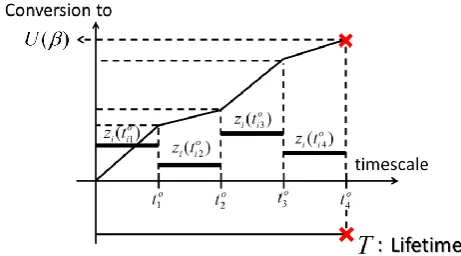
Here we deal with the case in which a target covariate is observed at time tjo (j=1,…,J) for a discrete interval (Fig. 1).
[image:2.595.326.528.297.383.2]The covariate value is assumed to be constant between each pair of tjo.
Fig. 1. Covariate observed at discrete intervals (J=4)
The symbols here used are defined as follows. T Lifetime
tjo Covariate acquisition points ( j=1,…,J )
J Number of covariate acquisition points up to failure
q Covariate type ( q= 1,…,Q,
Q: total number of covariates) zq(tjo) Value of covariate acquired at tjo
[image:2.595.311.542.571.699.2]The nonlinear transformation of lifetime T to quantity U(β) is illustrated in Fig. 2.
Fig. 2. Transformation to U(β)
Let i (i=1,…,n) be the product number of each user, Ti be
the lifetime of each product, z(tijo) be the value of the
observed covariate at tijo for each product, and Ui (β*) be the
B. Likelihood Function
Let μ be the mean and σ be the standard deviation of the log-transformed log-normal distribution. The likelihood function for a log-normal distribution is given by
n i n i o B i LN t i L1 1
,
tr ( ) log( 2 )
) , , (
log β β z
. 2 ) )) ( (log( )) ( log( 1 2 2 1
n i i n i i U U β βThe log-likelihood function for a gamma distribution is given by ) , , (
logLG β m
n i i n i o B
i m U
t i 1 1 , tr )) ( log( ) 1 ( ) ( β z β
( ) log( ) log( ( )).
1 m m U n i
i
β
The log-likelihood function for a Birnbaum-Saunders distribution is given by
) , , (
logLBS βm
n i U U n i o B i i i i t 1 ) ( ) ( 1 , tr log )
( β β
z
β
n i n i i mU 1 1 ) 2 log( )) ( 2log( β
. 2 1 1 2 ) ( ) ( 2
n i U U i i m β β IV. SIMULATION STUDY AND RESULTS A. Simulation Setting
In this simulation study, β was estimated from covariate
z(tijo) and lifetime Tiusing MLE under assuming U(β*) as a
log-normal distribution. These data were generated as explained below.
(1). Ui (β*)
The values of Ui (β*) were generated in accordance with a
log-normal distribution, a gamma distribution or a Birnbaum-Saunders distribution. In section Ⅳ-B, the results of estimation under no misspecification is shown. On the other hand, in section Ⅳ-C, the results of estimation under misspecification for a gamma distribution is shown. Furthermore, in section Ⅳ-D, the results of estimation under misspecification for a Birnbaum-Saunders distribution is shown.
(2). z(tijo)
As was explained above for Fig. 1, the values of z(tijo) was
generated as constant during each observation. We assumed two kinds of covariate; covariates z1(tijo) and z2(tijo) were
independently generated for each product for each observed time point as following a normal distribution N(1.0,0.1), that is taking positive values. Thus, in our simulation, it is assumed that each product is used under a normal condition that time-varying covariates have no trend for time. Here, true values of parameter vector β*=(β
1*, β2*)were set as 1.00 for
both.
(3). Ti
The values of Ti were determined from the Ui (β*) and z(tijo)
generated as described above. The interval between each pair of covariate observations was determined as follows.
1 ) ( , , 2 ) ( ,
1 2 1 , 1 , 2
1 i
o J i o J i o i o i o
i t t t t J
t
i i
(: Interval is increasing by 1.)
i o J i o J
i t J
t
i
i )
( , , 1
(: Interval is less than Ji only for last observation.)
Here,
1 1 2 * 2 1 * 1 * ) ( ) ( exp ) ( i J j o ij o iji z t z t
U β
( ) ( )
( )exp * 2 , , , 1
2 , 1 * 1 o J i o J i o J i o J
i i z t i t i t i
t
z
.
Therefore, lifetime Tifor each product was obtained from the
summation of o J i i
t, .
B. Simulation Results (Log-normal Distribution)
First we show that U(β*) can be correctly estimated using
MLE assuming a log-normal distribution for U(β*) generated
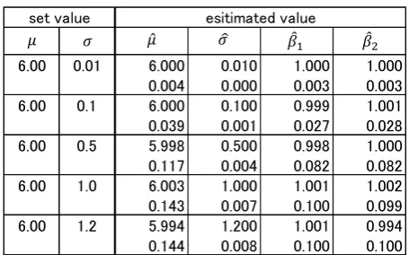
[image:3.595.310.538.484.626.2]in accordance with a log-normal distribution. Table I shows the estimation result of β. The μ and σ represent the set value of the mean value and the standard deviation value of the log-transformed log-normal distribution, respectively. The estimation from simulation data was repeated 2000 times. The results shown in the upper rows are the average estimated values, and those shown in the lower rows are the standard deviations. These results show that the value of β was correctly estimated by MLE.
TABLE I
Estimations obtained for Ui(β*) when Ui(β*) was generated
using a log-normal distribution
(β1*=β2* =1.00, n=10000, no. of repetitions=2000)
6.00 0.01 6.000 0.010 1.000 1.000
0.004 0.000 0.003 0.003
6.00 0.1 6.000 0.100 0.999 1.001
0.039 0.001 0.027 0.028
6.00 0.5 5.998 0.500 0.998 1.000
0.117 0.004 0.082 0.082
6.00 1.0 6.003 1.000 1.001 1.002
0.143 0.007 0.100 0.099
6.00 1.2 5.994 1.200 1.001 0.994
0.144 0.008 0.100 0.100
set value esitimated value
C. Simulation Results (Gamma Distribution)
Here we show that β can be approximately estimated using MLE assuming a log-normal distribution for Ui(β*) generated
in accordance with a gamma distribution. That is, in this simulation study, β is estimated when a gamma distribution is misspecified as a log-normal distribution.
The true value of β was set to 1.00, i.e., β1*=β2* =1.00. The
number of samples n was set as 10000, the shape parameter m was set as 0.8, 1.0, 2.0, 4.0, 6.0 and the location parameter η was set as 200, 400. The estimation of β was repeated 2000 times. Table II and Table III show the mean value and the standard deviations of estimated values.
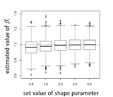
[image:4.595.311.546.52.253.2]The results on Table II and Table III for different distribution assumptions show that parameter β can be approximately obtained. Next, it is investigated that the variation in the estimated results in each value of shape parameter m. Fig. 3 shows a box plot (for η=400, n=10000) of estimation result β1 in Table III.
Fig. 3. Box plot ofestimation result β1 for the case of Table II
(η=100, β1*=β2* =1.00, n=10000, no. of repetitions=2000)
These result shows that when the value of the shape parameter m of the gamma distribution was large, the bias of the resulting estimates of β was small.
D. Simulation Results (Birnbaum-Saunders Distribution)
Here we show that β can be approximately estimated using MLE assuming a log-normal distribution for Ui(β*) generated
in accordance with a Birnbaum-Saunders distribution. That is, in this simulation study, β is estimated when a Birnbaum-Saunders distribution is misspecified as a log-normal distribution.
The true value of β was set to 1.00, i.e., β1*=β2* =1.00. The
number of samples n was set as 10000, the shape parameter m was set as 0.5, 0.8, 1.0, 2.0, 4.0, 6.0 and the location parameter η was set as 200, 400. The estimation of β was repeated 2000 times. Table IV and Table V show the mean value and the standard deviations of estimated values. TABLE II
Estimations obtained for Ui(β*) when Ui(β*) was generated
using a gamma distribution
(β1*=β2* =1.00, n=10000, no. of repetitions=2000)
0.8 200 4.275 1.516 0.969 0.973
0.146 0.017 0.104 0.106
1.0 200 4.667 1.282 0.974 0.973
0.146 0.013 0.099 0.103
2.0 200 5.703 0.803 0.991 0.991
0.140 0.007 0.097 0.099
4.0 200 6.552 0.533 0.996 1.001
0.127 0.004 0.089 0.088
6.0 200 7.003 0.426 1.001 0.998
0.123 0.003 0.087 0.086
set value esitimated value
(The upper column represents mean value of each estimation; the lower column represents standard deviation of each estimation)
TABLE III
Estimations obtained for Ui(β*) when Ui(β*) was generated
using a gamma distribution
(β1*=β2* =1.00, n=10000, no. of repetitions=2000)
0.8 400 4.958 1.516 0.964 0.967
0.146 0.017 0.103 0.100
1.0 400 5.366 1.282 0.979 0.973
0.144 0.013 0.101 0.102
2.0 400 6.398 0.803 0.992 0.992
0.137 0.007 0.098 0.095
4.0 400 7.244 0.533 0.998 0.998
0.128 0.004 0.090 0.093
6.0 400 7.696 0.426 0.998 1.000
0.127 0.003 0.089 0.090
set value esitimated value
(The upper column represents mean value of each estimation; the lower column represents standard deviation of each estimation)
TABLE IV
Estimations obtained for Ui(β*) when Ui(β*) was generated
using a Birnbaum-Saunders distribution (β1*=β2* =1.00, n=10000, no. of repetitions=2000)
0.5 200 5.298 0.486 0.998 1.002
0.110 0.003 0.076 0.078
0.8 200 5.297 0.751 0.997 1.002
0.128 0.005 0.092 0.091
1.0 200 5.297 0.914 0.995 1.003
0.135 0.006 0.093 0.095
2.0 200 5.305 1.591 1.004 1.003
0.146 0.008 0.103 0.099
4.0 200 5.349 2.507 1.022 1.029
0.157 0.011 0.109 0.109
6.0 200 5.322 3.130 1.012 1.012
0.163 0.013 0.111 0.113
set value esitimated value
[image:4.595.308.540.572.738.2]
The results in Table IV and Table V show that parameter β
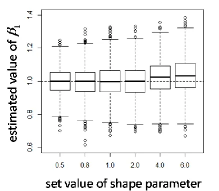
[image:5.595.316.542.58.232.2]can be approximately obtained in the case of misspecification for the Birnbaum-Saunders distribution. Next, it is investigated that the variation in the estimated results in each value of shape parameter m. Fig. 4 shows a box plot (for η=400, n=10000) of estimation result β1 in Table V.
Fig. 4. Box plot ofestimation result β1 for the case of Table V
(η=100, β1*=β2* =1.00, n=10000, no. of repetitions=2000)
These result shows that when the value of the shape parameter m of the Birnbaum-Saunders distribution was small, the bias of the resulting estimates of β was small.
[image:5.595.55.285.107.271.2]However, there is a strange value observed for the mean value of estimation of β in the case of (m=6, η=200) at the Table IV. The cause is that there is many samples that the value of the covariate has not changed even once before failure point in this case, as Fig. 5. Thereby, bias has appeared on the estimation result in this case. Under the normal condition, the covariates are assumed to have changing in time. The validation for the influence due to the observed covariates which has not changed even once before failure point to estimation bias will be with future challenges.
Fig. 5. Number of acquisition points of covariate information up to failure in the case of a certain one estimation under a Birnbaum-Saunders distribution (m=6, η=200, n=10000). In this simulation study, the covariate value is assumed to be constant between each acquisition point.
V. CONCLUSION AND FUTURE WORK
In this section, the strategy under misspecification for a baseline distribution is proposed. This paper investigates the asymptotic bias of the maximum likelihood estimator for a covariate parameter β under misspecification. The results in [9] and [10] also discussed the asymptotic bias and the asymptotic distribution of the MLE when the assumed model is incorrect. Besides, they called this incorrect MLE quasi-MLE (QMLE). From [9], it is shown that a bias between MLE and QMLE is independent for a sample size n. In the case of misspecification that the true model is a gamma distribution or a Birnbaum-Saunders distribution and the incorrect model is a log-normal distribution, the results of numerical simulation show thatcovariate parameter β can be approximately estimated by maximum likelihood estimation assuming a log-normal distribution for the baseline distribution of cumulative exposure.
From the results of numerical simulation for a gamma distribution, it is shown that the value of a location parameter η has no influence for the estimation bias. On the other hand, it is shown that a scale parameter m affects the bias of estimation of covariate parameters β under misspecification. From Table II and Table III, when a shape parameter takes m ≥ 4, it is confirmed that the rate of the bias for the true value (=1.00) is fall under 0.5% in the case of n=10000.
Furthermore, from the results of numerical simulation for a Birnbaum-Saunders distribution, it is shown that the value of a location parameter η has no influence for the estimation bias. On the other hand, it is shown that a scale parameter m affect the bias of estimation of covariate parameters β under misspecification. From the result on Table IV and Table V, when a shape parameter takes m ≤ 2, it is confirmed that the rate of the bias for the true value (=1.00) is fall under 0.5% in the case of n=10000.
Thereby, when the truly underlying baseline distribution is either a gamma distribution or a Birnbaum-Saunders distribution, these results provide a strategy to use a likelihood function under a log-normal distribution to estimate covariate effect parameters β. From the results of numerical simulation, it seems that, if the value of the estimated σ is small, the bias of β is small.
TABLE V
Estimations obtained for Ui(β*) when Ui(β*) was generated
using a Birnbaum-Saunders distribution (β1*=β2* =1.00, n=10000, no. of repetitions=2000)
0.5 400 5.990 0.486 0.999 0.999
0.116 0.003 0.081 0.082
0.8 400 5.987 0.751 0.997 0.998
0.130 0.005 0.092 0.093
1.0 400 5.994 0.914 1.000 1.002
0.137 0.006 0.096 0.097
2.0 400 5.996 1.591 0.999 1.006
0.145 0.008 0.100 0.098
4.0 400 6.035 2.507 1.022 1.021
0.151 0.011 0.105 0.104
6.0 400 6.052 3.130 1.033 1.028
0.160 0.013 0.111 0.111
set value esitimated value
(The upper column represents mean value of each estimation; the lower column represents standard deviation of each estimation)
[image:5.595.55.275.395.586.2]Future work includes finding ways to improve reliability by using online condition monitoring. It will be extended this study to the case of time-varying covariates having trend for time.
REFERENCES
[1] Y. Hong and W. Q. Meeker, “Field-failure predictions based on failure-time data with dynamic covariate information,” Technometrics, vol. 55, no. 2, 2013, pp. 135–149.
[2] W. Q. Meeker and Y. Hong, “Reliability meets big data: Opportunities and challenges,” Quality Engineering, vol. 26, no. 1, 2014, pp. 102-116.
[3] W. Nelson, Accelerated Testing: Statistical Model, Test Plans, and Data Analyzes, New York: John Wiley, 1990.
[4] W. Nelson, “Prediction of field reliability of units, each under differing dynamic stresses, from accelerated test data,” Handbook of Statistics, vol. 20, 2001, pp. 611-621.
[5] V. Bagdonavicius and M. Nikulin, Accelerated Life Models: Modeling and Statistical Analysis. Boca Raton, FL: Chapman & Hall/CRC, 2001.
[6] W. Q. Meeker and L. A. Escobar, Statistical Methods for Reliability Data, New York: John Wiley, 1998.
[7] V. Bagdonavicius, R. Levuliene and M. Nikulin, "Chi-squared goodness-of-fit tests for parametric accelerated failure time models," Communications in Statistics-Theory and Methods, vol. 42, no. 15, 2013, pp. 2768-2785.
[8] M. Yokoyama, W. Yamamoto and K. Suzuki, "A Study on Estimation of Lifetime Distribution with Covariates Using Online Monitoring," Total Quality Science, vol. 1, no. 2, 2015, pp. 89-101.
[9] H. White, "Maximum likelihood estimation of misspecified models," Econometrica, vol. 50, 1982, pp. 1-25.