Exploring the limits of the self consistent Born approximation for inelastic electronic transport

arXiv:0804.3389v1 [cond-mat.other] 21 Apr 2008

transport

William Lee and Stefano Sanvito∗

School of Physics and CRANN, Trinity College, Dublin 2, Ireland

(Dated: February 18, 2013)

The non equilibrium Green function formalism is today the standard computational method for describing elastic transport in molecular devices. This can be extended to include inelastic scattering by the so called self-consistent Born approximation (SCBA), where the interaction of the electrons with the vibrations of the molecule is assumed to be weak and it is treated perturbatively. The validity of such an assumption and therefore of the SCBA is difficult to establish with certainty. In this work we explore the limitations of the SCBA by using a simple tight-binding model with the electron-phonon coupling strengthαchosen as a free parameter. As model devices we consider Au mono-atomic chains and a H2 molecule sandwiched between Pt electrodes. In both cases our

self-consistent calculations demonstrate a breakdown of the SCBA for large αand we identify a weak and strong coupling regime. For weak coupling our SCBA results compare closely with those obtained with exact scattering theory. However in the strong coupling regime large deviations are found. In particular we demonstrate that there is a critical coupling strength, characteristic of the materials system, beyond which multiple self-consistent solutions can be found depending on the initial conditions in the simulation. We attribute these features to the breakdown of the perturbative expansion leading to the SCBA.

I. INTRODUCTION

Central to the field of molecular electronics are phe-nomena involving the interaction between the electron current and the internal degrees of freedom of the molecule investigated. In scanning tunnel microscopy (STM)1,2,3 _{the molecular vibrational modes (phonons)}

have been exploited to desorb or to move a molecule on a surface, paving the way for phonon assisted surface chemistry. At the same time, STM inelastic tunnelling spectroscopy uses the fingerprints of vibrations in the I-V curve to probe the orientation and/or to identity molecules on surfaces4,5,6,7_{. Switching devices exploiting}

phonons have also been reported8_.

Broadly speaking, in molecular devices phonons are important for two reasons. Firstly, they play a role in transport9,10 _{by opening new conductance channels}

through which the itinerant electrons can propagate, and by suppressing the transmission of purely elastic channels11_{. More dramatically, for large electron-phonon}

coupling the charge carriers become quasi-particles con-sisting of coupled electrons and phonons12_{. Secondly,}

from a technological point of view, phonons limit the effi-ciency of molecular devices because of energy dissipation. This causes heating, power loss and instability.

Transport experiments at the nano-scale are difficult to interpret since the atomically precise device geometry is rarely known. Therefore one usually relies on atom-istic simulation techniques in order to understand the results. For elastic transport, when electron-phonon teraction is not considered and the electron-electron in-teraction is treated at the mean field level, methods of note for predicting the current flowing through devices include the non-equilibrium Green function formalism (NEGF)13,14,15,16,17_{and scattering theory (ST)}12,18,19,20_.

Some of these methods have been adapted to include

electron-phonon interaction, notably an extension of scattering theory (EST)11,21,22,23 _{and the self consistent}

Born approximation (SCBA)24,25 _{within the NEGF}

for-malism. In addition time-dependent methods for describ-ing correlated electron-ion dynamics have been recently proposed26_.

The focus of this paper is the SCBA. This is attractive from a practical point of view since it has moderate com-putational requirements and it has been used extensively for calculating transport properties of a number of differ-ent material systems24,25_{. However, it is a perturbative}

approach appropriate only for weak electron-phonon (e-p) coupling. As the e-p coupling strength increases the SCBA will eventually breakdown, however it is unclear whether such breakdown is either sharp or smooth with the e-p coupling strength. Our work explores this ques-tion in detail.

The paper is organized as follows. We begin by pre-senting the NEGF formalism for a two probe device27,28_,

and by recalling the foundations of the SCBA. We then consider a 1D tight-binding model where the e-p inter-action in the scattering region is described by the Su-Schrieffer-Heeger (SSH)29,30 _{Hamiltonian. The}

parame-ters for the model Hamiltonian are chosen for mimicking two systems which have been studied experimentally: H2

molcules sandwiched between Pt electrodes (H2-Pt)9,31

and Au monatomic chains10_{comprising R atoms (RC’s).}

The parameters for H2-Pt are the same as those used

by Jean and Sanvito11_{, who previously employed exact}

II. METHODOLOGY

A. Non Equilibrium Green Function Formalism

A two probe device consists of two crystalline elec-trodes attached on either side of a scattering region, which is in general a collection of atoms breaking the elec-trodes translational symmetry. The leads are also charge reservoirs, so that the device may be viewed as two charge reservoirs bridged by the central region. Thermodynam-ically we characterise the left-hand side (L) and right-hand side (R) lead by defining their chemical potentials µLandµR. IfµL=µR, equilibrium is established and no

current flows. When µL6=µRthe system is dragged out

of equilibrium, and net charge will move from the reser-voir with the higher chemical potential across the central region to the reservoir of lower chemical potential in an attempt to re-establish equilibrium. If a battery is at-tached to the two reservoirs keeping µL−µR = eV (V

is the bias andethe electron charge) the system cannot return to equilibrium and will eventually reach a steady state with a constant current flow.

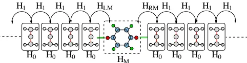
At the Hamiltonian level the problem can be formu-lated by using a basis set comprising a linear combination of atomic orbitals (LCAO). It is convenient to write the Hamiltonian of the semi-infinite periodic leads in term of principal layers (PLs)27,32_{. These are cells that repeat}

periodically and constructed in such a way that the in-teraction between PLs extend only to nearest neighbours (see figure 1). Thus the N ×N matrices H1 and H0

000

111

000

1110110011000110011 001111110000 00 00 11 11 000 000 111 111 00 00 11 11 000 000 111 111 000 000 111 111

H0 H0 H0 H0

00 00 11 11 0 0 1 1 00 11 00 11 0 0 0 1 1 1 00 00 11 11 0 0 1 1 00 00 11 11 00 00 11 11 0 0 1 1 0 0 1 1 0 0 1 1 00 11 00 11 0 0 0 1 1 1 00 00 11 11 00 00 11 11 00 00 11 11 00 00 11 11 0 0 1 1 0 0 1 1 0 0 1 1 00 11 00 11 0 0 0 1 1 1 0 0 1 1 0 0 1 1 00 00 11 11 00 00 11 11 0 0 1 1 00 00 11 11 0 0 1 1 00 11 00 11 0 0 0 1 1 1 0 0 1 1 00 00 11 11 00 00 11 11 00 00 11 11 0 0 1 1

H1 H1 H1 H1 HLM

H0 H0 H0 H0

0 0 1 1 0 0 1 1 00 11 00 11 0 0 0 1 1 1 00 00 11 11 0 0 1 1 00 00 11 11 00 00 11 11 0 0 1 1 0 0 1 1 0 0 1 1 00 11 00 11 0 0 0 1 1 1 00 00 11 11 00 00 11 11 00 00 11 11 00 00 11 11 0 0 1 1 00 00 11 11 0 0 1 1 00 11 00 11 0 0 0 1 1 1 0 0 1 1 0 0 1 1 00 00 11 11 00 00 11 11 0 0 1 1 0 0 1 1 0 0 1 1 00 11 00 11 0 0 0 1 1 1 0 0 1 1 00 00 11 11 00 00 11 11 00 00 11 11 0 0 1 1

H1 H1 H1

HRM H1

00

11

00

11

HM

FIG. 1: Schematic representation of a system composed of two semi infinite leads and a scattering region (rectangular dashed box). The matricesH0andH1describe the lead

prin-cipal layers, HM describes the scattering region and HLM, HRM the interaction between the scattering region and the

last principal layers of the leads.

describe respectively the interactions between PLs and within a PL. The scattering region in general is described byM basis functions. TheM×M matrix,HM, describes

its internal interaction, while the matricesHLM(N×M)

andHRM (M×N) contains the interaction between the

PLs of the leads adjacent to the scattering region and the scattering region itself. The entire system is thus

described by the infinite tri-diagonal HamiltonianH

H=          . . . .

. 0 H−1 H0 H1 0 . . . . .

. . 0 H−1 H0 HLM 0 . . . .

. . . 0 HML HM HMR 0 . . .

. . . . 0 HRM H0 H1 0 . .

. . . 0 H−1 H0 H1 0 .

. . . .          .

Time reversal symmetry setsH−1 =H1†, HML = HLM† ,

and HMR = HRM† . The retarded Green function, GR

associated to the entire system (leads plus scattering re-gion) is defined as

[ω′_{I − H]G}R_{(ω) =}

I, (1)

where ω′ _{= lim}

δ→0+ (ω+ iδ), ω is the energy and I is

the infinite dimensional identity matrix.43

For transport calculations however one does not need the Green’s function of the entire system but only that relative to the scattering region,GM, in presence of the

leads. This can be written as44

GM(ω) = [ω′IM−HM−ΣL(ω)−ΣR(ω)]−1, (2)

where the presence of the leads have been accounted via the introduction of the self-energies for the left- and right-hand side lead ΣL(ω) and ΣR(ω). IM is the M ×M

identity matrix. The self energies are M ×M matrices defined as

ΣL=HMLgLHLM, ΣR=HMRgRHRM, (3)

where gL(ω) and gR(ω) are the retarded surface Green

functions of the leads, namely the retarded Green func-tions of the isolated semi-infinite leads evaluated at the PLs adjacent to the scattering region. These are calcu-lated by considering the retarded Green function of the corresponding infinite system (periodic) and by applying appropriate boundary conditions20_{. External bias}

volt-age is introduced under the assumption that the leads are good metals maintaining local charge neutrality. The ef-fect of a bias is therefore only that of shifting rigidly in energy the leads electronic structure, so that

ΣL/R(ω, V) = ΣL/R(ω±eV /2,0). (4)

We now proceed to evaluate the non-equilibrium charge density in the scattering region and the two-probe current by using the NEGF scheme32_{. The lesser (<) and}

greater (>) Green functionsG≶_M(ω) are defined as G≶_M(ω) = GM(ω)Σ≶(ω)G†_M(ω), (5)

with self-energies

Σ≶(ω) = X

α=L,R

Σ≶α(ω), (6)

Σ<α(ω) = i nαF(ω)Γα(ω), (7)

Herenα

F(ω) =nF(ω−µα) is the Fermi function evaluated

at ω −µα and temperature T, µα = EF±eV /2 with

EF the leads Fermi energy, and we have introduced the

coupling matrix for theαlead (α= L/R)

Γα(ω, V) =i[Σα(ω,V)−Σ†α(ω,V)]. (9)

The non-equilibrium charge density matrix for the scat-tering region is

ρ= 1 2πi

Z ∞

−∞

dω′_G<

M(ω′). (10)

IfHMhas a functional dependence onρthe equations (2)

and (10) can be solved self-consistently. The net current flowing through the device is then

Junp(V) =

2e h

Z ∞

−∞

dω Tr[ΓLG†MΓRGM](nLF−nRF), (11)

where the subscript “unp“ stands for “unperturbed”, meaning that no e-p interaction is included. The term T(ω, V) = Tr[ΓLG†MΓRGM] is the standard Landauer

B¨uttiker transmission coefficient, although in this case it is explicitly bias dependent. The conductance G in the linear response limit is

G= 2e

2

h T(EF,0), (12) while more generally at a given biasV one has

G(V) = dJunp dV

V

. (13)

B. Self Consistent Born Approximation

We now discuss the main concepts associated with introducing e-p scattering into the NEGF transport scheme. In general, inelastic scattering produces loss of phase coherence, similarly to what happens when an elec-tron is absorbed by a reservoir. In fact one may think of inelastic processes as resulting from the coupling of the scattering region to a “fictitious” charge reservoir33

that does not exchange a net current. Thus e-p interac-tion can be introduced via a self-energy Σph(ω) and the

retarded Green function becomes

GM(ω) = [ω′IM−HM−ΣL(ω)−ΣR(ω)−Σph(ω)]−1. (14)

The exact form for Σph(ω) is unknown, however

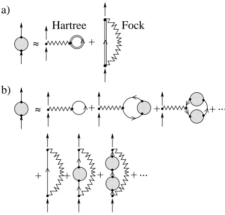
conve-nient approximations can be derived from the perturba-tive expansion over the e-p coupling strength16,24,25,28,34_.

In this work we consider the SCBA where only the Hartree and Fock diagrams of the perturbative expansion are retained (see figure 2). This is equivalent to evaluat-ing the first order diagrams at the interactevaluat-ing electronic Green function. Thus the phonon self-energy reads

Σph(ω) = ΣF(ω) + ΣH, (15)

where the retarded Hartree (H) and Fock (F) contribu-tions to the self-energies are respectively28,35

ΣH _{= i}X

λ

4 Ωλ

Z ∞

−∞

dω′

2πM

λ_Tr[G<

M(ω′)Mλ],(16)

ΣF(ω) = X

λ

" 1 2[Σ

>

λ(ω)−Σ < λ(ω)]

−₂iHω′{Σ>_λ(ω′)−Σ<_λ(ω′)}(ω) #

. (17)

In equation (17)Hω′ is the Hilbert transform

Hx{f(x)}(y) = 1

πP Z ∞

−∞

dxf(x)

x−y, (18) andP stands for the principal part of the integral. The

000 000 000 000 000 000

111 111 111 111 111 111

00 00

11 11

00 00

11 11

000 000 000 000 000 000

111 111 111 111 111 111 000 000 000 000 000 000

111 111 111 111 111 111

0 0

1 1

0000 0000 0000 0000 0000 0000

1111 1111 1111 1111 1111 1111 0000

0000 0000 0000 0000 0000 0000

1111 1111 1111 1111 1111 1111 1111

00

11

+

+

+

+

~

~

+

+

+

...

~

~

+

...

b)

a)

Hartree

Fock

000 000 000 000 000 000 000

111 111 111 111 111 111 111

000 000 000 000 000 000 000

111 111 111 111 111 111 111 000 000 000 000 000 000 000

111 111 111 111 111 111 111

FIG. 2: Diagrammatic representation of the Hartree-Fock ap-proximation. (a) the self-consistent proper self-energy (the shaded circle) is obtained from the first-order Hartree-Fock di-agrams evaluated using the interacting Green’s function (dou-ble line). This is equivalent to re-summing all the diagrams36

in (b).

phonon energy and e-p coupling matrix for a particular mode λ are respectively Ωλ and Mλ. Finally the e-p

lesser and greater self-energy are given by

ΣF≶(ω) = X

λ

Σ≶_λ(ω), (19)

Σ≶λ(ω) = Mλ

"

(Nλ+ 1)G≶M(ω±Ωλ)

+ NλG≶M(ω∓Ωλ)

#

which is simply a sum of the lesser self-energies over all the possible modes λ. The occupancy of each phonon mode isNλ.

We assume that the phonons are in thermal equilbrium with a bath so that for a given temperatureNλis simply

the Bose-Einstein distribution Nλ = (eΩλ/KBT −1)−1,

withKBthe Boltzman constant. From equation (20) we

note that the lesser (greater) self-energy contains con-tributions from two scattering processes: electrons with energyω−Ωλ may absorb (emit) a phonon and/or

elec-trons with energyω+ Ωλ may emit (absorb) a phonon

of energy Ωλ. When T ∼ 0, electrons may only emit

phonons since Nλ ∼ 0, i.e. no phonons are present in

the scattering region provided that the phonon lifetime is much smaller than that of the electrons. The total lesser self-energy of equation (6) must be adjusted to in-clude the phonon lesser self-energy,

Σ≶(ω) = X

α= L,R

Σα≶(ω) + Σ≶_ph(ω) (21)

and G≶_{(ω) from equation (5) are now evaluated using}

the perturbed Green function and lesser self-energy from equations (14) and (21). The general expression for the interacting (including e-p coupling) current37 _through

lead β may be written as the sum of an elastic and an inelastic contribution

Jβ(V) = J_elβ(V) +J_inelβ (V), where

Jelβ=

2e h

Z ∞

−∞

dωTr[ΓβGMΓαG†M](n

β

F−nαF) (22)

and

J_inelβ =2e h

Z ∞

−∞

dωTr "

Σ<βGMΣ>phG

†

M−Σ>βGMΣ<phG

†

M

# . (23)

III. NUMERICAL METHOD

A. Model Hamiltonian and Coupling Matrices Mλ

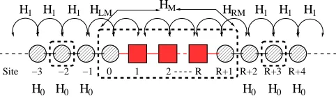
The systems under investigation are 1D linear atomic chains described by a s-orbital nearest-neighbour tight-binding model. The scattering region comprisesRatoms plus one PL (one atom) from each lead, so that it contains M =R+ 2 orbitals. Henceforth we refer to this system as RC. Furthermore, we assume that the two leads are identical. The matrices H0, H1 for a 1D tight-binding

model reduce to c-numbers:ǫL =H0andγL =H1, where

ǫL, γL are the lead onsite energy and hopping parameter

respectively. The leads’ Hamiltonians thus read

HL = ǫL

−1

X

i=−∞

c†_ici+γL

−2

X

i=−∞

[c†_ici+1+c†i+1ci],(24)

HR = ǫL

∞

X

i=R+2

c†ici+γL

∞

X

i=R+2

[c†ici+1+c†i+1ci],(25)

0000 0000 0000

1111 1111 1111

000 000 000

111 111 111

000 000 000

111 111 111

0000 0000 0000

1111 1111 1111

000 000 000

111 111 111

000 000 000

111 111 111

0000 0000 0000

1111 1111 1111

0000 0000 0000

1111 1111 1111

H1 H1

H1 H1 HLM HM HRM H1 H1

H0 H0 H0 H0 H0 H0

Site −3 −2 −1 0 1 2 R R+1 R+2 R+3 R+4

FIG. 3: Schematic diagram of the simple monatomic systems considered here. It is composed of two semi infinite leads and a scattering region. The scattering region is marked with a dashed rectangle. Inelastic scattering is effective only in the scattering region.

where{c†_i, ci}are the electronic creation and annihilation

operators at sitei. The interaction Hamiltonian between the leads and the scattering region is

HLM = γLM[c†−1c0+c†0c−1] (26) HRM = γLM[c†R+1cR+2+c†R+2cR+1], (27)

where for our setupγLM=γL.

For a 1D system the lead self-energies are analytical

ΣR

L(R)(ω) = ∆(ω)−i

Γ(ω)

2 , (28)

where

∆(ω) = Γ0

x, |x| ≤1

x−√x2_{−1 |x|>1} , (29)

Γ(ω) = −2Γ0θ(1− |x|)(

p

1−x2_{) (30)}

and Γ0=

γLM2

γL , x=

(ω−ǫL)

2γL .

Finally e-p interaction is included into the scattering re-gion in the form of an SSH Hamiltonian29,30_{, comprising}

three terms

HM=He+Hep+Hph, (31)

with

He =

R+1

X

i=0

ǫic†ici+

X

i6=j

γij0(c†icj+c†jci), (32)

Hph =

λmax

X

λ=1

(b†_λbλ+

1

2)~ωλ, (33)

Hep =

λmax

X

λ=1

X

i6=j

Mijλ(b†λ+bλ)(c†icj+c†jci). (34)

He is the electronic Hamiltonian of the scattering

re-gion with onsite energies ǫi and the unperturbed

hop-ping parameters γ0

ij (we assume γij0 = 0 for j 6=i±1).

Hph is the non-interacting phonons Hamiltonian,

with the indexλrunning over all the modes45_{. The final}

term, Hep, is the Hamiltonian describing the e-p

inter-action within the scattering region. The details of such interaction are included in the e-p coupling matricesMλ

ij.

In order to calculate the matrices Mλ

ij and the

longi-tudinal phonon frequencies we consider a simple nearest neighbours elastic model23,24,38 _{in which}

Mijλ =αij

( ei

λ

√_m

i −

ej_λ

√_m

j

) r

~

2ωλ

. (35)

In equation (35) the orthonormal vectorseλrepresent the

ionic displacement associated to each modeλ,mi is the

mass of the atom at sitei, and the constantsαij are the

e-p coupling parameters. These latter are defined as the first order coefficient of the expansion of the tight-binding hopping parameterγij about the atomic equilibrium

po-sitions

γij =γij0 +αij(ui−uj), (36)

where ui is the displacement vector of the atom at site

i. From equation (36) it follows that αij =−αji. In

the nearest neighbour approximation the interaction is restricted to electrons moving between sites iand i±1. Finally, we note that the eigenvectorseλ are real. This

implies that the matrices Mλ

ij are real and symmetric

with non-zero matrix elements fori=i±1, so that Mλ ij

has a tri-diagonal form for longitudinal phonons. We note that, although it is possible calculate the coupling parametersαij using first-principles electronic structure

methods, here we set αij =α and α is taken as a free

parameter.

B. Numerical Integration and Self Consistency

The flowchart in figure 4 outlines the numerical pro-cedure used to calculate the interacting current Jβ_(V)

and the differential conductanceG(V). Each simulation can be partitioned into three steps. The first two consist of two self-consistent loops which calculate the phonon self-energies ΣH _{and Σ}F _{respectively. These are used in}

the third step to evaluateJβ_{(V) by using the equations}

(22) and (23).

Let us now discuss the three steps in some detail. We start by writing ΣH_{as an explicit function of the density}

matrixρ

ΣH_{(ρ) = −4}X

λ

Tr

ρM

λ

Ωλ

Mλ_{, (37)}

where we assume that all the elements of G<_M are inte-grable. ΣH _{is thus nothing but a weighted sum of the}

matricesMλ_{. This can be written in the form}

ΣH=

M

X

λ=1

rλRλ, (38)

n

rn₁, rn₂, r...n , r_Rn}

{

E

Numerical Parameters

T

H_MΣ(ωi)

L(R)

Ωλ

Mλ

System Parameters

n

c1

(ωi)

G0 G(ωi)

> <,0

(ωi) F,

Σ 0

(ωi)

Σ>< ,0 ph

(ωi) F,

Σ n >< ,n

(ωi)

Σ_ph Gn(ωi) G(ωi)

> <,n

n

c2

( )_V

J

(ωi)

G G(ωi)

> <

Converged

Hartree s−c loop

Fock s−c loop

ρ

NFp (dE)F tF

Fock: , ,

V_final

V_init, ,dV

Bias:

dE

( )_H,tH

rp1

cp1cp2

B, , , ,Poles

Hartree: _{, ,}

F

E , ,

c c−e [k ,k , m]

Initialisation

r

{ }

tH

< ?

M , M

ΣH

=0, =0,

M , M

,

?

tF

<

β

M , M

1

2

3

G(V)

V=V+dV

Outputs

FIG. 4: Scheme of our numerical procedure for self-consistency.

where the ratio matricesRλ _{and their weighting}

coeffi-cientsrλ are given by

Rλ = |γ

0 |min |Mλ_|

maxM

λ_{. (39)}

rλ = −4|M λ_|

max

Ωλ_|γ0_| min

M−1

X

i=1

Rλi,i+1(ρi,i+1+ρi+1,i), (40)

For a given modeλ, the largest matrix element of the matrixMλ_{is denoted as|M}λ_|

max. |γ0|minis the smallest

among the hopping parameters of the unperturbed sys-tem (no e-p coupling), which, by construction, is equal to|Rλ_|

max. The matricesRλare independent of the e-p

couplingαand simply reflect the symmetry of the specific phonon mode considered. Thus rλ measures the

maxi-mum fractional modification of the elements γ0

ij in the

electronic Hamiltonian as the result of e-p coupling. The first self-consistent loop of figure 4 begins by choosing initial values for the weighting coefficients,

{rλ}init = {r10, r20, ..., r0R}, which are used to construct

{rλ} andρare varied until the convergence condition

cn1 =

X

λ

|rn λ−r

n−1

λ |

|rn−1

λ |

!

< tH (41)

is met for the chosen tolerance tH. The density matrix

ρis obtained by integrating G< as in equation (10). In order to perform this integral we first take ΣF_{= 0 under}

the assumption that this has little effect of the conver-gence ofρ(first self-consistent loop). Following previous works27,39_{we write ρ=ρ}

eq+ρV, where

ρeq = −1

π Z ∞

−∞

dωIm[GM]nLF, (42)

and

ρV= 1

2π Z ∞

−∞

dω GMΓRG†_M(nRF−nLF). (43)

At equilibrium (µL=µR=µ) one hasρ=ρeq.

EB

E_F−V/2 E_F+V/2

n_F n_F

E_F−V/2

(R) (L)

cp₁ cp

2

Poles rp

1

[ ]ω Re

[ ]ω Im

[ ]ω Re 1

a) b)

FIG. 5: Schematic representation of the integrals in equations (43) and (42) respectively. In a) the integration ofρVis bound

betweenEF+eV /2 andEF−eV /2 by the Fermi functions.

rp1 is the number of points of the real axis energy grid. For ρeq in b) the number of grid points along the circular path

(cp1) and the path in the complex plane parallel to the real

axis (cp2) must be chosen, as well as the poles in the Fermi

functions.

As shown in figure 5a, the integral ofρV (Eq. (43)) is

along the real axis and it is bound between the chemical potentialsµLandµR. This is carried out over a numerical

grid of sufficient fineness (dE)H. The calculation of ρeq

involves an unbound integral. This is performed over a coarse grid in the complex plane using a contour integral method40_{, since G}

M is analytical41 and smooth in the

imaginary energy plane. As shown in figure 5b a number of numerical parameters must be chosen. First the lower limit of integration EB must lie below the lowest lying

molecular states and below the lowest electrode bands. Secondly, the poles of the Fermi functions (Matsubara frequencies) which lie within the contour must be taken into account. The integration is then performed by using Gaussian quadrature42 _.

The second self-consistent loop begins by calculating

{G0

M, G≷,0}using equation (14), where the converged ΣH

from the first loop is used and ΣF_{= 0. We then proceed}

to iterate{ΣF_,Σ≷

ph} and{GM, G≷} until a second

con-vergence condition is met

cn2 =

1 NF

p

Max (

|[GnM(ωi)−GnM−1(ωi)]|

)

< tF.(44)

Note that the condition is over the largest of the ma-trix elements and runs over theNF

p energy points ωi of

the entire grid. Note also that the tolerance used, tF,

is in general different to that used for the Hartree term. The Hilbert transform required for calculating the imag-inary part of ΣF _{(eq. (17)) is done by using a}

convo-lution method combined with a fast Fourier transform algorithm24_{. In order to avoid end-point corrections we}

choose a grid of sufficient range while the grid fineness (dE)F must be sufficiently fine to resolve phononic

fea-tures which lie in the meV range.

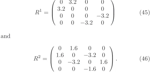
Table I shows the numerical and system parameters used in our simulations. The parameters for the H2-Pt

junctions are identical to those used by Jean11_{within the}

EST treatment of phonons. This set produces the same unperturbed G(0) ∼ .97G0. The spring constants and

masses are chosen to give longitudinal phonon modes of energies 63 meV (CM mode) and 432 meV respectively while the ratio matrices for these two modes are

R1= 

 

0 3.2 0 0 3.2 0 0 0 0 0 0 −3.2 0 0 −3.2 0





 (45)

and

R2= 

 

0 1.6 0 0 1.6 0 −3.2 0 0 −3.2 0 1.6 0 0 −1.6 0





. (46)

The e-p couplingαremains a free parameter.

The parameters for the Au RC’s match closely those used by Frederiksen of24_{. The atoms in the leads are}

chosen as identical to the atoms in the scattering region, thus that a single onsite energy and hopping parameter characterise the electronic Hamiltonian. These parame-ters and the equilibrium potentialµeqare chosen so that

the differential conductance for the unperturbed system isG0= 2e2/h(perfect transmission).

IV. RESULTS: H2-Pt JUNCTIONS

A. self-consistent simulations

System parameter H2−Pt Au RC

Symbol Value Value Units

EF 0.00 0.00 eV

ǫM (molecule) -6.0 0.0 eV ǫL (leads) 0.00 -1.00 eV

γL(leads) 5 -1.00 eV

γM(molecule) 6.0 -1.00 eV

γLM 3.2 -1.00 eV

T 4.0 4.0 K

m(atomic mass) 1 197 amu

Kc 21.82 2.00 eV/˚A2

Kc−e 0.91 1.00 eV/˚A2

Numerical parameter Value Value Units [Vini, Vfinal] (Bias Range) [0,200] [0,31] meV

Number of Bias points 250 120 – (dE)F(Fock) 0.1 0.1 meV NF

p (Fock) 12600 12600 –

rp1, (Hartree) 4000 4000 –

(dE)H(Hartree) .1061 .0215 meV

cp1(Hartree) 400 200 –

cp2(Hartree) 400 200 –

EB(Hartree) -28.0 -5.0 eV

Poles (Hartree) 80 80 –

tF(Tolerance) 9.10−8 9.10−8 eV−1 tH(Tolerance) 1.10−8 1.10−6 –

TABLE I: Parameters used to simulate the H2-Pt junctions

and Au RC’s. The parameter Kc is to the spring constant

between the atoms in the chain, while Kc−e is to the spring

constant between the molecule and the electrodes. The Fock grid and real Hartree grid are symmetric aboutEF.

processes involving the emission of phonons with ener-gies Ω ≈eVthr. We quantify this effect by defining the

conductance drop (in units ofG0)

∆thr=G(0)−G(Vthr). (47)

Numerical simulations are carried out in two differ-ent ways. First, we follow the exact numerical pro-cedure of figure 4 (“full SCBA”), but we run simula-tions starting with different initial condisimula-tions, namely

{rλ}init= + 0.003125 and {rλ}init= −0.003125. In

figure 6a ∆thr is plotted versus α demonstrating good

agreement between the full SCBA and EST for low α. However, the two methods disagree for α beyond αcrit∼1.8 eV/˚A. ∆thr peaks sharply above αcrit,

be-yond which it becomes dependent on the initial condi-tion{rλ}init. This last situation is shown in figure 6c for

α= 2.0 eV/˚A where two differentG(V) curves are pre-dicted for different {rλ}init and a low-bias conductance

of 0.0125G0 is observed in stark disagreement with the

unperturbed value of∼0.97G0.

Since the Hartree self-consistent loop is performed

be-1.6 1.7 1.8 1.9 2 2.1 2.2 α [eV/Å]

-0.05 0 0.05 0.1 0.15 0.2

∆thr

[G

0

]

{r_λ}_init= -0.003125 {r_λ}_init= +0.003125 EST

0 0.5 1 1.5 2 2.5 3 3.5 4 4.5 5 α [eV/Å]

0 0.05 0.1

∆thr

[G

0

]

EST SCBA (ΣH = 0)

0 0.025 0.05 0.075 0.1

V [eV]

0.005 0.01 0.015 0.02 0.025

G(V) [G

0

]

{r_λ}_init = -0.003125 {r_λ}_init = +0.003125

0 0.05 0.1

V [eV]

0.945 0.95 0.955 0.96 0.965 0.97 0.975

G(V) [G

0

]

EST SCBA (ΣH

= 0) a)

c)

b)

d)

α = 2.00 eV/Å α = 2.00 eV/Å

FIG. 6: Differential conductance and conductance drop at threshold for the H2-Pt junctions -Vthris taken at 68.5 meV.

Results obtained using the full SCBA are given for the dif-ferent initial conditions (panels a and c). In panels b) and d) we also show results obtained by setting ΣH _{= 0. In this}

second case ∆thr andG(V) agree well with the EST11(EST)

up toα≈4.0 eV/˚A. The full SCBA disagrees with the EST at a considerably lowerα≈1.8 eV/˚A. Above such a coupling strengthG(V) depends on the initial conditions.

fore the Fock one, the dependence on the initial condi-tions suggests that ΣH may be responsible for the be-haviour observed for α > αcrit. Stronger evidence to

support this hypothesis is provided in figures 6b and 6d where the results for our second set of simulations in which ΣH _{is set to zero, are presented (“partial SCBA“).}

Figure 6b shows good agreement between the partial SCBA and the EST to the much higher coupling of α∼4.0 eV/˚A. Moreover there is no evidence of anyαcrit.

This is confirmed by theG(V) curve obtained forα= 2.0 eV/˚A and presented in figure 6d.

B. Contribution from the individual modes

We now analyze the origin the breakdown of the full SCBA. ForV ≪Vthrthe inelastic currentJinelis strongly

suppressed by Pauli exclusion principle. At low temper-ature (T=4.0 K) we can approximate the Fermi distribu-tions inJelby step functions to obtain

Jβ_{(V) ≃} 2e

h Z µR

µL

T(ω)dω .

We can now easily probe the contribution of the Hartree term to the conductance by considering the test Green function

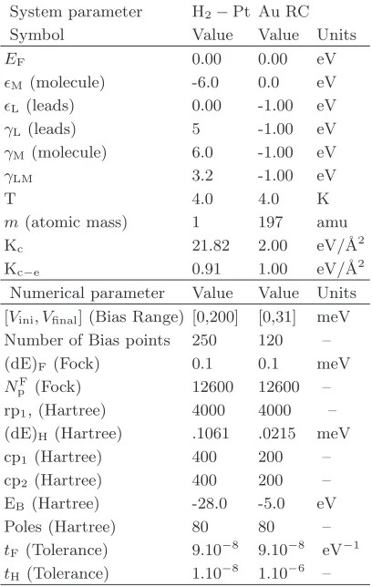
This is used to evaluate the transmission coefficient at V = 0 and it is useful to understand the influence of the individual modesλover the transmission. In figure 7 we show T(ω) as a function of rλ for the two longitudinal

modes available in the H2-Pt system (see figure 8). In

the case of the rigid translational mode (λ= 1 and fig-ure 7a)T(ω) is reduced in the region aroundEF as |r1|

increases. However the general shape ofT(ω) is little af-fected. This is somehow expected from the shape of the matrixR1_{(eq. (45)), which indicates that mode 1 causes}

simply a change in the hopping parameters γ0

12 andγ340

connecting the molecule to the leads. Importantly when γ0

12is increased,γ340 is reduced by the same amount and

vice-versa. Moreover there is a symmetryr1→ −r1.

-10 -5 0 5 10

ω -E_F [eV]

0 0.2 0.4 0.6 0.8

T(

ω

) [G

0

]

r₁

r₂

b)

a)

r

2 = -0.4|γ

0 min| r

2 = 0

r

2 = +0.4|γ

0 min| 0

0.2 0.4 0.6 0.8

T(

ω

) [G

0

] r1 = 0

r₁ = 0.2|γ0_min|

r₁ = 0.4|γ0_min|

FIG. 7: Transmission coefficients calculated using the Green function Gλ

M of Eq. (48) for λ= 1 (a) and λ = 2 (b). The

matricesR1_andR2_{are fixed and a range of values forr}

λhas

been chosen.

The results for the symmetric mode λ = 2 are pre-sented in figure 7b. This time the peak in transmission is shifted in energy either to the left or to the right de-pending on the sign ofr2. When shifted to the left, the

peak is broadened while a shift to the right narrows it. In either case the transmission aroundEFis reduced.

0000000 0000000 0000000 0000000 0000000 0000000 0000000

1111111 1111111 1111111 1111111 1111111 1111111 1111111

0000000 0000000 0000000 0000000 0000000 0000000 0000000 0000000

1111111 1111111 1111111 1111111 1111111 1111111 1111111 1111111

00000000 00000000 00000000 00000000 00000000 00000000 00000000

11111111 11111111 11111111 11111111 11111111 11111111 11111111

00000000 00000000 00000000 00000000 00000000 00000000 00000000 00000000

11111111 11111111 11111111 11111111 11111111 11111111 11111111 11111111

0000 0000 0000 0000 0000 0000

1111 1111 1111 1111 1111 111100001111

0000 0000 0000 0000 0000 0000

1111 1111 1111 1111 1111 1111

0000 0000 0000 0000 0000 0000

1111 1111 1111 1111 1111 1111 0000

1111

Mode 2

0000 0000 0000 0000 0000

1111 1111 1111 1111 1111 1111

0000 0000 0000 0000 0000 0000

1111 1111 1111 1111 1111 1111 00000 11111

0000 0000 0000 0000 0000 0000

1111 1111 1111 1111 1111 1111 00000 11111

0000 0000 0000 0000 0000 0000

1111 1111 1111 1111 1111 1111

0000 0000 0000 0000 0000 0000

1111 1111 1111 1111 1111 1111

Mode 1

FIG. 8: The longitudinal vibration modes of H2-Pt junctions.

Theλ= 1 mode of energy 63 meV is the rigid translational of the H2 centre of mass, while theλ= 2 mode is the symmetric

mode of energy 432 meV. The atoms of the leads are fixed.

From the figures 6c, 7a, and 7b one can conclude that the deviation of the zero bias differential conductance from its unperturbed (no e-p interaction) value is a mea-sure of the magnitude of the e-p perturbation. We define

this deviation as

∆G=G0−G(0)∼=G0−T(EF), (49)

where the last equality is valid forT →0. Figures 9a and 9b show the estimated deviation (in units ofG0) versus

the weighting coefficientsrλ. The maximum deviation,

∆G = 1, occurs when the chain actually breaks as for mode 1 andr1 = 1. As expected, the curve in figure 9a

for mode 1 is symmetric about 0 while figure 9b for mode 2 is not.

-6 -4 -2 0 2 4 6

r_λ [arb. units] 0

0.2 0.4 0.6 0.8

∆

G [G

0

]

a)

b)

λ = 1

λ = 2

mode 2 0

0.2 0.4 0.6 0.8 1

∆

G [G

0

]

mode 1

-0.2 -0.1 0 0.1 0.2 r_λ [arb. units] 0

0.05 0.1 0.15 0.2

∆

G [G

0

]

-0.2 -0.1 0 0.1 0.2 r_λ [arb. units] 0

0.05 0.1 0.15 0.2

∆

G [G

0

]

FIG. 9: Estimate of the deviation ∆Gcaused by an individual modeλas a function of rλ. The insets shows the region of

small perturbation.

C. Discussion of the self-consistent results

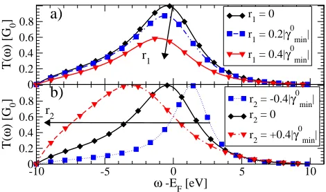
We finally re-analyze our self-consistent results in the light of the discussion in the previous section. Figure 10a and 10b show the self-consistently calculatedrλ as a

function ofαforV = 0, while figure 10c shows ∆Gas de-fined in equation (49). The critical pointαcrit∼1.8 eV/˚A

marks a sharp transition in the behaviour of the weight-ing coefficients. This is evident in the abrupt change of magnitude and behaviour of ∆G (in figure 10c). In fact while for α < αcrit the full SCBA agrees well with

the EST, the two differ sharply as soon as α > αcrit.

Going into more details we note that r1 is identically

zero (∼10−14_{) forα < α}

crit, while r2 is small and

neg-ative. Importantly both r1 and r2 are independent of {rλ}init. By contrast, forα > αcrit,r2 remains

indepen-dent of {rλ}init but this is not the case for r1. In fact

we obtain a strong dependence over the initial condi-tions with positive (negative)r1 for positive (negative) {rλ}init. Importantly none of these features are found in

the case when we neglect the Hartree self-energy. Since|r1|is two orders of magnitude larger than|r2|,

-4 -2 0 2 4 6

r1

[arb. units]

mode 1 ( {r_λ}_init > 0) mode 1 ( {r_λ}_init < 0)

0 0.01 0.02 0.03 0.04

r2

[arb. units]

mode 2 ( {r_λ}_init > 0) mode 2 ( {r_λ}_init < 0)

0 0.5 1 1.5 2 2.5 3

α [eV/Å] 0

0.2 0.4 0.6 0.8

∆

G [G

0

]

a)

b)

c)

FIG. 10: Converged self-consistent values ofrλand deviation

∆G (Eq. (49)) as a function of the e-p coupling strengthαfor

V = 0. A transition is apparent atα= 1.865±0.005 eV/˚A for the full SCBA. Panels a) and b) show respectivelyr1and r2 for the full SCBA for different initial conditions, while in

c) results for the partial SCBA and EST are also included.

varies roughly linearly with αaboveαcrit, therefore the

self-consistent ∆G follows the estimated curve of figure 9a in this region ofα. The magnitude ofr1 forα > αcrit

suggests that the interaction with phonons becomes a strong perturbation of the electronic system. We define the regionα < αcritas the weak coupling regime and the

regionα > αcrit as the strong coupling regime.

Figure 10 adequately explains the causes of the mas-sive reduction of G(V) with respect to its unperturbed value observed in figure 6c atV = 0. Notably, as figure 6a shows, ∆thr calculated with the full SCBA starts

de-viating from the EST result forα≃1.75 eV/˚A, i.e. at a value lower thatαcrit= 1.865±0.005 eV/˚A calculated for

V = 0. This seems to suggest that the critical value of αfor the breakdown of the full SCBA somehow depends on the bias. Moreover at finite bias αcrit is

character-ized by a peak in ∆thr(α) for positive{rλ}init and by a

discontinuity for negative{rλ}init (see figure 6a).

In order to explore the onset of the breakdown of the SCBA at finite bias in figure 11a we present G(V) for α= 1.84 eV/˚A i.e. just below the zero-bias critical value. In addition, in figure 11b we plot the dominant coefficient r1 for a small range of α about αcrit at three different

bias, V = 0, V = 0.1 and V = 0.2 Volt. A clear result from figure 11a is that the presence of ΣH _introduces

a reduction of G(V) with bias not present at V = 0. For α < αcrit figure 11b shows that |r1| is a function of

bias whose value increases as the bias increases. The difference between r1 atV = 0 and at finiteV explains

the deviation belowαcrit and also the origin of the peak

above it.

The discontinuity in ∆thrfor{rλ}init>0 of figure 6a is

explained by the discontinuities observed inr1(Fig. 11b)

and in the currentJβ_{(V) (Fig. 11c). In fact atV = 0,}

1.9 2 2.1 2.2

α [eV/Å]

0.5 1 1.5 2 2.5 3

|r1

| [arb. units]

V = 0.2 eV {r_λ}_init = -0.003125 V = 0.2 eV {r_λ}init = -0.003125

1.78 1.8 1.82 1.84 1.86 1.88

α [eV/Å]

-0.4 -0.2 0 0.2 0.4 0.6 0.8

r1

[arb. units]

V =0.1 eV V =0.2 eV

V = 0 {r_λ}_init = +0.003125 V = 0 {r_λ}_init = -0.003125

0 0.05 0.1 0.15

V [eV] 0

0.2 0.4 0.6 0.8 1

J

β [µ

A]

{r_λ}init = -0.003125

{r_λ}_init =+0.003125

0 0.05 0.1 0.15

V [eV] 0.825

0.85 0.875 0.9 0.925 0.95 0.975 1

G [G

0

]

SCBA SCBA (ΣH = 0) a)

c)

b)

d)

α = 1.84 eV/ Å

α = 1.885 eV/ Å

FIG. 11: Behaviour of the SCBA in the region above and be-low the zero-biasαcrit. Forα < αcrit,G(V) for the full and

partial SCBA are compared in panel a), showing that the con-tribution arising from ΣH _{is bias-dependent. For α > α}

crit, Jβ _{calculated with the full SCBA is presented in c) for two}

different initial conditions. In panel b) the functional depen-dence of the weighting coefficientr1upon bias is investigated

for a range of coupling strengths and bias. Finally, in panel d) we show the magnitude|r1|obtained from two full SCBA simulations with different initial conditions andα > αcrit.

r1 is single valued as long as α < αcrit. For α > αcrit

instead r1(α) has a parabolic shape symmetric about

r1= 0: the{rλ}init<0 solution traces out the lower arm

of the parabola and the{rλ}init>0 solution follows the

upper arm as α increases. For V > 0, it is seen that the two solutions forr1 are identical, and asymptotically

approach the lower arm of the V = 0 curve from be-low forα > αcrit. However, asαis further increased the {rλ}init>0 solution jumps discontinuously above zero

and then asymptotically approaches the upper arm, again from below.

The discontinuity in r1(α, V) is determined by both

the bias and the initial conditions. Generally, it is found that such discontinuity occurs for lower bias first; r1 jumps discontinuously for V = 0.1 Volt before it

does for V = 0.2 Volt. This explains the behaviour of the{rλ}init= +.003125 solution forJβ(V) in figure 11c

which leads to a peak in its derivative (the conductance G(V)) and explains the discontinuity of ∆thr.

We note that after the discontinuity inr1 for V > 0,

the two solutions are no longer symmetric aboutr1= 0

and do not converge to the V = 0 solutions of either arm untilα≈3.0 eV/˚A. This is highlighted in figure 11d where |r1| for the two solutions is plotted in a range of

α just above αcrit at V = 0.2 Volt. Such differences

explain why ∆thr is not independent of the initial

-30 -20 -10 0 10 20 30 V [meV] 0.99 0.9925 0.995 0.9975 1

G (V) [G

0

]

0 0.2 0.4 0.6 0.8 1

α [eV/Å]

-0.010 0.01 0.02 0.03 0.04 0.05 ∆ G [G 0 ]

0.8 0.9 1 1.1

α [eV/Å]

0 0.2 0.4 0.6 0.8 1 ∆ G [G 0 ]

{r_λ}

init = - 3

{r_λ}

init = + 3

α = 0.8 eV/Å

a)

b)

FIG. 12: G(V) for the 4C illustrating the onset of in-elastic processes at threshhold voltages. These are associ-ated to the symmetric modes of energy Ω2 = 6.5 meV and

Ω4 = 12.2 meV. The rigid and anti-symmetric modes of

en-ergies respectively Ω1 = 3.1 meV and Ω3 = 9.8 meV have

no effect for chains comprising an even number of atoms. No overall shift in G(V) is observed asα lies below the critical coupling αcrit which is clearly determined from the inset in

panel b.

We make a final comment about the discontinuities seen in figure 11a. The value ofαat which these occur is dependent on the initial conditions as mentioned already. Thus for a particular{rλ}init it may be possible to reach

the upper solution atαcrit for all bias, so that r1 has a

parabolic shape for bias while being asymmetric about 0. We have not observed this and regard αcrit as uniquely

defined forV = 0 only.

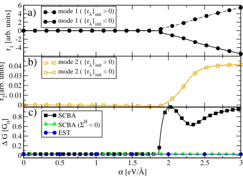
V. RESULTS:Au Chains

By using the procedure outlined in section III and the parameters of table I, the full SCBA is used to calculate the transport of the Au RC’s. In general we observe a behaviour similiar to that of the H2-Pt system. For

3C, 4C, 5C, and 6C a weak coupling regime is identified where the shift ∆G and the weighting coefficients are zero. A critical coupling strength αcrit for V = 0 was

discovered for each of the chains investigated with values αcrit≈0.85,0.9,0.82,0.83 eV/˚A respectively for 3C, 4C,

5C, and 6C. For weak coupling ∆Gmatches closely the values calculated in previous works24,35_{. As an example,}

in figure 12 we presentG(V) and ∆G(α) for 4C. It is seen that the modes symmetric with respect to the centre of the scattering region (even numbered) induce drops in G(V) at threshhold voltages corresponding to the energy of the modes. In general, only the symmetric modes are active in RC’s containing an even number of atoms and conversely the rigid and anti-symmetric modes are active

0000000 0000000 0000000 0000000 0000000 0000000 0000000 0000000 1111111 1111111 1111111 1111111 1111111 1111111 1111111 1111111 00000000 00000000 00000000 00000000 00000000 00000000 00000000 00000000 11111111 11111111 11111111 11111111 11111111 11111111 11111111 11111111 0000000 0000000 0000000 0000000 0000000 0000000 0000000 0000000 1111111 1111111 1111111 1111111 1111111 1111111 1111111 1111111 0000000 0000000 0000000 0000000 0000000 0000000 0000000 0000000 1111111 1111111 1111111 1111111 1111111 1111111 1111111 1111111 0000000 0000000 0000000 0000000 0000000 0000000 0000000 0000000 1111111 1111111 1111111 1111111 1111111 1111111 1111111 1111111 0000000 0000000 0000000 0000000 0000000 0000000 0000000 0000000 1111111 1111111 1111111 1111111 1111111 1111111 1111111 1111111 0000000 0000000 0000000 0000000 0000000 0000000 0000000 0000000 1111111 1111111 1111111 1111111 1111111 1111111 1111111 1111111 00000000 00000000 00000000 00000000 00000000 00000000 00000000 00000000 11111111 11111111 11111111 11111111 11111111 11111111 11111111 11111111 0000 0000 0000 0000 0000 0000 1111 1111 1111 1111 1111 1111 0000 0000 0000 0000 0000 0000 1111 1111 1111 1111 1111 1111 000 000 000 000 000 111 111 111 111 111 0000 0000 0000 0000 0000 0000 1111 1111 1111 1111 1111 1111 Mode 3(A) 0000 0000 0000 0000 0000 0000 1111 1111 1111 1111 1111 1111 0000 1111 0000 0000 0000 0000 0000 0000 1111 1111 1111 1111 1111 1111 00000 11111 0000 0000 0000 0000 0000 0000 1111 1111 1111 1111 1111 1111 0000 1111 0000 0000 0000 0000 0000 0000 1111 1111 1111 1111 1111 1111 00000 11111 0000 0000 0000 0000 0000 0000 1111 1111 1111 1111 1111 1111 0000 0000 0000 0000 0000 0000 1111 1111 1111 1111 1111 1111 Mode 1(R) 0000 0000 0000 0000 0000 0000 1111 1111 1111 1111 1111 1111 0000 1111 0000 0000 0000 0000 0000 0000 1111 1111 1111 1111 1111 1111 0000 1111 000 000 000 000 000 111 111 111 111 111 0000 1111 0000 0000 0000 0000 0000 0000 1111 1111 1111 1111 1111 1111 0000 1111 0000 0000 0000 0000 0000 0000 1111 1111 1111 1111 1111 1111 Mode 2(S) 0000 0000 0000 0000 0000 0000 1111 1111 1111 1111 1111 1111 0000 0000 0000 0000 0000 0000 1111 1111 1111 1111 1111 1111 00000 11111 0000 0000 0000 0000 0000 0000 1111 1111 1111 1111 1111 1111 00000 11111 0000 0000 0000 0000 0000 0000 1111 1111 1111 1111 1111 1111 00000 11111 0000 0000 0000 0000 0000 0000 1111 1111 1111 1111 1111 1111 0000 1111 0000 0000 0000 0000 0000 0000 1111 1111 1111 1111 1111 1111 Mode 4(S)

FIG. 13: Vibration modes of Au 4C. Modes 2 and 4 are sym-metric modes (S) about the centre of the scattering region. Mode 1 is the rigid translational mode (R) while mode 3 is anti-symmetric (A). For all chains considered, the mass of the lead atoms are taken sufficiently larger than that of the chain atoms so that they do not vibrate.

1 10 100 1000 10000

n -0.1 -0.05 0 0.05 0.1 r 4 [arb. units]

{r_λ}_init = 0 eV {r_λ}_init = +- 0.02 {r_λ}_init = +- 0.04 {r_λ}_init = +- 0.06 {r_λ}_init = +- 0.08

α = 0.902 eV/Å

FIG. 14: Test of the convergence of the weighting coefficient r4 for the 4C andα > αcritusing a range {rλ}init where n is

the number of iterations. Results for the calculations with positive starting values are indicated with dashed lines while those with negative initial values are shown with solid lines. A single negative and positive solution for the converged r4is

found.

for an odd RC.

The transition from weak to strong coupling can be ap-preciated for the 4C by looking at the inset of figure 12b, where forα > αcrittwo different initial conditions lead to

two different ∆G. The 6C shows the same behaviour of the 4C, while the 3C and 5C show a single curve for ∆G due to the symmetry of the weighting coefficients in the strong regime. Beyondαcrit, for all the RC’s simulated

G(V) is reduced to zero asαincreased and the shift ∆G rises toG0 .

Finally we want to investigate further the existence of multiple solutions depending on the initial conditions in the self-consistent loops. As an example of how conver-gence is achieved in figure 14 we show the coefficientr4

as a function of the iteration numbernfor the 4C plotted for a single biasV = 0.02 Volt and coupling 0.902 eV/˚A (α > αcrit). A number of simulations were run with

dif-ferent initial conditions. The figure indicates the exis-tence of two stable minima: simulations which start at

{rλ}init>0 (dashed lines) converge to the same positive

final value, while simulations initialised with{rλ}init<0

converge to the samer6<0 value. We note that the

min-ima are not symmetric aboutr6= 0. The solutionrλ= 0

10 100 1000 10000 n

-0.25 -0.2 -0.15 -0.1 -0.05 0

r6

[arb units]

α = 0.902 eV/Å

EB = -0.5 eV EB = -1.0 eV EB = -1.5 eV EB = -2.0 eV EB = -2.5 eV EB = -3.0 eV EB = -3.5 eV

FIG. 15: Convergence test. The zero-biasr6is plotted versus

the iteration number n for {rλ}init=−0.09 and α > αcrit.

Here the lower bound for the integration of the charge density

ρ, EB, is varied. The lower bandedge of the leads lies at -2 eV. Clearly when EB≥ −2 eVr6 does not converge fully,

i.e. it depends on EB.

strong coupling regime.

In figure 15 r6 is plotted versus the number of

itera-tionsnforα > αcrit. This time we run different

simula-tions in which the lower bound of the energy integration grid, EB, is changed. In particular we explore situations where EB is not below the lower band-edge of the leads, that for our choice of parameters lies at -2 eV (see table I). The figure indicates that if EB≥ −1 eVr6 converges

to zero so that the sixth mode gives no contribution to ΣH_{. For −2≤EB<−1 r}

6 is nonzero, however the

con-verged value differs for EB= -1.5 eV and EB= -2.0 eV, i.e. it is sensitive on the grid lower bound. Finally for EB<−2.0 eV the bands of the leads are entirely included in the integral and r6 converges to a value of

approxi-mately −0.25 eV which is independent of our choice of EB. From this simple analysis it appears that cutting the integration grid can result in the erroneous suppression of the Hartree self-energy, i.e. in a drastic underestimate of its contribution. This produces a fortuitous suppres-sion of the SCBA breakdown, since the agreement be-tween SCBA and EST is usually improved when ΣH _is

neglected.

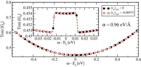
Finally we test the robustness of our integration method. Figure 16 shows the transmission coefficients T(ω) for a 6C at a bias of V = 1 mV where only the sixth mode is considered. We run two simulations. In the first case, the full SCBA is used with the numer-ical parameters taken from table I and initial condi-tion {r6}init=−0.00975. In the second case, the

in-tegration method outlined in section III B is replaced by Simpson’s rule along the real axis. The integra-tion range used is [-3.093,0.1] eV with a grid fineness (dE)H= 2.129×10−5 eV. The Hartree self-consistent

loop is started with {r6}init= 0.0 and finished when

cn

1<tH= 10−12(this tolerance was also used in the first

case). All other parameters of the calculations are iden-tical in the two cases. The figure shows that the two numerical methods produce the same T(ω), specifically in the range of applied bias shown in the inset.

-0.4 -0.2 0 0.2 0.4 0.6

ω - E_f [eV] 0.5

0.6 0.7 0.8

T(

ω

) [G

0

]

{r₆}_init = 0 {r₆}_init = -0.00975

-0.03 -0.02 -0.01 0 0.01 0.02 0.03

ω - E_f [eV] 0.45

0.451 0.452 0.453 0.454 0.455

T(

ω

) [G

0

]

α = 0.96 eV/Å

FIG. 16: T(ω) for a 6C simulation where only the sixth mode of energy Ω6= 12.6 meV is included. The curves

show results obtained when ΣH_{is calculated using the}

Simp-son’s rule ({r6}init= 0 in the legend) or the contour method ({r6}init=−0.00975 in the legend).

VI. CONCLUSIONS

By using a simple 1D tight binding model we have investigated the breakdown of the SCBA as a function of the e-p coupling strengthα. We have identified two regimes. In the weak coupling regime there is a unique solution for both ΣH _{and Σ}F_{, independently of the}

ini-tial conditions. In particular the Hartree self-energy is small and has little effect on the final conductance. In this weak coupling regime the characteristic conductance drops at voltages corresponding to the various phonon en-ergies compare well with those calculated with the EST method.

As the coupling parameterαis increased beyond some critical value αcrit a sharp transition to the strong

cou-pling regime occurs. In this limit the self-consistent ΣH

becomes unstable with respect to the initial conditions and exhibits multiple values for the same voltage. This results in a conductance that sharply deviates from that obtained with the exact EST. Such a sharp transition suggests a breakdown of the SCBA, indicating that the electron-phonon interaction cannot be treated perturba-tively for α > αcrit. Interestingly such a breakdown

is suppressed when the Hartree self-energy is neglected completely from the calculation, as routinely done in practice. Our results however set a warning to quantita-tive calculations based on e-p parameters extracted from density functional theory. For these, no information is available on whether or not the obtained e-p coupling strength is either below or above the critical value for the SCBA to breakdown. Therefore, strictly speaking, one rarely knows whether the SCBA is applicable.

Acknowledgments

Centre for High Performance Computing (TCHPC) and at the Irish Centre for High-End Computing (ICHEC).

∗ _{Electronic address: [email protected]}

1 _{J. I. Pascual, N. Lorente, Z. Song, H. Conrad, and H. P.}

Rust, Nature (London)423, 525 (2003).

2 _{M. Ohara, Y. Kim, and M. Kawai, Chem. Phys. Lett.426,}

357 (2006).

3 _{T. Komeda, Y. Kim, B. N. J. Persson, and H. Ueba,}

Sci-ence295, 2055 (2002).

4 _{Y. Sainoo, Y. Kim, T. Okawa, T. Komeda, H. Shigekawa,}

and M. Kawai, Phys. Rev. Lett.95, 246102 (2005).

5 _{K. W. Hipps and U. Mazur, J. Phys. Chem 97, 7803}

(1993).

6 _{B. C. Stipe, M. A. Rezaei, and W. Ho, Phys. Rev. Lett.}

82, 1724 (1999).

7 _{R. C. Jaklevic and J. Lambe, Phys. Rev. Lett 17, 1139}

(1966).

8 _{L. Cai, M. A. Cabassi, H. Yoon, O. M. Cabarcos, C. L.}

McGuiness, A. K. Flatt, D. L. Allara, J. M. Tour, and T. S. Mayer, Nano Lett5(12), 2365 (2005).

9 _{R. H. M. Smit et al, Nature (London)419, 906 (2002).}

10 _{N. Agrait, C. Untiedt, G. Rubio-Bollinger, and S. Vieira,}

Phys. Rev. Lett88, 216803 (2002).

11 _{N. Jean and S. Sanvito, Phys. Rev. B73, 094433 (2006).}

12 _{H. Ness and A. J. Fisher, Phys. Rev. Lett.83, 452 (1999).}

13 _{L. V. Keldysh, Sov. Phys. JETP20, 1018 (1965).}

14 _{A. R. Rocha et al, Nature Mat.4, 335 (2005).}

15 _{J. Rammer and H. Smith, Rev. Mod. Phys.58, 323 (1986).}

16 _{P. Danielewicz, Ann. Phys.152, 239 (1984).}

17 _{C. Caroli, R. Combescot, P. Nozieres, and D. St-James, J.}

Phys. C: Solid State Physics5, 21 (1972).

18 _{M. Magoga and C. Joachim, Phys. Rev. B57, 1820 (1998).}

19 _{M. Buttiker, Y. Imry, R. Landauer, and,S. Pinhas, Phys.}

Rev. B31, 6207 (1985).

20 _{S. Sanvito, C. J. Lambert, J. H. Jefferson, and A. M.}

Bratkovsky, Phys. Rev. B59, 11936 (1999).

21 _{J. Bonca and S. A. Trugman, Phys. Rev. Lett 75, 2566}

(1995).

22 _{K. Haule and J. Bonca, Phys. Rev. B59, 13087 (1999).}

23 _{E. G. Emberly and G. Kirczenow, Phys. Rev. B61, 5740}

(2000).

24 _{T. Frederiksen, Master’s thesis, Technical University of}

Denmark (2004).

25 _{M. Galperin and M. A. Ratner, J. Chem. Phys.121, 11965}

(2004).

26 _{E. J. McEniry, D. R. Bowler, D. Dundas, C. Horseld,}

An-drew P Sanchez, and T. N. Todorov, J. Phys.: Condens. Matter19, 196201 (2007).

27 _{A. Rocha, Ph.D. thesis, Trinity College Dublin (2007).}

28 _{S. Datta,}

Electronic transport in Mesoscopic Systems

(Cambridge University Press, 1995), 2nd ed.

29 _{W. P. Su, J. R. Schrieffer, and A. J. Heeger, Phys. Rev.}

Lett42, 1698 (1979).

30 _{W. P. Su, J. R. Schrieffer, and A. J. Heeger, Phys. Rev. B}

22, 2099 (1980).

31 _{D. Djukic et al, Phys. Rev. B71, 161402(R) (2005).}

32 _{A. R. Rocha et al, Phys. Rev. B.73, 085414 (2006).}

33 _{M. Buttiker, Phys. Rev. B33, 3020 (1986).}

34 _{H. Haug and A. P. Jauho,Quantum Kinetics in Transport}

and Optics of Semiconductors (Berlin, 1996).

35 _{T. Frederiksen, N. Lorente, M. Paulsson, and M.}

Brand-byge, arXiv:cond-mat/0702176v1 (2007).

36 _{A. Fetter and J. D. Walecka,}

Quantum Theory of Many-Particle Systems (Dover Publications,Inc.,Mineola, New York, 2003).

37 _{Y. Meir and N. S. Wingreen, Phys. Rev. lett. 68, 2512}

(1992).

38 _{C. Kittel,Introduction to Solid State Physics(John Wiley}

and Sons(New York), 1953).

39 _{M. Brandbyge, J.-L. Mozos, P. Ordejon, J. Taylor, and}

K. Stokbro, Phys. Rev. B,65, 165401 (2002).

40 _{A. R. Williams, P. J. Feibelman, and N. D. Lang, Phys.}

Rev. B26, 5433 (1982).

41 _{J. W. Brown and R. V. Churchill,Complex Variables and}

Applications, series in Science and Engineering(Mc Graw-Hill, New York, 2003).

42 _{W. H. Press, B. P. Flannery, S. A. Teukolsky, and W. T.}

Vetterling,Numerical Recipes in Fortran (Cambridge Uni-versity Press, 1992), 2nd ed.

43 _{The superscript “R” is omitted throughout the paper}

un-less necessary.

44 _{A generalisation to a non-orthogonal LCAO Hamiltonian}

is described in reference32_.

45 _{The two lowest energy modes correspond to the trivial}