Efficient non linear 3D electrical tomography reconstruction

Efficient Non-Linear 3D Electrical Tomography Reconstruction

M Molinari1, SJ Cox1, BH Blott2, GJ Daniell2

1

Department of Electronics and Computer Science

2

Department of Physics and Astronomy University of Southampton, SO17 1BJ, UK

[email protected]

ABSTRACT

Non-linear electrical tomography imaging can be performed efficiently if certain optimisations are applied to the computational reconstruction process. We present a 3D non-linear reconstruction algorithm based on a regularized conjugate gradient solver and discuss the optimisations which we incorporated to allow for an efficient and accurate reconstruction. In particular, the application of image smoothness constraints or other regularization techniques and auto-adaptive mesh refinement are highly relevant. We demonstrate the results of applying this algorithm to the reconstruction of a simulated material distribution in a cubic volume.

Keywords 3D non-linear electrical impedance tomography, optimised reconstruction algorithm, increased spatial resolution, parallel computing

1 INTRODUCTION

For many applications in industry as well as in medicine and geological research, it would be useful to know the distribution of differing materials inside a given volume. Electrical Tomography (ET) offers the possibility to reconstruct differing electrical properties of materials to give an accurate picture of their quantitative distribution. ET has numerous advantages over other methods: it is non-destructive, non-invasive and relatively inexpensive compared with competing imaging methods, such as Magnetic Resonance or X-Ray Imaging. Electrical conductivity and permittivity are reconstructed from measure-ments of the resulting potential distribution at surface electrodes after injection of a small current into the volume under investigation. ET does not require direct visual contact to substances within, for example, stirring vessels and can hence be used for applications where optical evaluation of the contents is impossible.

In process tomography, this gives information about mixing processes as well as (unwanted) cluster formations of materials in pipes. In the medical field, tomographic reconstructions can give information about lung and stomach fillings in monitoring applications as well as support the accurate location of electrical sources in the brain for Electric Encephalography (EEG) reconstructions in functional brain imaging (Committee on the Mathematics and Physics of Emerging Dynamic, 1996 and Ollikainen et al, 1996). Geological applications include detection of buried objects or historic buildings or determination of differing geological formations (Szymanski and Tsourlos, 1993).

The reconstruction of the material distribution inside the volume is a computationally very demanding process and in mathematical terms a highly ill-conditioned non-linear problem. The ill-conditioning results from the fact that one tries to obtain an image of the interior of a volume which can consist of thousands of pixels from a small set of surface measurements. Backprojection algorithms – such as used for Computed Tomography (CT) reconstruction – have proved to be inadequate for many applications, especially in the medical ET field since they lack an appropriate reconstruction and produce images of only minor quality. Though single step update reconstruction algorithms, such as the NOSER (Newton One Step Error Reconstruction, Cheney et al, 1990) proved to be better suited, they lack the full possible reconstruction of the non-linear nature of the problem.

an efficient and accurate reconstruction in section 3. Results from a simple 3D ET reconstruction problem show the achievable resolution and performance in section 4 before we draw our conclusions.

2 RECONSTRUCTION ALGORITHM

Electrical Tomography is based on the electrical properties of differing materials in a volume conductor Ω. Tomographic reconstruction tries to image the electric permeability ε and the electric conductivity distributionσwithin the domainΩ. To achieve this, a small current of normal densityjnand frequency

ω is injected into the volume conductor and the resulting potential distributionU is measured using surface electrodes. The electric field insideΩis then governed by Poisson’s equation

(

(

)

+

(

)

)

∇

(

)

=

0

⋅

∇

σ

r

ÿ

i

ωε

r

ÿ

U

r

ÿ

and the following boundary conditions

0

U

U

=

n

j

n

U

=

∂

∂

ÿ

σ

Here,U0are the measured voltages at the boundary electrodesδΩVEL, andn denotes the unit outward

normal across the current injection electrodesδΩCEL. Together with the law of conservation of charge

and the choice of a reference point for the voltages, the requirement for existence and uniqueness of a solution are satisfied (Somersalo et al, 1992). Both material parameters are functions of the position within the object,σ(r) andε(r). For reasons of clarity, we will consider imagingσonly, however, all our formulations can be extended to image the full complex material admittivityσ+iωε.

For the reconstruction of electrical conductivity, we define an objective function φ representing the error between measured electrode voltages U0 and the electrode voltages U(σ) obtained from the

computed conductivity distributionσ.

(

) (

)

(

)

ÿ

−

=

−

−

=

U

U

U

U

U

U

)

(

2

1

)

(

)

(

2

1

σ

σ

σ

φ

The number of electrodes isNL and the subscriptldenotes thel’th component of the voltage vectors.

We want to minimise φ with respect to the conductivity σ. To perform this numerically, we need to discretise the continuous problem in a way to obtain a good approximation of the real potential distribution across Ω. We employ the Finite Element method (FEM), which is a standard tool in engineering for solving elliptic partial differential equations such as the above. The potential distribu-tionU is then approximated on the finite element mesh with N nodes and we obtain the discrete nodal potential distributionUNfrom solving theforward problem represented by a system of linear equations

I

U

Y

(

σ

)

=

The nodal voltagesUNare obtained by applying the inverse of the admittance matrixY of size N x N to

the vector of injected currentsI.Y is a very sparse matrix and the solution of even large systems can be performed efficiently when certain optimisations are applied. Equation 5 is slightly extended if, for example, the Complete Electrode Model is used which takes into account the contact impedances under the electrodes and for which Somersalo et al (1992) showed uniqueness and a modelling error of less than 0.1%.

Start

Make initialσσσσguess

Compute objective functionφ

φ<φ_max?

End

Updateσσσσby∆σσσσ

Determine forward solution U(σσσσ)

yes no

Compute∆σσσσfrom

(JT_J)∆σ _{σ σ} σ _{= -J}T_(U(σσσσ_{) – U} 0)

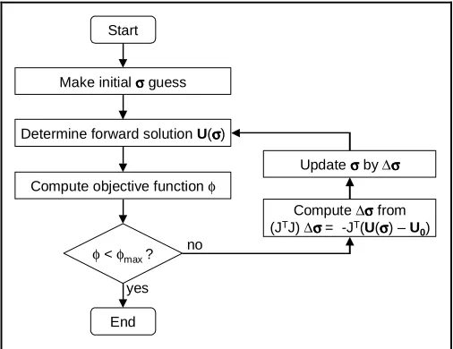
Figure 1: Outline of standard non-linear Newton-Raphson reconstruction algorithm

The resistivity update∆σfor each iteration step k of the non-linear algorithm is calculated by solving the following linear system of equations:

(

(

)

)

)

(

J

J

∆

σ

=

−

J

U

σ

−

U

whereJ is the Jacobian of the electrode potentials with respect to the elements’ conductivities and JT is the transposed ofJ.

j i ij

U

J

σ

∂

∂

=

The matrix JTJ is highly ill-conditioned in the Hadamard sense (Lamm, 1993) and the solution of this system hence requires the application of appropriate numerical techniques. Additional properties of JTJ are positive definiteness and its size is the number of elements squared (nE2).

3 OPTIMIZATIONS

We identified the requirements for an efficient reconstruction algorithm previously (Molinari et al, 2001b) as follows:

Speed

• application of sparse matrix storage schemes and solver techniques • problem-adapted mesh density

• parallelization of code

Accuracy

• usage of high-quality domain discretization • robustness with respect to noise

• minimal influence of constraints and regularization on the accuracy of the solution • suitable algorithm for the problem’s non-linear nature

Flexibility

• accurate modelling of complex 2D and 3D geometries • allow for easy application of differing boundary conditions

• possibility of FE mesh "templating" and node relocation for dynamic imaging

3.1 Finite Element Discretization

By applying the Finite Element Method (FEM), we converted the continuous problem into a problem with a finite number of unknowns. It is a known fact that the solution on the discretization tends to the true solution as the element size decreases to zero (Burnett, 1987). However, to obtain a fast algo-rithm, as few as possible elements should be used, but also as many as necessary to produce accurate solutions. It is desirable to start with a rather coarse mesh with a minimum of desired spatial resolution and then refine the discretization only where necessary.

Often, algorithms are constrained to a specific geometry (such as for example circular pipe) and the achievable performance is based on these assumptions (using cylindrical base functions). However, if the underlying geometry is of more general shape (for example the human head), the Finite Element method provides a most suitable basis for the reconstruction as it is flexible in terms of geometry and boundary conditions. We will constrain the algorithm towards the use of tetrahedral finite elements with linear base/shape functions and constant material throughout an element. This configuration allows for reduced storage as well as high computation speed.

3.2 Auto-Adaptive Mesh Refinement

If insufficient elements are used in the initial FE mesh of the problem domain Ω, the choice of discretization will affect the accuracy of the potential distribution, and also the calculation of the Jacobian in the non-linear reconstruction of the conductivities. It is therefore usual to refine the mesh globally to improve the accuracy of the solution across the whole domain. However, it is in fact only necessary to refine the mesh where the error is large: the paradox is that the exact error is only known if the exact solution is available!

We therefore use an a posteriori error estimate Σf (see Molinari et al, these proceedings) which

determines where refinement of the mesh is required. Starting with an initially rather coarse quality mesh, we refine according to this estimator and adapt the mesh to give an accurate solution. Refining of the mesh can be done in three ways:

h-refinement consists of subdividing elements into smaller elements (Burnett 1987).

p-refinement uses higher order interpolating basis functions on the elements (Zienkiewicz and Craig 1986).

r-refinement relocates the existing nodes of a mesh without adding new ones (Shepard 1985).

Efficient hybrids of these methods also exist, but can be complicated to implement. We focus on h-refinement of linear elements, which can be implemented very efficiently.p-refinement is an already commonly used improvement but produces larger matrices with increasing polynomial order. r-refinement does usually not significantly improve the solution, however, it might be useful in dynamic imaging problems, where the nodes of the mesh can follow predefined trajectories.

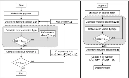
We have shown previously (Molinari et al, 2001a) that adaptive mesh refinement saves a factor of 3 in number of required elements to model theforward solution as accurately as in a globally fine mesh. This results in the speed-up of the algorithm of a factor of approximately 10 for 2D problems. Adaptive mesh refinement as part of theinverse problem based on the material gradient between elements can be used to increase the spatial resolution of the reconstructed conductivities and reduce image distortion. We have incorporated automatic mesh refinement into the reconstruction algorithm from figure 1. The algorithm allows auto-adaptive mesh refinement based on the computed a posteriori error estimate of the forward solution and uses material gradient-dependent refinement on the finally obtained solution of the inverse problem to increase resolution of material boundaries. Figure 2 shows an outline of the modified auto-adaptive algorithm.

3.3 Conjugate Gradient Solver

The conjugate gradient (CG) method is a very popular iterative method for solving large-scale systems of linear equations. It is most effective for sparse systems as its complexity scales with approximately O(nE

3/2

) in 2D and O(nE 4/3

for large problems, such as given in equation 6 for 3D imaging, methods based on the CG iterations are more efficient than other methods like LU or Cholesky decomposition.

Start

Make initialσσσσguess

Compute objective functionφ

φ<φmax?

End

Updateσσσσby∆σσσσ

Determine forward solution u(σσσσ)

Calculate error estimatesΣΣΣΣ_f(u)

Refine mesh whereΣΣΣΣflarge

||ΣΣΣΣ_f|| <Σ_f,max?

yes no

yes no

Compute∆σσσσfrom

(JT_{J)∆σ σ σ σ = -J}T_{(U(σσσσ) – U} 0)

Append

Display image

Updateσσσσby∆σσσσfrom

(JT_{J)∆σ σ σ σ = -J}T_{(U(σσσσ) – U} 0)

Determine forward solution u(σσσσ)

σσσσknown on coarse mesh

Calculate material gradientΣΣΣΣi(σσσσ)

max(ΣΣΣΣ_i) <Σ_i,max?

yes no

Refine mesh whereΣΣΣΣilarge

Figure 2: Modified reconstruction algorithm, incorporating error estimation and auto-adaptive mesh refinement for accurate forward solution (left) and material-gradient based mesh refinement step to improve image resolution (right)

As for ill-conditioned systems, the CG method often converges very well in the first iterations before noise in the singular value decomposition (SVD) components breaks down the conjugacy (Shewchuk, 1994). Piccolomini and Zama (1999) showed that this problem can be overcome by choosing an optimal stopping criterion based on the SVD data or by regularizing the problem, for example by Tikhonov Regularization (Groetsch, 1993). An alternative is the pre-conditioning of CG with an incomplete Cholesky factorisation ofJTJ. Although our CG based algorithm shows good results without preconditioning or regularization, it converges faster when one or both of these optimisations are applied.

3.4 Image Smoothness Constraint & Regularization

Blott et al (1998) have shown that non-linear reconstruction can only provide images with well-defined characteristics when appropriate constraints, such as image smoothness, are applied to the problem. Following this, we alter the above equation to include their presented physically sound smoothness term and the possible noise in measurements δU0 – which many works simply ignore in the

reconstruction process – to obtain the modified objective functionφmod:

(

)

(

)

ÿ

∇

+

−

=

∇

+

=

r

d

U

U

U

r

d

ÿ

ÿ

log

)

(

log

σ

δ

σ

λ

σ

χ

λ

φ

φmodis now a functional incorporating a weighting Lagrange multiplierλLfor theχ2 statistic. The

The determination of the parameter λ is part of the process to achieve equality between the χ2 criterion and the number of independent measurements.

3.5 Parallel Computing

Parallel Computing methods are highly applicable to our reconstruction algorithm. We have demonstrated that a solution of the linear system (5) can be obtained using a cluster of computers working in parallel (Blott et al, 2000). In particular, the conjugate gradient solver is very efficient in a parallelised version where the workload is distributed onto several processors (Hake, 1992). Current work involves the implementation of these techniques in object oriented C++ code using MPI (Message Passing Interface) programming. The performance increase using parallel systems can allow for real-time reconstruction for continuous monitoring of industrial processes or medical parameters of patients.

3.6 Further Optimisations

Please find further optimisation techniques and visualisation possibilities of the results in our paper “Finite Element Optimisations for Fast non-linear Electrical Tomography Reconstruction” in these proceedings.

4 SIMULATION RESULTS AND DISCUSSION

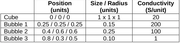
We implemented our algorithm using the commercial ‘MATLAB’ package and used it to reconstruct a simulated material distribution of three bubbles of differing size and material contained in a cube with background conductivity of 20 S/unit length. The positions, size and conductivities of the objects are as follows:

Position (units)

Size / Radius (units)

Conductivity (S/unit)

Cube 0 / 0 / 0 1 x 1 x 1 20

Bubble 1 0.25 / 0.25 / 0.25 0.15 200

Bubble 2 0.4 / 0.6 / 0.6 0.25 100

Bubble 3 0.8 / 0.3 / 0.5 0.10 1

Table 1: Positions, size and material of simulated objects

Figure 3a shows the simulated configuration, the dark areas in figure 3b indicate the electrode positions on the cube’s surface. For the simulation, we assumed a set-up of 24 electrodes on the cubes surface, four on each face, and used 24 out of the possible 276 current patterns with cross-sectional current injection to obtain better sensitivity. The contact impedance used in the complete electrode model computation was assumed 100 S/unit length. A Tikhonov regularization parameter λ=0.7x10-4was employed together with a zeroth order regularization matrix. The mesh for the recon-struction consisted of 1286 elements and 377 nodes, which corresponds to a spatial resolution of approximately 10%. After error estimator based refinement with a refinement parameter of 40% of the maximal occurring error, the node and element density increases particularly in regions of high current density. A final material-gradient refinement enhances the spatial resolution at material boundaries.

The algorithm needed eight iteration steps to converge to the material distribution given in figure 3. 2D algorithms usually require only four iteration steps to reach a final solution. This increase for three-dimensional problems is probably due to the increased ill-conditioning caused by the much larger number of degrees of freedom in the process. This could be avoided in 2D by grouping elements together and using mesh conforming refinement for the forward solution, but poses a challenge for general 3D problems.

1

2

3

1

2

3

a)

b)

Figure 3: (a) Simulated conductivity distribution, sphere parameters are given in table 1, (b) size and position of attached electrodes used for current injection and voltage measurement.

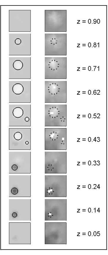
Figure 4: 2D slices through the cube at height z. Left: original conductivity distribution with indication of the spheres’ boundaries, right: reconstructed conductivity

distribution; the gaps represent interpolation errors.

employing LU decomposition for the solution on a mesh comprised of 6535 elements and 1472 nodes. All quantities were obtained using MATLAB Version 6.0 on a 500MHz AMD Athlon processor.

Mesh: 1286 elements, 377 nodes speed-up factor memory saving factor

Sparse matrix techniques 5.13 / iteration 61.2

Adaptive meshing ~3.8 ~1.27

Pure CG solver / regularised LU solver 2.36 1.02

Tikhonov Regularization / pure CG solver ~2.1

-Parallelization (8 cluster nodes) estimated 8

-Table 2: Performance improvement of tomographic reconstruction algorithms by application of optimisation techniques.

5 CONCLUSIONS AND FURTHER WORK

We have developed an efficient 3D non-linear Electrical Tomography reconstruction algorithm incorporating a regularized conjugate gradient solver and an auto-adaptive mesh refinement process. The image smoothness constraint allows for increased accuracy based on physical properties of the solution, and material-gradient dependent adaptive mesh refinement allows for better image resolution.

We show that the reconstruction performance is improved by regularizing the ill-conditioned inverse problem and other optimisations such as sparse matrix techniques and (auto-)adaptive meshing. Finally, parallel computing methods are highly applicable.

Our results indicate that it is possible to reduce the image reconstruction time towards real time by a large factor compared with ‘standard’ 3D algorithms. This increases the feasibility of performing fully nonlinear reconstructions for complex large-scale industrial and biomedical problems using standard PC technology. Future work will focus on parallelizing this algorithm for the execution on a PC cluster.

6 REFERENCES

Blott BH, Cox SJ, Daniell GJ, Caton MJ, and Nicole DA (2000). High fidelity imaging and high performance computing in nonlinear EIT.Physiol. Meas. 21(1), pp.7-14.

Blott BH, Daniell GJ and Meeson S (1998). Nonlinear reconstruction constrained by image properties in EIT.Phys. Med. Biol. 43, pp.1215–24.

Blue RS, Isaacson D, Newell JC, (2000), Real-time three-dimensional electrical impedance imaging, Physiol. Meas. 21, pp.15-26

Burnett DS, (1987),Finite element analysis, from concepts to applications, Addison-Wesley.

Cheney M, Isaacson D, Newell JC, Simske S and Goble J, (1990), NOSER: An Algorithm for Solving the Inverse Conductivity Problem,Int J Imaging Systems and Technology, Vol. 2, pp. 66-75

Committee on the Mathematics and Physics of Emerging Dynamic, (1996),Mathematics and Physics of Emerging Biomedical Imaging, Biomedical Imaging, National Research Council, USA, Online Book at http://www.nap.edu/catalog/5066.html

Groetsch CW, (1993),Inverse Problems in the Mathematical Sciences, Vieweg-Verlag, Germany

Hake, JF, (1992), Parallel Algorithms for Matrix Operations and their Performance on Multiprocessor Systems, In: Kronsjö L and Shumsherruddin D (eds.), Advances in Parallel Algorithms, Blackwell Scientific Publications, London, pp. 396-437.

Lamm P K, (1993), Inverse problems and ill-possedness, "Inverse Problems in Engineering: Theory and Practice", pp. 1-10

Molinari M, Cox SJ, Blott BH and Daniell GJ, (2001a), Adaptive Mesh Refinement Techniques for Electrical Impedance Tomography.Physiol. Meas. 22(1), pp. 91-96

Molinari M, Cox SJ, Blott BH and Daniell GJ, (2001b), Efficient non-linear electrical tomography recon-struction, submitted for publication toMeas. Sci. Technol., Special Feature on Electrical Tomography

Ollikainen J, Vauhkonen M, Kaipio JP and Karjalainen PA, (1996), Using EIT resistivity estimates in EEG inverse problems, 1st International Conference on Bioelectromagnetism, Tampere, Finland, June 9-13, 1996.

Piccolomini A L, Zama F, (1999), The conjugate gradient regularization method in Computed Tomography problems,Appl. Math. and Comp. 102, pp. 87-99

Shephard MS 1985. Automatic and Adaptive Mesh Generation. IEEE Trans. Magnetics MAG-21, pp. 2484-89.

Shewchuk J R, (1994), "An Introduction to the Conjugate Gradient Method Without the Agonizing Pain", Carnegie Mellon University, Pittsburgh, USA

Somersalo E, Cheney M and Isaacson D, (1992), Existence and uniqueness for electrode models for electric-current computed-tomography,SIAM J. Appl. Math. 52, pp. 1023-1040

Szymanski JE and Tsourlos P, (1993), The resistive tomography technique for archaeology: an introduction and review, in:Achaeologia Polona 31, pp. 5-32

Vauhkonen PJ, Vauhkonen M, Savolainen T, Kaipio JP, (1999), Three-Dimensional Electrical Impedance Tomography Based on the Complete Electrode Model, IEEE Trans. Biomed. Eng. 46(9), pp. 1150-1160

Wexler A, (1988), Electrical impedance imaging in two and three dimensions,Clin Phys Physiol Meas 9(4) Suppl A pp. 29-33

Yorkey TJ, Webster JG and Tompkins WJ, (1987), Comparing Reconstruction Algorithms for Electrical Impedance Tomography,IEEE Trans. on Biomed. Eng., BME-34, No. 11, pp. 843-852