Two Sample Tests for High Dimensional Means with Thresholding and Data Transformation

Munich Personal RePEc Archive

Two-Sample Tests for High Dimensional

Means with Thresholding and Data

Transformation

Chen, Song Xi and Li, Jun and Zhong, Pingshou

Peking University, Kent State Univeristy, Michgan State University

2014

Two-Sample Tests for High Dimensional Means

with Thresholding and Data Transformation

∗

Song Xi Chen, Jun Li and Ping-Shou Zhong

Peking University and Iowa State University, Kent State University,

and Michigan State University

Abstract

We consider testing for two-sample means of high dimensional populations by thresh-olding. Two tests are investigated, which are designed for better power performance when the two population mean vectors differ only in sparsely populated coordinates. The first test is constructed by carrying out thresholding to remove the non-signal bearing dimensions. The second test combines data transformation via the preci-sion matrix with the thresholding. The benefits of the thresholding and the data transformations are showed by a reduced variance of the test thresholding statistics, the improved power and a wider detection region of the tests. Simulation experi-ments and an empirical study are performed to confirm the theoretical findings and to demonstrate the practical implementations.

Keywords: Data Transformation; Large deviation; Large psmall n; Sparse signals;

Thresholding.

1. INTRODUCTION

Modern statistical data in biological and financial studies are increasingly high di-mensional, but with relatively small sample sizes. This is the so-called “largep, small

n” phenomenon. If the dimension p increases as the sample size n increases, many classical approaches originally designed for fixed dimension problems (Hotelling’s test and the likelihood ratio tests for the covariances) may no longer be feasible. New methods are needed for the “largep, small n” setting.

An important high dimensional inferential task is to test the equality of the mean vectors between two populations, which represent two treatments. Let Xi1· · · ,Xini

be an independent and identically distributed sample drawn from a p-dimensional distributionFi, fori= 1 and 2 respectively. The dimensionalitypcan be much larger

than the two sample sizes n1 and n2 so that p/ni → ∞. Let µi and Σi be the means

and the covariance of Fi. The primary interest is testing

H0 :µ1 =µ2 versus H1 :µ1 6=µ2. (1.1)

Hotelling’s T2 _{test has been the classical test for the above hypotheses for fixed}

dimension p and is still applicable if p _≤ n1 +n2 −2. However, as shown in Bai

and Saranadasa (1996), Hotelling’s test suffers from a significant power loss when

p/(n1+n2−2) approaches to 1 from below. When p > n1+n2−2, the test is not

applicable as the pooled sample covariance matrix, say Sn, is no longer invertible. There are proposals which modify Hotelling’s T2 _{statistic for high dimensional}

situations. Bai and Saranadasa (1996) proposed the following alteration

Mn= ( ¯X1−X¯2)T( ¯X1−X¯2)−tr(Sn)/n, (1.2)

combi-nation of U-statistics

Tn=

1

n1(n1 −1)

n1

X

i6=j

X₁T_iX1j+

1

n2(n2 −1)

n2

X

i6=j

X₂T_iX2j −

2

n1n2

n1

X

i n2

X

j

X₁T_iX2j,(1.3)

and showed that the corresponding test can operate under much relaxed regimes regarding the dimensionality and sample size constraint and without assuming Σ1 =

Σ2. Srivastava, Katayama and Kano (2013) proposed using the diagonal matrix of

the sample variance matrice to replaceSn under the normality. These three tests are

basically all targeted on a weighted L2 norms betweenµ1 and µ2. In a development

in another direction, Cai, Liu and Xia (2014) proposed a test based on the max-norm of marginal t-statistics. More importantly, they implemented a data transformation which is designed to increase the signal strength under sparsity as discovered early in Hall and Jin (2010) in their innovated higher criticism test for the one sample problem.

The L2 norm based tests are known to be effective in detecting dense signals in

the sense that the differences between µ1 and µ2 are populated over a large number

of the precision matrix via the Cholesky decomposition with the banding approach (Bickel and Levina, 2008a, 2008b). It is shown that the test with the thresholding and the data transformation has a lower detection boundary than that without the data transformation, and can be lower than the detection boundary of an Oracle test without data transformation.

The rest of the paper is organized as follows. We analyze the thresholding test and its relative power performance to the CQ test and the Oracle test in Section 2. A multi-level thresholding test is proposed in Section 3 for detecting faint signals. Section 4 considers a data transformation with an estimated precision matrix. Sim-ulation results are presented in Section 5. Section 6 reports an empirical study to select differentially expressed gene-sets for a human breast cancer data set. Section 7 concludes the paper with discussions. All technical details are relegated to the Appendix.

2. THRESHOLDING TEST

We first outline the CQ statistic before introducing the thresholding approach. The statistic (1.3) can be written as Tn=Ppk=1Tnk where

Tnk =

1

n1(n1−1)

n1

X

i6=j

X₁(k_i)X₁(k_j)+ 1

n2(n2−1)

n2

X

i6=j

X₂(k_i)X₂(k_j)

− _n2

1n2

n1

X

i n2

X

j

X₁(k_i)X₂(k_j), (2.1)

and X_ij(k) represents the k-th component of Xij. It can be readily shown that Tnk is

unbiased to (µ1k−µ2k)2, which may be viewed as the amount of signal in the k-th

dimension.

To facilitate simpler notations, we modify the test statistic Tn by standardizing

eachTnk byσ1,kk/n1+σ2,kk/n2, the variance of ¯X1(k)−X¯ (k)

2 , if bothσ1,kk andσ2,kk are

ˆ

σ2,kk are the usual sample variance estimates at the k-th dimension. This will make

the CQ test invariant under the scale transformation; see Feng, Zou, Wang and Zhu (2013) for a related investigation. To expedite our discussion, we assume σ2

i,kk are

known and equal to one without loss of generality. This leads to a modified version of the CQ statistic

˜

Tn=n p

X

k=1

Tnk, (2.2)

wheren =n1n2/(n1+n2). Under the same setting, a modified version of the Bai and

Saranadasa (BS) test statistic is

˜

Mn =n p

X

k=1

Mnk−p, (2.3)

where Mnk = ( ¯X1(k)−X¯ (k) 2 )2.

Let δk = µ1k−µ2k and Sβ = {k : δk 6= 0} be the set of locations of the signals

δk such that |Sβ| = p1−β where β ∈ (0,1) is the sparsity parameter. Basically, the

sparsity of the signal increases asβis closer to 1. Under the sparsity, an overwhelming number of Tnk carry no signals. However, including them increases the variance of

the test statistic, and dilutes the signal to noise ratio of the test; and thus hampers the power of the test.

Let us now analyze the standardized CQ test under the sparsity. Define

ρkl = Cov

√

n( ¯X₁(k)₋X¯₂(k)),√n( ¯X₁(l)₋X¯₂(l))

=n(σ1,kl/n1+σ2,kl/n2). (2.4)

Similar to the derivation in Chen and Qin (2010), the variance of ˜Tn under H0 is

σ_Tn,2˜ ₀ = 2p+ 2

X

i6=j

ρ2_ij,

and that under H1 is

σ_Tn,2˜ ₁ = 2p+ 2

X

i6=j

ρ2_ij + 4n X

k,l∈Sβ

It can be seen that σ2 ˜

Tn,1 ≥ σ 2

˜

Tn,0 since the last term of σ 2

˜

Tn,1 is nonnegative due to

R= (ρij)p×p being non-negative definite.

Under a general multivariate model and some conditions on the covariance matri-ces, the asymptotic normality of ˜Tn can be established (Chen and Qin, 2010):

˜

Tn− ||µ1−µ2||2

σ_Tn,˜ ₁

d

−

→N(0,1), asp_{→ ∞}andn _{→ ∞}.

This implies the modified CQ test that rejects H0 if ˜Tn/σˆ_Tn,˜ ₀ > zα where zα is the

upper α quantile of N(0,1) and ˆσ_Tn,˜ ₀ is a consistent estimator of σ_Tn,˜ ₀.

Let ¯δ2 ₌ P

k∈Sβ n δ2k/p1−β represent the average standardized signal. The power

of the test is

β_Tn˜ (||µ1−µ2||) = Φ

− σ_σTn,˜ 0 ˜

Tn,1

zα+

p1−β_δ¯2

σ_Tn,˜ ₁

,

where Φ(_·) is the distribution function of N(0,1). Since σ2 ˜

Tn,1 ≥ σ 2

˜

Tn,0, the first term

within Φ(_·) is bounded. Then, the power of the test is largely determined by the second term

SNR_Tn˜ =: p 1−β_¯δ2

q

2p+ 2P_i6=jρ2

ij + 4n

P

k,l∈Sβδkδlρkl

, (2.6)

which is called the signal to noise ratio of the test since the numerator is the average signal strength and the denominator is the standard deviation of the test statistic under H1. An inspection reveals that while the numerator of SNR_Tn˜ is contributed

only by those signal bearing dimensions, the standard deviation in the denominator is contributed by all Tnk including those with non-signals.

Specifically, if Σ1 =Σ2 =Ip,

SNR_Tn˜ =

p1−β_δ¯2

p

2p+ 4p1−β_δ¯2.

Hence, if the sparsity β >1/2 and the average signal ¯δ=o(pβ/2−1/4_{), SNR} ˜

Tn =o(1).

loss is that the variance of ˜Tn is much inflated by including those non-signal bearing

Tnk.

To put the above analysis in prospective, we consider an Oracle test which has the knowledge of the possible signal bearing set Sβ (with slight abuse of notation),

which is much smaller than the entire set of dimensions. The Oracle is only a semi-Oracle as he does not know the exact dimensions of the signals other than that they are within Sβ.

The Oracle test statistic is

On=n

X

k∈Sβ

Tnk, . (2.7)

Similar to the derivation of (2.5), the variance ofOn under H0 is

σ2_On,0 = 2p1−β+ 2 X

i6=j∈Sβ

ρ2_ij,

and that under H1 is

σ_On,2 ₁ = 2p1−β + 2 X

i6=j∈Sβ

ρ2_ij + 4n X

k,l∈Sβ

δkδlρkl. (2.8)

Comparingσ2

On,1 withσ_Tn,2˜ ₁ in (2.5), we see that the first term ofσ2On,1 is much smaller

than that of σ2 ˜

Tn,1. It may be shown that under the same conditions that establish

the asymptotic normality of ˜Tn,

On− ||µ1−µ2||2

σOn,1

d

−

→N(0,1), asp_{→ ∞}and n_{→ ∞},

which leads to the Oracle test that rejects H0 if On/ˆσOn,0 > zα where ˆσOn,0 is a ratio

consistent estimator of σOn,0.

The asymptotic normality implies that the power of the Oracle test is

βOn(||µ1−µ2||) = Φ

− σ_σOn,0

On,1

zα+

p1−β_δ¯2

σOn,1

It is largely determined by

SNROn =:

p1−β_δ¯2

q

2p1−β_{+ 2}P

i6=j∈Sβρ2ij + 4n

P

k,l∈Sβδkδlρkl

, (2.9)

which is much larger than SNR_Tn˜ since σOn,2 1 ≪σ_Tn,2˜ ₁. If Σ1 =Σ2 =Ip,

SNROn =

p1−β_δ¯2

p

2p1−β_{+ 4p}1−β_δ¯2 =

p1−2βδ¯2

√

2 + 4¯δ2, (2.10)

that tends to infinity for β > 1/2 as long as ¯δ is a large order of pβ/4−1/4_{, which is}

much smaller thanpβ/2−1/4 _{for the CQ test, indicating the test is able to detect much}

fainter signal.

The reason that the Oracle test has better power is that all the excluded sions are definitely non-signal bearing and those included have much smaller dimen-sions. In reality, the locations of those non-signal bearing dimensions are unknown. However, thresholding can be carried out to exclude those non-signal bearing dimen-sions. Based on the large deviation results (Petrov, 1995), we use a thresholding level

λn(s) = 2slogpfors ∈(0,1) to strike a balance between removing non-signal bearing

Tnk while maintaining those with signals. The thresholding test statistic is

L1(s) =

p

X

k=1

n TnkI

n Tnk + 1> λn(s)

, (2.11)

where I(_·) is the indicator function.

We can also carry out the thresholding on BS test statistic (2.3), which leads to

L2(s) =

p

X

k=1

n( ¯X1(k)−X¯ (k) 2 )2−1

I

n( ¯X1(k)−X¯ (k)

2 )2 > λn(s)

. (2.12)

As we will show later, both L1(s) and L2(s) have very similar properties. Therefore,

we choose Ln(s) to refer to either L1(s) or L2(s).

notion ofα-mixing to quantify the dependence among the components of the random vector X = (X(1)_{,· · · , X}(p)₎T_.

For any integers a < b, define _FX,(a,b) to be the σ-algebra generated by {X(m) :

m_∈(a, b)_} and define the α-mixing coefficient

αX(k) = sup

m∈N,A∈FX,(1,m),B∈FX,(m+k,∞)

|P(A_∩B)₋P(A)P(B)_|.

The following conditions are assumed in our analysis.

(C1): Asn _{→ ∞},p_{→ ∞} and logp=o(n1/3_).

(C2): Let Xij = µi +Wij. There exists a positive constant H such that for

h_∈[₋H, H]2_{, E{e}hT_·[(W(k)

ij )2,(W

(l)

ij )2]}<∞ for k6=l.

(C3): The sequence of random variables_{X_ij(l)_}lp₌₁ isα-mixing such thatαX(k)≤

Cαk _{for some α ∈ (0,1) and a positive constant C, and ρ}

kl defined in (2.4) are

summable such that Pp_l=1|ρkl|<∞ for any k∈ {1,· · · , p}.

Condition (C1) specifies the growth rate of dimension prelative tonunder which the large deviation results can be applied to derive the means and variances of the test statistics. Condition (C2) assumes that (X_ij(k), X_ij(l)) has a bivariate sub-Gaussian distribution, which is more general than the Gaussian distribution. Condition (C3) prescribes weak dependence among the column components of the random vector, which is commonly assumed in time series analysis.

Derivations given in Appendix leading to (A.1) and (A.2) show that the mean of the thresholding test statistic Ln(s) is

µLn(s) =

2

√

2π(2slogp)

1

2p1−s+ X

k∈Sβ

{n δ_k2I(n δ_k2 >2slogp)

+(2slogp) ¯Φ(η_k−)I(n δ_k2 <2slogp)_}

and the variance is

σ2_Ln(s) =

2

√

2π{(2slogp)

3

2 + (2slogp)12}p1−s+ X

k,l∈Sβ

(4nδkδlρkl+ 2ρ2kl)

× I(nδ_k2 >2slogp)I(n δ_l2 >2slogp) + X

k∈Sβ

(2slogp)2Φ(¯ η_k−)

× I(n δ_k2 <2slogp)

{1 +o(1)_}, (2.14)

where ¯Φ = 1₋Φ andη_k−= (2slogp)1/2_−n1/2_δ

k.

Theorem 1. Assume Conditions (C1)-(C3). For any s_∈(0,1),

σ−_Ln1_(s)Ln(s)−µLn(s)

d

−

→N(0,1).

LetµLn(s),0 andσLn(s),0 be the mean and variance underH0 which can be obtained

by ignoring the summation terms in (2.13) and (2.14). Then, Theorem 1 implies an asymptotic α level test that rejects H0 if

Ln(s)> zασˆLn(s),0+ ˆµLn(s),0, (2.15)

where ˆµLn(s),0 and ˆσLn(s),0 are consistent estimators of µLn(s),0 and σLn(s),0 satisfying

µLn(s),0−µˆLn(s),0 =o{σLn(s),0} and σˆLn(s),0/σLn(s),0

p

→1. (2.16)

If all the signals δ2

k are strong such that n δ2k >2logp, choosing s = 1− such that

(1₋s) log(p) =o(1) leads to

µLn(s) =

2

√

2π(2logp)

1 2 +

X

k∈Sβ

n δ_k2

{1 +o(1)_},

and

σ2_Ln(s) =

2

√

2π{(2logp)

3

2 + (2logp) 1 2}+

X

k,l∈Sβ

(4n δkδlρkl+ 2ρ2kl)

{1 +o(1)_}.

Except for a slowly varying logarithm function ofp,σ2

Ln(s) has the same leading order

variance of the Oracle statistic

σ2_On,1 = X

k,l∈Sβ

4n δkδlρkl+ 2ρ2kl

indicating the effectiveness of the thresholding under the strong signal situation. With the same choice of s for strong signals case, µLn(s),0 and σ_Ln2 _(s),0 can be respectively

estimated by

ˆ

µLn,0 =

2

√

2π(2logp)

1

2 and σˆ2

Ln,0 =

2

√

2π{(2logp)

3

2 + (2logp) 1 2}.

It can be shown that (2.16) is satisfied under (C1) and thus can be employed in the formulation of a test procedure.

The asymptotic power of the thresholding test (2.15) is

βLn(||µ1−µ2||) = Φ

−zα_σσLn(s),0

Ln(s),1

+µLn(s),1−µLn(s),0

σLn(s),1

,

which, similar to the CQ and the Oracle tests, is largely determined by

SNRLn =:

µLn(s),1−µLn(s),0

σLn(s),1

= p

1−β_δ¯2

q

2Lp+ 2p1−β+ 2P_k6=l∈Sβρ2kl+ 4n

P

k,l∈Sβδkδlρkl

, (2.17)

which is much larger than that of the CQ test in (2.6) and differs from that of the Oracle test given in (2.9) only by a slowly varying multi-logp function Lp. This

echoes that established in Fan (1996) for Gaussian data with no dependence among the column components of the data.

3. MULTI-LEVEL THRESHOLDING

It is shown in Section 2 that if all the signals are strong such thatnδk>2logp, a single

thresholding with s = 1− _{improves significantly the power of the test and attains}

nearly the power of the Oracle test. However, if some signals are weak such that

n δ2

k = 2rlogp with r <1 for some k ∈ Sβ, the thresholding has to be administrated

higher criticism test (Donoho and Jin, 2004) which effectively combines many levels of thresholding together to formulate a higher criticism (HC) criterion. Zhong, Chen and Xu (2013) proposed a more powerful test procedure than the HC test under sparsity and data dependence. Both Donoho and Jin (2004)’s HC test and the test proposed in Zhong et al. (2013) are for one sample, and both did not provide much details on the power performance.

The multi-level thresholding statistic is

MLn = max s∈(0,1−η)

Ln(s)−µˆLn(s),0

ˆ

σLn(s),0

. (3.1)

Maximizing over the thresholding statistics at multiple levels allows faint and un-known signals to be captured. Since both ˆµLn(s),0 and ˆσLn(s),0 are monotonically

decreasing and Ln(s) contains indicator functions, provided (2.16) is satisfied, it

can be shown that the maximization in (3.1) is attained over _Sn = {sk : sk =

n( ¯X1(k)−X¯ (k)

1 )2/(2logp),fork= 1,· · ·, p} ∩(0,1−η) so that

MLn = max s∈Sn

Ln(s)−µˆLn(s),0

ˆ

σLn(s),0

. (3.2)

The following theorem shows that MLn is asymptotically Gumbel distributed.

Theorem 2. Assume Conditions (C1)-(C3) and condition (2.16) is satisfied. Then under H0,

P

a(logp)MLn −b(logp, η)≤x

→exp(₋e−x),

where functionsa(y) = (2logy)12 and b(y, η) = 2logy+ 2−1loglogy−2−1log{ 4π

(1−η)2}.

The theorem implies that a two-sample multi-level thresholding test of asymptotic

α level rejects H0 if

MLn ≥Gα ={qα+b(logp, η)}/a(logp), (3.3)

Define

̺(β) =

    

β₋ 1₂, 1_{2 ≤}β_≤ 3₄; (1₋√1₋β)2_, 3

4 < β <1.

(3.4)

Ingster (1997) shows thatr=̺(β) is the optimal detection boundary for uncorrelated Gaussian data in the sense that when (r, β) lays above the phase diagram r= ̺(β), there are tests whose probabilities of type I and type II errors converge to zero simul-taneously as n _{→ ∞}, and if (r, β) is below the phase diagram, no such test exists. Donoho and Jin (2004) showed that the HC test attains r = ̺(β) as the detection boundary when Xi are IID N(µ, Ip) data. Zhong et al. (2013) showed that the L1

and L2-versions of the HC tests also attain r = ̺(β) as the detection boundary for

non-Gaussian data with column-wise dependence, and have more attractive power for (r, β) further above the detection boundary.

Theorem 3. Assume Conditions (C1)-(C3) and ˆµLn(s),0 and ˆσLn(s),0 satisfy

(2.16). If r > ̺(β), the sum of type I and II errors of the multi-level thresholding test converges to zero when α = ¯Φ_{(logp)ǫ_{} →} 0 for an arbitrarily small ǫ > 0 as

n _{→ ∞}. If r < ̺(β), the sum of type I and II errors of the multi-level thresholding test converges to 1 as α_→0 andn _{→ ∞}.

Theorem 3 implies that the two-sample multi-level thresholding test also attains

r = ̺(β) as the detection boundary in the current two-sample test setting of non-parametric distributional assumption. This means that the test can asymptotically distinguishH1 fromH0 for any (r, β) above the detection boundary. If the mean and

variance estimators ˆµLn(s),0 and ˆσLn(s),0 do not satisfy (2.16), the detection boundary

4. TEST WITH DATA TRANSFORMATION

We consider in this section another way for power improvement, which involves en-hancing the signal strength by data rotation, inspired by the works of Hall and Jin (2010) and Cai, Liu and Xia (2014). We will show in this section that the signal en-hancement can be achieved by transforming the data via an estimate of the inverse of a mixture ofΣ1 and Σ2. Transforming data to achieve better power has been consid-ered in Hall and Jin (2010) in their innovated higher criticism test under dependence and Cai, Liu and Xia (2014) in their max-norm based test. The transformation used in Hall and Jin (2010) was via a banded Cholesky factor, and that adopted in Cai, Liu and Xia (2014) was via the CLIME estimator of the inverse of the covariance matrix (the precision matrix) proposed in Cai, Liu and Luo (2011).

Consider a bandable covariance matrix class

V(ǫ0, C, α) =

Σ: 0< ǫ0 ≤λ_min(Σ)≤λmax(Σ)≤ǫ−01, α >0, |σij| ≤C(1 +|i−j|)−(α+1) for all i, j :|i−j| ≥1

.

This class of matrices satisfies both the banding and thresholding conditions of Bickel and Levina (2008b). Hall and Jin (2010) also considered this class when they proposed the innovated higher criticism test under dependence.

(C4): Both Σ1 and Σ2 belong to the matrix class V(ǫ0, C, α).

Although both (C3) and (C4) assume the weak dependence among the column components of the random vector Xij, imposing (C4) ensures that the banding

esti-mation of the covarianvce matrix which makes the transformed data are still weakly dependent. To appreciate this, let Ω = _{(1₋κ)Σ1 +κΣ2_}−1 _{= (ω}

ij)p×p. We first

assume Ω is known to gain insight on the test. Rather than transforming the data via Ω, we transform it via

Ω(τ) =

ωijI(|i−j| ≤τ)

p×p

a banded version of Ω for an integer τ between 1 and p₋1. There are two reasons to use Ω(τ). One is that the signal enhancement is facilitated mainly by elements of

Ω close to the main diagonal. Another is that the banding maintains the α-mixing structure of the transformed data provided k₋2τ _{→ ∞}. Since both Σ1 andΣ2 have their off-diagonal entries decaying to zero at polynomial rates,Ωhas the same rate of decay as well (Jaffard, 1990; Sun, 2005; Gr¨ochenig, and Leinert, 2006), which ensures that the transformed data are still weakly dependent.

The two transformed samples are

{Z1j(τ) = Ω(τ)X1j : 1≤j ≤n1} and {Z2j(τ) = Ω(τ)X2j : 1≤j ≤n2}.

Let̟kk(τ) = Var{√n( ¯Z1(k)(τ)−Z¯ (k)

2 (τ))}be the counterpart ofn(σ1,kk/n1+σ2,kk/n2)

for the transformed data where ¯Z_i(k)(τ) = n−_i 1Pnj_j=1Z_ij(k)(τ) for i = 1,2. Lemmas 5 and 7 in Appendix show that there exists a constant C > 1 such that

̟kk(τ) =ωkk+O(τ−C) and ωkk>1. (4.1)

We have two ways to construct the transformed thresholding test statistic by replacing Xij with Zij(τ) in either (2.11) or (2.12). Alhough both have similar properties, the latter which has the form

Jn(s, τ) = p

X

k=1

n( ¯Z₁(k)(τ)₋Z¯₂(k)(τ))2

̟kk(τ) −

1

I

n( ¯Z₁(k)(τ)₋Z¯₂(k)(τ))2

̟kk(τ)

> λn(s)

(4.2)

is easier to work with, which we will present in the following.

Let δ_Ω(τ) = (δΩ(τ),1,· · · , δΩ(τ),p)T where

δ_Ω(τ),k =

X

l

Ωkl(τ)δl=

X

l∈Sβ

ωklδlI(|k−l| ≤τ) (4.3)

to (2.13) and (2.14), the mean and variance of the transformed statistic Jn(s, τ) are

µJn(s,τ) =

2

√

2π(2slogp)

1

2p1−s+ X

k∈SΩ(τ),β

{n δ

2

Ω(τ),k

̟kk(τ)

I(n δ

2

Ω(τ),k

̟kk(τ)

>2slogp)

+ (2slogp) ¯Φ(η−_Ω(τ)k)I(n δ

2

Ω(τ),k

̟kk(τ)

<2slogp)_}

{1 +o(1)_}, (4.4)

and

σJn2 (s,τ) =

2

√

2π{(2slogp)

3

2 + (2slogp) 1

2}p1−s+

X

k,l∈SΩ(τ),β

(4n δΩ(τ),k ̟_kk1/2(τ)

δ̟(τ),l

̟1_ll/2(τ)ρΩ,kl

+ 2ρ2_Ω,kl)I(n δ

2

Ω(τ),k

̟kk(τ)

>2slogp)I(n δ

2

Ω(τ),l

̟ll(τ)

>2slogp)

+ X

k∈SΩ(τ),β

(2slogp)2Φ(¯ η_Ω−_(τ)k)I(n δ

2

Ω(τ),k

̟kk(τ)

<2slogp)

{1 +o(1)_}, (4.5)

where S_Ω(τ),β ={k :δΩ(τ),k 6= 0}is the set of locations of the non-zero signals δΩ(τ),k,

η−_Ω(τ)k = (2slogp)1/2_−n1/2_δ

Ω(τ),k/̟kk(τ)1/2 and

ρ_Ω,kl = Cov

√

n( ¯Z1(k)(τ)−Z¯ (k) 2 (τ))

p

̟kk(τ)

,

√

n( ¯Z1(l)(τ)−Z¯ (l) 2 (τ))

p

̟ll(τ)

.

In practice, the precision matrix Ω is unknown and needs to be estimated. We consider the Cholesky decomposition and the banding approach similar to that in Bickel and Levina (2008a). Define Ykl = X1k − p₁₋κ_κX2l for k = 1,· · · , n1 and

l = 1,_{· · ·}, n2, where κ = lim

n→∞n1/(n1 +n2). Then Var(Ykl) = Σw ≡ Σ1 +

κ

1−κΣ2.

Thus, to estimate Ω= (1₋κ)−1_Σ−1

w , we only need to estimate Σ−w1.

LetY be an IID copy ofYklfor any fixedk andlsuch thatY = (Y(1),· · ·, Y(p))T.

For j = 1,_{· · ·} , p, define ˆY(j) _{= a}T

jW(j) where aj = {Var(W(j))}−1Cov( ˆY(j),W(j))

and W(j)_{= (Y}(1)_{,· · · , Y}(j−1)₎T_{. Let ǫ}

j =Y(j)−Yˆ(j) andd2j = Var(ǫj), andAbe the

lower triangular matrix with thej-th row being (aT

j,0p−j+1) andD= diag(d21,· · · , d2p)

where0smeans a vector of 0 with lengths. Then, the population version of Cholesky

decomposition is Σ−1

w = (I−A)TD−1(I−A).

The banded estimators forAandD(Bickel and Levina, 2008a) can be used in the case ofp >min_{n1, n2}. Specifically, letYn,kl =X1k−

q

n1

n2X2l:= (Y

(1)

n,kl,· · ·, Y

(p)

Given a τ, regress Y_n,kl(j) onY(_n,kl,j) _−τ = (Y_n,kl(j−τ),_{· · ·} , Y_n,kl(j−1))T _{to obtain the least square}

estimate of aj,τ = (aj−τ,· · ·, aj−1)T:

ˆ

aj,τ = ( n1 X k=1 n2 X l=1

Y_n,kl,(j) _−τY_n,kl,(j)T_−τ)−1

n1 X k=1 n2 X l=1

Y(_n,kl,j) _−τY_n,kl(j) .

Put ˆaT

j = (0Tτ−1,aˆTj,τ,0Tp−j+1) be the j-th row of a lower triangular matrix ˆAτ and

ˆ

Dτ = diag(d21,τ,· · ·, dp,τ2 ) where d2j,τ = n11n2

Pn1

k=1

Pn2

l=1(Y (j)

n,kl −aˆTj,τY

(j)

n,kl,−τ)2. Thus,

the estimator ofΣ−1

w is

d

Σ−1

w = (I −Aˆτ)TDˆτ−1(I−Aˆτ), (4.6)

which results in ˆΩτ ={1−n1/(n1+n2)}−1Σd−w1.

The consistency of ˆΩτ toΩbasically follows the proof of Theorem 3 in Bickel and

Levina (2008a) with a main difference that replaces the exponential tail inequality for a sample mean in Lemma A.3 of their paper to an exponential inequality of a two-sample U-statistics. Moreover, if the banding parameter τ _≍ (n−1_logp)−2(α1+1)

and n−1_{logp=o(1), it can be shown that}

||Ωˆτ −Ω||=Op

(logp/n)2(αα+1)

,

where _{k · k}is the spectral norm.

The transformed thresholding test statistic based on _{Zˆ1i = ˆΩτX1i : 1≤i≤n1}

and _{Zˆ2i = ˆΩτX2i : 1≤i≤n2} is

ˆ

Jn(s, τ) = p

X

k=1

n(Z¯ˆ₁(k)₋Z¯ˆ₂(k))2

ˆ

ωkk −

1

I

n(Z¯ˆ₁(k)₋Z¯ˆ₂(k))2

ˆ

ωkk

> λn(s)

. (4.7)

To consistently estimate Ω, we require that τ _≍ (n−1_logp)−2(α1+1). This

require-ment leads to a modification on the range of the thresholding levels as shown in the next theorem.

Theorem 4. Assume Conditions (C1)-(C4). If p = n1/θ _{for 0 < θ < 1 and}

τ _≍(n−1_logp)−2(α1+1)_{, then for any s∈(1−θ,1),}

σ_Jn−1_(s,τ),0

ˆ

Jn(s, τ)−µJn(s,τ),0

d

−

The restriction on the thresholding levelsin Theorem 4 is to ensure the estimation error of ˆΩτ is negligible. Similar restriction is provisioned in Delaigle et al. (2011) and

Zhong et al. (2013). Note that ifθ is arbitrarily close to 0, pwill grow exponentially fast with n.

A single-level thresholding test based on the transformed data rejects H0 if

ˆ

Jn(s, τ)> zασˆJn(s,τ),0 + ˆµJn(s,τ),0,

where ˆµJn(s,τ),0 and ˆσ2Jn(s,τ),0 are, respectively, consistent estimators of

µJn(s,τ),0 =

2

√

2π(2slogp)

1 2p1−s

{1 +o(1)_},

and

σ2_Jn(s,τ),0 =

2

√

2π{(2slogp)

3

2 + (2slogp)12}p1−s

{1 +o(1)_},

satisfying µJn(s,τ),0−µˆJn(s,τ),0 =o{σJn(s,τ),0} and σˆJn(s,τ),0/σJn(s,τ),0

p

→1.

From Theorem 4, the asymptotic power of the transformed thresholding test is

β_Jnˆ _(s,τ)(||µ1−µ2||) = Φ

−zασJn(s,τ),0

σJn(s,τ),1

+ µJn(s,τ),1−µJn(s,τ),0

σJn(s,τ),1

,

which is determined by

SNR_Jnˆ_(s,τ)=:

µJn(s,τ),1 −µJn(s,τ),0

σJn(s,τ),1

.

Therefore, to compare with the thresholding test without transformation, it is equiva-lent to compare SNR_Jnˆ_(s,τ)to SNRLn. To this end, we assume the following regarding

the distribution of the non-zeroδk inSβ.

(C5): The elements ofSβ are randomly distributed among {1,2,· · · , p}.

Under Conditions (C1)-(C5), Lemma 8 in the Appendix shows that with proba-bility approaching to 1,

which holds for both strong and weak signals. Hence, the transformed threshold-ing test is more powerful regardless of the underlythreshold-ing signal strength for randomly allocated signals.

Similar toMLn defined in (3.2) for weaker signals, a multi-level thresholding

statis-tic for transformed data is

M_Jnˆ = max

s∈Tn

ˆ

Jn(s, τ)−µˆJn(s,τ),0

ˆ

σJn(s,τ),0

, (4.9)

where Tn ={sk :sk =n(Z¯ˆ1(k)−Z¯ˆ (k)

2 )2/(2logpωˆkk) for k = 1,· · · , p} ∩(1−θ,1−η⋆)

for arbitrarily small η⋆_{. The asymptotic distribution of M}

ˆ

Jn is given in the following

Theorem.

Theorem 5. Assume Conditions (C1)-(C4), p = n1/θ _{for 0 < θ < 1 and}

τ _≍(n−1_logp)−2(α1+1). Then under H

0,

P

a(logp)M_Jnˆ −b(logp, θ−η⋆)≤x

→exp(₋e−x),

where functionsa(_·) and b(_·,_·) are defined in Theorem 2.

The theorem implies an asymptotically α level test that rejectsH0 if

M_Jnˆ ≥ {qα+b(logp, θ−η⋆)}/a(logp). (4.10)

parametric bootstrap approximation to the null distribution of the multi-level thresh-olding statistics with and without the data transformation. We first estimate Σi by

ˆ

Σi for i= 1,2 through the Cholesky decomposition which can be obtained by

invert-ing the one-sample version of (4.6) based on the samples _{X1j}jn=11 and {X2j}nj=12 ,

respectively. Bootstrap resamples are generated repeatedly from N(0,Σˆi) which

al-lows us to obtain the bootstrap copies of the statistic MLn defined in (3.2), namely

M_Ln∗,(1)(s),_{· · ·}, M_Ln∗,(B)(s), afterB repetitions. We use_{M_Ln∗,(b)_}B

b=1 to obtain the

empir-ical null distribution of the multi-level thresholding statistic. The same parametric bootstrapping method can be also applied to the transformed multi-level thresholding statistic.

We have shown that the transformed thresholding test has a better power perfor-mance than the thresholding test without the transformation. We are to show that the transformed multi-level thresholding test has lower detection boundary than the multi-level thresholding test without transformation.

To define the detection boundary of the transformed multi-level thresholding test, let

ω = lim_p→∞

min

1≤k≤pωkk

and ω¯ = limp→∞

max

1≤k≤pωkk

.

Results in (4.1) imply that ω and ¯ω _≥1. Define

̺θ(β) =

          

(√1₋θ₋q1₋β₋ θ

2)

2_, 1

2 ≤β ≤

3−θ

4 ;

β₋ 1₂, 3−₄θ _≤β _≤ 3₄; (1₋√1₋β)2_, 3

4 < β <1.

(4.11)

Theorem 6. Assume Conditions (C1)-(C5).

(a) When Ω is known, if r < ω¯−1 _{·̺(β), the sum of type I and II errors of the}

thresholding test converges to zero whenα= ¯Φ_{(logp)ǫ_{} →0 for an arbitrarily}

small ǫ >0 as n_{→ ∞}.

(b) When Ω is unknown and p = n1/θ _{for 0 < θ < 1, then if r < ω¯}−1 _·̺

θ(β),

the sum of type I and II errors of the transformed multi-level thresholding test converges to 1 asα_→0 andn _{→ ∞}; ifr > ω−1_·̺

θ(β), the sum of type I and II

errors of the transformed multi-level thresholding test converges to zero when

α= ¯Φ_{(logp)ǫ_{} →0 for an arbitrarily small ǫ >0 as n → ∞.}

Hall and Jin (2010) has shown that utilizing the dependence can lower the de-tection boundary r = ̺(β) for Gaussian data with known covariance matrix. We demonstrate in Theorem 6 that the detection boundary can be lowered respectively for the transformed multi-level thresholding test withΩbeing known or unknown for sub-Gaussian data with estimated precision matrix. The theorem shows that there is a cost associated with using the estimated precision matrix in terms of a higher detetction boundary and more restriction on the pand n relationship.

5. SIMULATION STUDY

In this section, the simulation was designed to confirm the performance of the two multi-level thresholding tests defined in (3.2) and (4.9) without and with transfor-mation. We also experimented the test of Chen and Qin (2010) given in (1.3), the Oracle test in (2.7), and two tests proposed by Cai, Liu and Xia (2014). The latter tests are based on the max-norm statistics

G(I) = max

1≤k≤pn( ¯X

(k)

1 −X¯

(k)

2 )2 and G( ˆΩ) = max 1≤k≤p

n(Z¯ˆ₁(k)₋Z¯ˆ₂(k))2

ˆ

ωkk

,

without and with transformation, where ˆωkkwere estimates of the diagonal elements of

Ω. Cai, Liu and Xia (2014) showed thatG(I) andG( ˆΩ) converge to the type I extreme value distribution with cumulative distribution function exp(₋√1

was used to formulate the test procedures based on the two max-norm statistics. Cai, Liu and Xia (2014) employed the CLIME estimator based on a constrained l1

minimization estimator of Cai, Liu and Luo (2011) to estimate Ω. Since we use the Cholesky decomposition with banding to estimateΩin the transformed thresholding test, we used the estimated ˆωkkfrom the approach in the formulation of the max-norm

statistics.

In the simulation experiments, the two random samples _{X1j}nj=11 and {X2j}nj=12

were generated according to the following multivariate model

Xij =Σ1i/2Zij +µi,

where the innovations Zij are IID p-dimensional random vectors with independent components such that E(Zij) = 0 and Var(Zij) = Ip. We considered two types

of innovations: the Gaussian where Zij _∼ N(0, Ip) and the Gamma where each

component ofZij is standardized Gamma(4,0.5) such that it has zero mean and unit

variance. For simplicity, we assigned µ1 = µ2 = 0 under H0; and under H1, µ1 = 0

and µ2 had [p1−β] non-zero entries of equal value, which were uniformly allocated

among _{1,_{· · ·} , p_}. Here [a] denotes the integer part of a. The values of the nonzero entries were p2rlogp/n for a set of r-values ranging evenly from 0.1 to 0.4. The covariance matrices Σ1 = Σ2 =: Σ = (σij) where σij = ρ|i−j| for 1 ≤ i, j ≤ p and

ρ= 0.6. The dimensionpwas 200 and 600, respectively and the sample sizesn1 = 30

and n2 = 40.

The banding width parameter τ in the estimation of Ω was chosen according to the data-driven procedure proposed by Bickel and Levina (2008a), which is described as follows. For a given data set, we divided it into two subsamples by repeated (N times) random data split. For the l-th split, l _{∈ {}1,_{· · ·} , N_}, we let ˆΣ(τl) =

{(I₋Aˆτ(l))′}−1Dˆτ(l)(I−Aˆ(τl))−1 be the Cholesky decomposition of Σobtained from the

and ˆD(τl). Also we letSn(l) be the sample covariance matrix obtained from the second

subsample. Then the banding parameter τ is selected as

ˆ

τ = min

τ

1

N

N

X

l=1

||Σˆ(_τl)₋S_n(l)_||F, (5.1)

where _{|| · ||}F denotes the Frobenius norm.

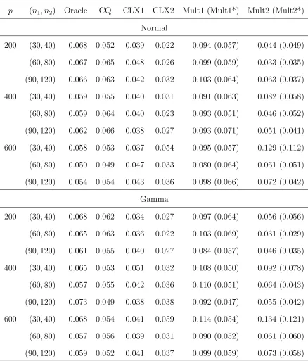
Table 1 reports the empirical sizes of the multi-thresholding tests with the data transformation (Mult2) and without the data transformation (Mult1), and Cai, Liu and Xia’s max-norm tests with (CLX2) and without (CLX1) the data transforma-tion. It also provides the empirical sizes for Mult1 and Mult2 with the bootstrap approximation of the critical values as described in Section 4. We observe that the empirical sizes of the two threshodling tests tended to be larger than the nominal 5% level due to a slow convergence to the extreme value distribution. The proposed parametric bootstrap calibration can significantly improve the size.

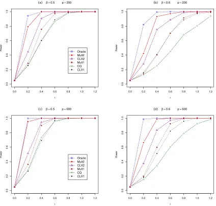
To make the power comparison fair, we pre-adjusted the nominal significant levels of all tests such that their empirical sizes were all close to 0.05. We obtain the average empirical power curves (called power profiles) plotted with respect to r and

β under each of the simulation settings outlined above based on 1000 simulations. We observed only some very small change in the power profiles when the underlying distribution was switched from the Gaussian to the Gamma, which confirmed the nonparametric nature of the tests considered. Due to the space limitation, we only display in the following the power profiles based on the Gaussian data, and those for the Gamma innovations are given in the supplementary material.

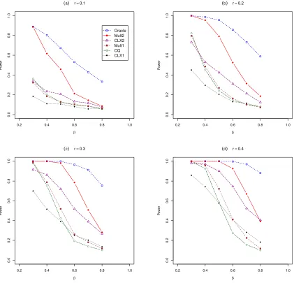
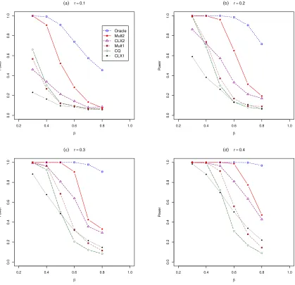
the power profiles of these tests where the powers are displayed with respect to the sparsityβ at four levels of signal strength r= 0.1,0.2,0.3 and 0.4 for Gaussian data. These figures also report the powers of Chen and Qin (2010)’s test (CQ) and the Oracle test to provide some bench marks for the performance.

6. EMPIRICAL STUDY

In this section, we demonstrate the performance of the multi-level thresholding test defined in (4.9) on a human breast cancer dataset, available at http://www.ncbi.nlm. nih.gov. The data have been analyzed by Richardson et al. (2006) to provide insight into the molecular pathogenesis of Sporadic basal-like cancers (BLC), a distinct class of human breast cancers. The original microarray gene expression data consist of 7 normal specimens, 2 BRCA-associated breast cancer specimens, 18 sporadic BLC specimens and 20 non-BLC specimens. Since the most of interests on this data set is to display the unique characteristics of BLC relative to non-BLC specimens, we formed two samples. One consists of n1 = 18 BLC cases and another consists of

n2 = 20 non-BLC specimens for analysis which form two samples respectively.

Biologically speaking, each gene does not function individually in isolation. Rather, genes tend to work collectively to perform their biological functions. Gene-sets are technically defined in Gene Ontology (GO) system that provides structured vocabu-laries which produce names of gene-sets (also called GO terms), see Ashburner et al. (2000) for more details.

As discussed in Richardson et al. (2006), BLC specimens display X chromosome abnormalities in the sense that most of the BLC cases lack markers of a normal inactive X chromosome, which are rare in non-BLC specimens. Moreover, single nucleotide polymorphism array analysis demonstrated loss of heterozygosity (loss of a normal and functional allele at a heterozygous locus) in chromosome 14 and 17 was quite frequent in BLC specimens, a phenomenon largely missing among non-BLC specimens. Therefore, our main interest was on chromosomes X, 14 and 17.

We applied the multi-level thresholding test based on the data transformation on each of gene-sets in chromosomes X, 14 and 17 by first transforming the data with estimated Ω through the Cholesky decomposition discussed in Section 4. We also applied the CQ test to serve as contrasts. By controlling the false discovery rate (Benjamini and Hochberg, 1995) at 0.05, the CQ test declared 81 GO terms significant on chromosome X, 80 out of which were also declared significant by the multi-level thresholding test. However, the multi-thresholding test found 4 more significant GO terms not found significant by the CQ test. Similarly, on chromosome 14, CQ test declared 76 GO terms significant which were all included by the 86 GO terms declared significant by the multi-level thresholding test. On chromosome 17, 5 out of 166 GO terms declared significant by the CQ test were not declared significant by the multi-level thresholding test. On the other hand, 14 out of 175 GO terms declared significant by the multi-level thresholding test were not declared significant by the CQ test.

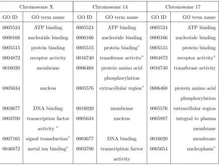
Table 2 lists the top ten most significant GO terms declared by the multi-level thresholding test on the three chromosomes, respectively. The table also marks those gene-sets which were not tested significant by the CQ test. There were three gene-sets in the top ten which were not declared significant by the CQ test in chromosomes X

theoretically findings that the multi-level thresholding test with data transformation is more powerful than the CQ test by conducting both thresholding and utilizing data dependence.

7. DISCUSSION

Our analysis in this paper shows that the thresholding combined with the data trans-formation via the estimated precision matrix leads to a very powerful test procedure. The analysis also shows that thresholding alone is not sufficient in lifting the power when there is sufficient amount of dependence in the covariance, and the data trans-formation is quite crucial. The latter confirms the benefit of the transtrans-formation discovered by Hall and Jin (2010) for the higher criticism test and Cai, Liu and Xia (2014) for the max-norm based test. The proposed test of thresholding with data transformation can be viewed as a significant improvement of the test of Chen and Qin (2010) for sparse and faint signals. The CQ test is similar to the max-norm test without data transformation, except that it is based on the L2 norm.

Gener-ally speaking, the max-norm test works better for more sparse and stronger signals whereas the CQ test is for denser but fainter signals. These aspects were confirmed by our simulations. A reason for the proposed test (with both thresholding and data transformation) having better power than the test of Cai, Liu and Xia (2014) with data transformation is due to the thresholding conducted on the L2 formulation of

the test statistics since the proposed test has both thresholding and data transforma-tion whereas CLX test has only the data transformatransforma-tion. The max-norm formulatransforma-tion does not accommodate the need to threshold. This reveals an adavntage of the L2

formulation.

p-values (Delaigle et al., 2011) is another advantage of the proposal. We want to point out that the study carried out in this paper is not a direct extension from that in Zhong, Chen and Xu (2013). Zhong et al. (2013) considered an alterna-tive L2-formulation to the higher criticism (HC) test of Donoho and Jin (2004) for

one-sample hypotheses. They showed that, although the L2 formulation attains the

same detection boundary as the HC test, the L2 formulation is more advantageous

to the HC when the sparsity and signal strength combination (β, r) is above the de-tection boundary. However, Zhong et al. (2013) did not study the specific benefits of the thresholding in improving the power of the high dimensional multivariate test and the relative performance to the Oracle test; nor did they considered the data transformation via the precision matrix.

APPENDIX: TECHNICAL DETAILS.

Throughout the Appendix, we assume n1 → ∞, n2 → ∞ and let n= _nn₁1₊n_n2₂. A.1. Lemmas

Lemma 1. We denote δk =µ1k−µ2k. As x=o(n

1

3), T_nk in (2.1) satisfies

P(n Tnk+ 1> x) = {1 +o(1)}I(√n|δk|>√x)

+

¯

Φ(√x₋√n_|δk|) + ¯Φ(√x+√n|δk|)

{1 +O(n−1/6)

+ O(x

3/2

n1/2)}I( √

n_|δk|<√x).

Lemma 2. Assume Conditions (C1)-(C2). The mean of the thresholding test statistic Ln(s) is

µLn(s) =

X

i∈Sc β

E_{Ln,i(s)}+

X

k∈Sβ

E_{Ln,k(s)}

=

2

√

2π

p

2slogpp1−s+ X

k∈Sβ

n δ_k2I

n δ_k2 > λn(s)

+ (2slogp) ¯Φ(η_k−)I

n δk2 < λn(s)

Lemma 3. Assume Conditions (C1)-(C3). The variance of the thresholding test statistic Ln(s) is

σ2_Ln(s),1 =

2

√

2π[(2slogp)

3

2 + (2slogp)12]p1−s+ 4pΦ(¯ p2slogp)

+ X

k,l∈Sβ

(4n δkδlρkl+ 2ρ2kl)I

n δ_k2 > λn(s)

I

n δ2_l > λn(s)

+ X

k∈Sβ

(2slogp)2Φ(¯ η−_k)I

n δ2_k < λn(s)

{1 +o(1)_}. (A.2)

Lemma 4. Suppose _{Zi_}p_i=1 is a sequence of α-mixing random variables with zero mean and satisfying

M2l+δ = supi

E(Zi)2l+δ

1/(2l+δ)

<_∞,

for δ >0 and l_≥1. Let α(i) be α-mixing coefficient. Then,

E(

p

X

i=1

Zi)2l_≤Cpl

M₂2_ll+M₂2_ll_+δ

∞

X

i=1

il−1α(i)δ/(2l+δ)

,

where C is a finite constant positive constant depending only on l.

Lemma 5. Under condition (C4), the following relationship holds:

̟kk(τ) =ωkk+O(τ−C), for C >1,

where ωkk={(1−κ)Σ1+κΣ2}−kk1 and ̟kk(τ) = Var{√n( ¯Z1(k)(τ)−Z¯ (k) 2 (τ))}. Lemma 6. If β > 1/2 and the banding parameter τ = Lp for a slowly varying

function Lp, then under condition (C5), with probability approaching 1,

δ_Ω(τ),k ≈ωkkδk for k ∈Sβ,

Lemma 7. For any positive definite matrixAp,p = (aij)p×p and its inverseBp,p =

(bij)p×p, the following inequality holds

Lemma 8. Under the conditions assumed in Theorem 4 and condition (C5), with probability approaching to 1,

β_Jnˆ _(s,τ) ≥βLn(s).

A.2. Proofs of Theorems 1, 2 and 3

The proofs are two-sample extension of Theorems 1, 2 and 3 in Zhong, Chen and Xu (2013). We include them in the supplementary material.

A.3. Proof of Theorem 4

We first derive the mean and variance of the transformed thresholding test statis-tics. Note that by the relationship Zij(τ) = Ω(τ)Xij and

P

l|ωkl|< ∞, for a given

constant C, Z_ij(k)(τ) = P_lωklXij(l)I(|k −l| < τ). Since X

(l)

ij is sub-Gaussian for any

l = 1,_{· · ·} , p, Z_ij(l)(τ) is sub-Gaussian by using H¨older inequality and mathematical

induction. Hence, the large derivation results can be applied to derive the mean and variance of the transformed thresholding test statistic defined in (4.2) by following the similar steps when we derive the mean and variance of the thresholding step. Therefore, to obtain the mean and variance of the transformed thresholding test, we can simply replace δk by δΩ(τ),k and Sβ by SΩ(τ),β in (2.13) and (2.14), respectively,

where after the transformation, nonzero signals δk becomes δΩ(τ),k and the set Sβ

including these nonzero signals becomes S_Ω(τ),β.

We first establish the asymptotic normality of transformed thresholding test de-fined in (4.2) where the banding parametertis chosen to be a slowly varying function. To this end, we first show that both _{Z₁(k_i)(t)_}p_k=1 and _{Z₂(k_i)(t)_}p_k=1 are α-mixing se-quences. By condition (C3), _{X₁(k_j)_}p_k=1 and _{X₂(k_j)_}p_k=1 are α-mixing sequences. Then any event A_∈σ(_FX(1)_,(1,a),_FX(2)_,(1,a)) and B _∈σ(_FX(1)_,(a+k,∞),_FX(2)_,(a+k,∞)),

By the relationship between Z1i(t) and X1i, for any t,

Z₁(a_i)(t)_∈σ(_FX(1)_,(a−t,a+t)), and Z₁(_ia+k)(t)_∈σ(_FX(1)_{,(a+k−t,a+k+t)}).

Then as long as k ₋ 2t _{→ ∞}, _|P(A′ _{∩ B}′_{) − P(A}′_)P(B′_{)| → 0 for any A}′ _∈

σ(_FZ(1)_,(1,a),_FZ(2)_,(1,a)) and B′ _∈σ(_FZ(1)_,(a+k,∞),_FZ(2)_,(a+k,∞)). It follows that

αZ1(t)(k) =αX1(k−2t) if k >2t.

Therefore, αZ1(t)(k) → 0 as k −2t → ∞ where αZ1(t) is the α-mixing coefficient

for the sequence _{Z₁(k_j)(t)_}kp₌₁. Similarly, it can be shown that αZ2(t)(k) → 0 as

k₋2t_{→ ∞}. Thus, both_{Z₁(_ik)(t)_}p_k=1 and_{Z₂(k_i)(t)_}p_k=1 areα-mixing sequences. Then the asymptotic normality of Jn(s, t) can be established by applying the Bernstein’s

blocking method as we have done in the proof of Theorem 1. To further establish the normality of ˆJn(s, τ), we note that our ˆJn can be written as

ˆ

Jn = Jn+ p

X

k=1

(Sˆnk ˆ

ωkk −

Snk

̟kk

)I(Snk

̟kk

> λn) + p

X

k=1

(Snk

̟kk

+ 1)[I(Sˆnk ˆ

ωkk

> λn)

− I(Snk

̟kk

> λn)] + p

X

k=1

(Sˆnk ˆ

ωkk −

Snk

̟kk

)[I(Sˆnk ˆ

ωkk

> λn)−I(

Snk

̟kk

> λn)]

= Jn+ I + II + III,

where ˆSnk =n(Z¯ˆ1(k)−Z¯ˆ (k)

2 )2 andSnk =n( ¯Z1(k)(t)−Z¯ (k)

2 (t))2. To show the asymptotic

normality of ˆJn under H0, we only need to show that I/σJn,0 =op(1) and II/σJn,0 =

op(1) since III is smaller order of I or II.

We first consider I, which can be bounded by

I _≤max1≤k≤p|

ˆ

Snk

ˆ

ωkk −

Snk

̟kk| p

X

k=1

I(Snk

̟kk

> λn).

Using E_{Pp_k=1I(_̟kkSnk > λn)}=Ppk=1P(

Snk

̟kk > λn), and from Lemma 1, p

X

k=1

P(Snk

̟kk

> λn) = O(

p1−s

√

we havePp_k=1I(_̟kkSnk > λn) = Op( p

1−s

√

2slogp). Recall that ˆSnk =n{

P

lωˆkl( ¯X1(l)−X¯ (l) 2 )}2

and Snk =n{P_lωkl(t)( ¯X1(l)−X¯ (l)

2 )}2. Then,

max

k |

ˆ

Snk

ˆ

ωkk −

Snk

̟kk| ≤

max

l n( ¯X

(l) 1 −X¯

(l)

2 )2max_k

(P_lωkl)2

ω2

kk |

ˆ

ωkk−ωkk|{1 +o(1)}

+ max

l n( ¯X

(l) 1 −X¯

(l)

2 )2max

k

P

l|ωkl+

q

ωkk

̟kkωkl(t)|

ωkk

X

l

|ωˆkl−ωkl|

+ X

l

|ωkl−

r

ωkk

̟kk

ωkl(t)|

≤ Mmax

l n( ¯X

(l) 1 −X¯

(l)

2 )2max

k

_Xp

l=1

|ωˆkl−ωkl|+t−a+O(t−C)

,

whereM >0,a >0 and we use the fact that̟kk=ωkk+O(t−C) from Lemma 5. From

the fact that max

l n( ¯X

(l) 1 −X¯

(l)

2 )2 =Op(logp) and maxkPp_l=1|ωˆkl−ωkl|=Op[(logp_n )q/2]

for any q such that 1/(α+ 1)< q <1 (See Bickel and Levina, 2008b), we know

maxk|

ˆ

Snk

ˆ

ωkk −

Snk

̟kk| p

X

k=1

I(Snk

̟kk

> λn) =Op{Lpp1−sn−q/2+ logp(t−a+t−C)},

where Lp and t are slowly varying functions. We can choose t such that logp(t−a+

t−C_{) =o(1). Therefore, we have I =O}

p(Lpp1−sn−q/2). By assumption that p =n1/θ

and s >1₋qθ, then I/σJn,0 =op(1).

For the second term II, we have

II _≤ max

k |

Snk

̟kk

+ 1_|

p

X

k=1

|I(Sˆnk ˆ

ωkk

> λn)−I(

Snk

̟kk

> λn)|

≤ max

k |

Snk

̟kk

+ 1_|max

k I

_ˆ

Snk

ˆ

ωkk

> λn

_Xp

k=1

I

|S_ωˆˆnk

kk −

Snk

̟kk|

>_|Snk ̟kk −

λn|

+ max

k |

Snk

̟kk

+ 1_|maxkI

Snk

̟kk

> λn

_Xp

k=1

I

|_̟Snk

kk −

ˆ

Snk

ˆ

ωkk|

>_|Snk ̟kk −

λn|

:= II1+ II2.

Because the proofs for II1 and II2 are similar, we only show II2 in the following.

First, we note that

max

k |

Snk

̟kk

+ 1_{| ≤} 1 + max

k

(P_lωkl(t))2

̟kk

max

l n( ¯X

(l) 1 −X¯

(l)

And, p X k=1 I

|S_ωˆˆnk

kk −

Snk

̟kk|

>_|Snk ̟kk −

λn(s)|

≤

p

X

k=1

I(_|Sˆnk ˆ

ωkk −

Snk

̟kk|

> h) +

p

X

k=1

I(_|Snk

̟kk −

λn(s)|< h). (A.3)

The second indicator function on the right above can be evaluated by the following:

E

_Xp

k=1

I(_|Snk

̟kk −

λn(s)|< h)

=

p

X

k=1

P(_|Snk

̟kk −

λn(s)|< h)

= p X k=1 ¯

Φ(pλn(s)−h)−Φ(¯

p

λn(s) +h)

= √ h

2slogpp

1−s_.

Therefore, in (A.3), Pp_k=1I(_|̟kkSnk ₋ λn(s)| < h) = Op(√ h

2slogpp

1−s_{). To evaluate}

Pp

k=1I(| ˆ

Snk

ˆ

ωkk − Snk

̟kk|> h) in (A.3), we use the same approach. First, notice that

|Sˆnk

ˆ

ωkk −

Snk

̟kk| ≤

Mmax

l n( ¯X

(l) 1 −X¯

(l) 2 )2

_Xp

l=1

|ωˆkl−ωkl|

+o(1).

Then,

E(

p

X

k=1

I(_|Sˆnk ˆ

ωkk −

Snk

̟kk|

> h))

≤ p X k=1 P Mmax

l n( ¯X

(l) 1 −X¯

(l) 2 )2

p

X

l=1

|ωˆkl−ωkl|> h

≤ p X k=1 P( p X l=1

|ωˆkl−ωkl|>

h M nT2) +

p X k=1 P(max l | ¯

X1(l)−X¯ (l)

2 |> T),

where, if we chooseT =Cplogp/n, Pp_k=1P(max

l |

¯

X₁(l)₋X¯₂(l)_|> T)_≤p2−C _{→0, for}

sufficient large C. If h=C∗logp(log_np)q/2_{, there exists a a >0 such that}

p X k=1 P( p X l=1

|ωˆkl−ωkl|>

h

M nT2) =

p X k=1 P( p X l=1

|ωˆkl−ωkl|> M′(

logp n )

q/2₎

≤p1−a.

Therefore, by choosing C∗ _{large enough such that a > qθ/2,} Pp k=1I(|

ˆ

Snk

ˆ

ωkk − Snk ̟kk| >

Pp k=1I(|

Snk

̟kk−λn(s)|< h) = Op(Lpn− q

2p1−s). In addition, we know that max_kI{Snk

̟kk >

λn(s)}=Op(p−s). Therefore, we know that II2 =op(Lpp1−sn−q/2). Similarly, one can

show that II1 = op(Lpp1−sn−q/2). In summary, II/σJn,0 = op(I/σJn,0) = op(1). This

completes the proof of Theorem 4.

A.4. Proof of Theorem 5

The proof of Theorem 5 is similar to that of Theorem 2. We omit it.

A.5. Proof of Theorem 6

We first consider Ωis known. We know that the power of the transformed thresh-olding test is determined by

SNRJn(s,τ) =

µJn(s,τ),1−µJn(s,τ),0

σJn(s,τ),1

.

Recall that fork_∈Sβ,ωδk2 ≤ δ2

Ω(τ),k ̟kk(τ) ≤ωδ¯

2

k. Then, we have the following inequality

µJn(s,τ),1−µJn(s,τ),0

σJn(s,τ),1 ≥

M1

V1

, (A.4)

where M1 = P

k∈Sβ

nωδ2

kI(nωδk2 >2slogp) + (2slogp) ¯Φ(ηk−)I(nωδk2 <2slogp)

and

V₁2 = _√2

2π{(2slogp)

3

2 + (2slogp)12}p1−s

+ X

k,l∈Sβ

(4nω2δkδlρΩ,kl+ 2ρ2_Ω,kl)I(nωδ2k>2slogp)I(nωδl2 >2slogp)

+ X

k∈Sβ

(2slogp)2Φ(¯ η_k−)I(nωδ_k2 <2slogp).

Note that M1/V1 is the signal-to-noise ratio of the thresholding test without the

transformation. But the signal nωδ2

k = 2ωrlogp. From the proof of Theorem 3, we

know that M1/V1 → ∞ as long as s is properly chosen and ωr > ̺(β). Therefore,

µJn(s,τ),1−µJn(s,τ),0

σJn(s,τ),1 → ∞

,

To show the second statement in part (a) of Theorem 6, we notice that the maximal transformed thresholding test is of asymptotic α level. Therefore, it is sufficient to show that its power tends to 1 above the detection boundary as n _{→ ∞} and α_→0. To this end, we notice that

P(MJn ≥Gα|H1) ≥ P

_J

n(s, τ)−µJn(s,τ),0

σJn(s,τ),0 ≥

Gα|H1

= Φ

− σJn(s,τ),0

σJn(s,τ),1

Gα+

µJn(s,τ),1−µJn(s,τ),0

σJn(s,τ),1

≥ Φ

− σJn(s,τ),0

σJn(s,τ),1

Gα+

M1

V1

.

Then, we can choose αn = ¯Φ{(logp)ǫ} → 0 as p → ∞ for any small number ǫ > 0

such that Gα =O{(loglogp)1/2}. If ωr > ̺(β), we can find as satisfying one of cases

given in the proof of Theorem 3 such that the second term in Φ(_·) dominates and tends to infinity, which leads to Φ(_·)_→1.

Then we consider the first statement in part (a) of Theorem 6. Note that

µJn(s,τ),1−µJn(s,τ),0

σJn(s,τ),1 ≤

M2

V2

,

where M2 = P

k∈Sβ

nωδ¯ 2

kI(nωδ¯ k2 >2slogp) + (2slogp) ¯Φ(ηk−)I(nωδ¯ k2 <2slogp)

and

V₂2 = √2

2π{(2slogp)

3

2 + (2slogp) 1 2}p1−s

+ X

k,l∈Sβ

(4nω¯2δkδlρΩ,kl+ 2ρ2_Ω,kl)I(nωδ¯ 2k>2slogp)I(nωδ¯ l2 >2slogp)

+ X

k∈Sβ

(2slogp)2Φ(¯ η_k−)I(nωδ¯ _k2 <2slogp).

We also note that M2/V2 is the signal-to-noise ratio of the thresholding test with

nωδ¯ 2

k = 2¯ωrlogp, which converges to 0 for any s if ¯ωr < ̺(β), i.e.,

µJn(s,τ),1−µJn(s,τ),0

σJn(s,τ),1 →

0.

Similar to the proof for the second statement of Theorem 3, we can show that

where ˜Jn(s) = (Jn(s)−µJn(s,τ),1)/σJn(s,τ),1. Since

P_{a(logp) max

s∈Tn

˜

Jn(s)−b(logp, c)≤x} →exp(−e−x),

where c = max(η₋r+ 2r√1₋η₋β, η)I(r < 1₋η) + max(1₋β, η)I(r > 1₋η). Then, similar to the proof in Theorem 3, we have

P(MJn ≥Gα|H1) =α{1 +o(1)} →0,

which implies that the type II error tends to 1 as α_→0. Next we consider Ω is unknown. Let G⋆

α = {qα +b(logp, η⋆ −θ)}/a(logp). If

we choose αn = ¯Φ{(logp)ǫ} → 0 as p → ∞ for any small number ǫ > 0, G⋆α =

O_{(loglogp)1/2_{}. We only show that if r > ω}−1_̺

θ(β), the sum of type I and II of M_Jnˆ

converges to 0, since the proof that the sum of type I and II of M_Jnˆ tends to 1 if

r <ω¯−1_̺

θ(β) is similar to the proof for MJn. We notice that

P(M_Jnˆ ≥G⋆α|H1) ≥ P

_ˆ

Jn(s, τ)−µˆJn(s,τ),0

ˆ

σJn(s,τ),0 ≥

G⋆_α|H1

= P

_J

n(s, τ)−µJn(s,τ),0

σJn(s,τ),0

+µJn(s,τ),0−µˆJn(s,τ),0

σJn(s,τ),0

+ op(1)

σJn(s,τ),0

ˆ

σJn(s,τ),0 ≥

G⋆_α|H1

, (A.5)

where we have used the fact that ifp=n1/θ_{for 0< θ <1, ( ˆJ}

n(s, τ)−µJn(s,τ),0)/σJn(s,τ),0

= (Jn(s, τ)−µJn(s,τ),0)/σJn(s,τ),0+op(1) given in the proof of Theorem 5. Moreover,

as shown in Zhong, Chen and Xu (2013), with p=n1/θ _{for 0< θ <1,}

µJn(s,τ),0−µˆJn(s,τ),0

σJn(s,τ),0 →

0, and σJn(s,τ),0 ˆ

σJn(s,τ),0 →

1.

Then the probability in (A.5) is determined by

Jn(s, τ)−µJn(s,τ),0

G⋆

ασJn(s,τ),0

=

Jn(s, τ)−µJn(s,τ),1

G⋆

ασJn(s,τ),1

+ µJn(s,τ),1−µJn(s,τ),0

G⋆

ασJn(s,τ),1

σJn(s,τ),1

σJn(s,τ),0

,

where (Jn(s, τ)−µJn(s,τ),1)/(G⋆ασJn(s,τ),1) = op(1), andσJn(s,τ),1 > σJn(s,τ),0. Therefore,

inequality (A.4), we only need to show that with properly chosen s, M1/(G⋆αV1) → ∞. As we have shown in Theorem 5, we need to choose the level of the threshold

s_∈(1₋θ,1) if Ωis unknown such that the asymptotic normality of the transformed thresholding test with ˆΩ can be established. The modification on the detection boundary can be derived by adding the additional restriction s > 1₋θ on the four cases in the proof of Theorem 3. Similar to the result in Delaigle, Hall and Jin (2011), and Zhong, Chen and Xu (2013), the modified detection boundary is given by (4.11). As a result, we know that M1/(G⋆αV1) → ∞ if ωr > ̺θ(β). This shows

that if r > ω−1_̺

θ(β), the power of M_Jnˆ tends to 1.

REFERENCE

Ashburner, M., Ball, C., Blake, J., Botstein, D., Butler, H., Cherry,

J., Davis, A., Dolinski, K., Dwight, S., Eppig, J., Harris, M., Hill, D.,

Issel-Tarver, L., Kasarskis, A., Lewis, S., Matese, J., Richardson, J.,

Ringwald, M., Rubin, G. and Sherlock, G. (2000). Gene ontology: tool for

the unification of biology. Nature Genetics,25, 25-29.

Bai, Z. and Saranadasa, H. (1996). Effect of high dimension: by an example of

a two sample problem. Statistic Sinica, 6, 311-329.

Benjamini, Y. and Hochberg, Y. (1995). Controlling the false discovery rate: A

practical and powerful approach to multiple testing. Journal of the Royal Statis-tical Society: Series B,57 289-300.

Bickel, P. and Levina, E. (2008a). Regularized estimation of large covariance

matrices. The Annals of Statistics, 36, 199-227.

Bickel, P. and Levina, E. (2008b). Covariance regularization by thresholding.

The Annals of Statistics, 36, 2577-2604.