Munich Personal RePEc Archive
State Ownership and Corruption
Billon, Steve and Gillanders, Robert
April 2014
Online at
https://mpra.ub.uni-muenchen.de/55600/
öMmföäflsäafaäsflassflassflas
fffffffffffffffffffffffffffffffffff
Discussion Papers
State Ownership and Corruption
Steve Billon
Aalto University and HECER
and
Robert Gillanders
Aalto University and HECER
Discussion Paper No. 378
April 2014
ISSN 1795-0562
HECER
Discussion Paper No. 378
State Ownership and Corruption*
Abstract
Using data from the World Bank's Enterprise Surveys, we test two interesting results that
emerge from the theoretical model presented in Shleifer and Vishny (1994) that studies
bargaining between politicians and managers of state-owned firms. Shleifer and Vishny's
model suggests that firms with more state ownership should tend to pay less in bribes but
not have a different experience of costly obstacles imposed on them by politicians. In our
full sample, the results suggest that a one percent increase in state ownership is
associated with a $125 reduction in the total annual informal payment of the firm and with
a 0.5% decrease in the probability that a firm will consider corruption to be an obstacle to
their current operations. We refine these average relationships somewhat by splitting the
sample by global region. Only in our Europe and Central Asia sample do we find strong
evidence in support of the first result and in this sample we find a signifcant effect of state
ownership on obstacles. In our Sub-Saharan Africa and Latin America and Caribbean
samples we do not find a significant effect on either corruption outcome.
JEL Classification:
D73, G32, L32, L33, P31
Keywords:
state ownership, corruption, privatisation, bribery
Steve Billon
Robert Gillanders
Department of Economics
Department of Economics
Aalto University
Aalto University
P.O. Box 21240
P.O. Box 21240
FI-00076 AALTO
FI-00076 AALTO
FINLAND
FINLAND
e-mail:
[email protected]
e-mail:
[email protected]
1
Introduction
In the traditional public finance approach, the intervention of the state is often seen as an efficient cure to solve market failures such as the inadequate provision of public goods or the presence of externalities in the consumption or in the production of a private good. In this view, the objectives of politicians who influence public enterprises are in line with those of the general public and state-owned enterprises help to maximise social welfare as they internalise the social cost in the decision process of production, yielding an efficient outcome. In contrast, Shleifer (1998) argues that self-interested politicians exchange votes from political supporters for benefits to these particular interest groups or directly extract bribes from the state-owned enterprise, so that state ownership leads to inefficiency and corruption.
Empirically, the literature suggests that a reallocation of ownership in state-owned en-terprises in favour of private ownership does not seem to lead to less corruption non-ambiguously. For instance, Kaufmann and Siegelbaum (1997) highlight that the experience of sharp privatisation in the transition economies of the Former Soviet Union (FSU) and Central and Eastern Europe (CEE) were accompanied by a substantial increase in the per-ception of corruption as well as the relative importance of the unofficial economy. However, they argue that it is possible to design optimal programs of privatisation that reduce the opportunities for corruption by government officials.
Few models have been developed to analyse theoretically the relationship between the own-ership structure of enterprises and corruption. Bjorvatn and Soreide (2005) stress a link between market concentration and corruption that works in two ways. On the one hand, the search for rent extraction may lead politicians to strategically sell a public enterprise to one enterprise that will obtain a monopoly position. The rational behind such behaviour is that it maximises the acquisition price of a state-owned enterprise. On the other hand, the acquiring firm in the post-privatized economy may benefit from its newly monopolistic position to engage in corruption in order to secure its advantage. In this case, privatisation leads to more corruption through a greater concentration of the privatised market.
to an increase in the level of bribes. However, the level of obstacles imposed does not change with state ownership.
We then bring these theoretical results to the data. For this purpose we use the World Bank’s Enterprise Survey (WBES) which provides detailed information at the firm level. We are especially interested in the firms’ experience of corruption, measured both in terms of bribe amounts and the degree to which they feel corruption is an obstacle to their operations. Our results show that not only the presence of the state in the ownership of a firm but also the degree of the state ownership has a negative, statistically significant and economically mean-ingful relationship with both the amount of bribes paid and the probability that corruption is seen as an obstacle by a firm. In regional sub-samples, we find that the relationship is particularly relevant in Europe and Central Asia but not for Sub-Saharan Africa and Latin America.
Several papers have looked empirically at the effect of privatisation on corruption. Fan et al. (2009), who focus on the relationship between decentralisation and corruption, find that state ownership decreases corruption. However, their state ownership measure is mainly used as a control variable and the only information to which they have access is thepresence of the state in the capital of the firm, represented by a dummy variable coded as 1 if any state agency or state body has a financial stake in the ownership of the firm and 0 otherwise. In contrast, we introduce a finer measure of state ownership since we use the percentage of the firm that is owned by the state. This measure gives information not only on the presence but also on thestrength of this presence in the ownership of the firms. Analysing the 1999 Business Environment and Enterprise Survey, Hellman et al. (2000) report that the frequency of bribe payment as well as the average amount of bribes paid is higher for new private firms compared to privatised and state owned enterprises. Arikan (2008) shows that privatisation in the form of lower employment share of state economic enterprises fosters the perception of corruption. This result is present in a sample of transition economies as well as in general and is robust to different privatisation indicators.
to previous studies, their results exhibit a negative effect of all privatisation variables on corruption. Note that most of these papers only look at the effect of the type of firms (de novo, privatised, state-owned) or some proxy measure of privatisation on corruption. In contrast, our state ownership variable allows us to consider a continuum of firms from fully private to fully state-owned and to analyse the effect of marginal changes in ownership structure on corruption.
The paper is organised as follows. Section 2 presents a simplified version of the Shleifer and Vishny (1994) model and derives the main hypotheses regarding the link between state ownership and corruption. Section 3 presents the data and the methodology used to test this relationship. Section 4 presents the results and Section 5 concludes by discussing some policy implications.
2
Theory
The model of Shleifer and Vishny (1994) describes the relationship between the public, a politician and a firm’s manager. The capital of the firm is owned in partκ∈[0,1] by the Treasury and in part (1−κ) by the manager and shareholders. The manager is assumed to follow the objectives of the shareholders. Let π be the profit (assumed to be strictly positive) of the firm before it interacts with the politician. Transfers between the politician and the manager may occur in two ways: either from the politician to the manager in the form of a subsidiest financed by the Treasury, or from the manager to the politician in the form of a bribe. Thus Shleifer and Vishny (1994) envision several channels by which the politicians might influence and corrupt firms managers. The politicians use a transfer from the Treasury to firms with two objectives in mind. The first one is to partly finance obstacles they impose on firms and that bring back a political benefit to them. These obstacles may take the form of excess employment, as argued by Shleifer and Vishny (1994). For instance, the government and the beneficiaries of this excess employment such as politically influential labour unions may engage in a political market in which votes are exchanged for jobs, as described by the public choice school. These obstacles may also take the form of regulations (Svensson; 2003) or influence the production of goods in favour of the politician and his political supporters at the expense of the general public. Second, bribes are a way for the politicians to appropriate part of the public funds coming from the Treasury in the form of transfers as well as some of the firm’s profit.
T =t−κ(t−O)
= (1−κ)t+κO, (1)
where O represents the obstacles the politician imposes on the manager. The net transfer incurs a cost δ(T) on the politician, reflecting the political constraint of using the public funds of the Treasury for his own interest. On the other hand, the politician enjoys a benefit
γ(O) from the obstacles he imposes on the firm (γ′(O)>0). Note thatO, in contrast to the bribe, does not fall in the politician’s pocket in the form of money. These obstacles might be for example the employment of individuals that will favor his reelection as in Shleifer and Vishny (1994). O could also capture politicians obliging managers to purchase other (possibly inferior) non-labour inputs from sources beneficial to the politician. The utility of the politician is given by:
Up=γ(O)−δ(T) +b, (2)
whereb is the amount of bribes paid and the utility of the manager reads:
Um= (1−κ)(π+t−O)−b
= (1−κ)π+T−O−b. (3)
(3) is found by substituting (1) in the utility of the manager. Note that the bribe, as an informal payment, is not divided between the private and public shareholders (Treasury) of the firm but is entirely borne by the manager (who is equivalent to the private shareholders in this model).
We now turn to the objective and strategic variables of the politician. In contrast to Shleifer and Vishny (1994) who allow the control right over the obstacles O to be devoted either to the politician or to the firm, we assume that the choice over O is always under the control of the politician. We focus on this case to make clear the effect of a change in the ownership structure on bothband O. Thus the politician sets the level of obstacles O, the net transfer T and the bribeb in order to maximize his utility (2) subject to the positive utility participation constraint of the manager: (1−κ)π+T −O−b ≥ 0. The relevant Lagrangian for this problem reads:
ℓ=γ(O)−δ(T) +b+λ{(1−κ)π+T−O−b}, (4)
∂ℓ ∂T =−δ
′(T) +λ= 0, (5a)
∂ℓ ∂O =γ
′(O)−λ= 0, (5b)
∂ℓ
∂b = 1−λ= 0, (5c)
∂ℓ
∂λ = (1−κ)π+T −O−b= 0. (5d)
Simplifying yields:
γ′(O) =δ′(T) = 1. (6)
The condition (6) may be viewed as two separate conditions over O andT. It means that the politician extracts the maximum amount of transfers from the Treasury so as to finance increases in the obstacles on firms that politically benefit to him. However the politician has to balance the benefits of these obstacles with a political cost which occurs because of possible sanction for the use of public funds for private interests, for instance in terms of decreasing probability of being reelected. The transfer extraction from the Treasury continues until the marginal political benefit of the obstacles is equal to the marginal political cost of the net transfer. Then the politician extracts the bribe from the utility of the manager by pushing him to zero net profit.
Totally differentiating the optimal condition on the net transfer from the Treasury (i.e.
δ′(T) = 1), we can show, by substituting (5d), the effect of change in the degree of public
ownership in the enterprise on the level of the bribe:
∂b
∂κ =−π <0. (7)
(7) indicates that an increase in the public ownership of the firm leads to a decrease in the bribe imposed by the politician. The rationale behind this result is that a higher public ownership drops the profit (1−κ)πof the firm and thus the potential rent the politician is able to extract from the manager. IfO andT are constant, then a increase inκimplies a lower bribe payment in order to keep (5d) unchanged. Differentiating the manager’s participation constraint (5d), we also show that:
∂O
∂κ =−π− ∂b
∂κ = 0, (8)
compensate any deviation from this equilibrium, as we can see in the second term of the RHS of (8). In the case where there are too little obstacles, the politician compensates the manager by giving up bribes in order to increase obstacles up to the optimal level. If the obstacles are too great, the manager compensates the politician by paying bribes in order to reduce the obstacles to the optimal level.
3
Data
3.1
The Enterprise Surveys
To test the predictions of the Shleifer and Vishny (1994) model outlined above, namely that state ownership reduces the amount paid in bribes by a firm and has no effect on the degree to which corruption is an obstacle to a firm’s operations, we need measures of these two outcomes. Until relatively recently such finely grained information on corruption was hard to come by, especially if one desired internationally comparable data for a wide range of countries. Recently however, the World Bank’s Enterprise Surveys and similar projects have begun to document firms’ (self reported) experiences of corruption. The Enterprise Surveys are representative firm level surveys that have been carried out in an increasing number of developing and emerging economies as well as some more developed economies. They provide a wide range of information on firms’ characteristics, the business environment they operate in, and the constraints they face, be they legal, political or other. The dataset we use contains over 55000 firm level observations from 105 countries though the sample size we can use is dictated primarily by our choice of dependent variable. The full methodology is available at the Enterprise Surveys website.1
3.2
Corruption Measures
To measure the amount of bribes paid, we make use of the following question:
We’ve heard that establishments are sometimes required to make gifts or informal payments to public officials to “get things done” with regard to customs, taxes, licenses, regulations, services etc. On average, what percent of total annual sales, or estimated total annual value, do establishments like this one pay in informal payments or gifts to public officials for this purpose?
Note that the question refers to “establishments like this” in order to help elicit truthful responses. We use the data for those who chose to give the response in terms of total annual informal payment rather than as a percent of total annual sales and refer to this asbribe.
1
We focus on this quantity for two main reasons. Firstly, the theory says nothing about the quantitybribe/sales. Secondly, when we look at the data we can see that the vast majority of non-zero responses to the bribe/sales question are multiples of 5. This suggests that respondents were prone to rounding off their guess as to what the actual value was.2
Our second dependent variable is derived from a survey question that asks respondents if corruption is no obstacle, a minor obstacle, a major obstacle, or a very severe obstacle to the current operations of their establishment. From this we create a dummy variable,Obstacle, that takes a value of one if the firm feels that corruption is a major or very severe obstacle and zero otherwise. This is our measure ofO, the obstacles placed in the way of the firm by the politician in the model above. Given that thisO can be many different things as argued above, the simplicity and openness of this question are desirable features.
3.3
State Ownership
Our explanatory variable of interest comes from a survey question that asks what percent-age of the firm is owned by private domestic entities, private foreign entities, the govern-ment/state, and “others”. From this we create a dummy variable that takes a value of one if the state has any ownership in the firm in line with Fan et al. (2009). However we also use the continuous nature of the variable. Thus we will be examining whether firms with
any state ownership have lesser corruption problems than those that do not and likewise, and more in keeping with the theory, if firms withmore state ownership do. Using a con-tinuous variable also allows us to see if the relationship is non-linear - a possibility that the theoretical model does not consider.
We drop 13 observations. These 13 firms all reported total annual informal payments in excess of one million dollars (the next highest was roughly $800,000) and had reported current or past sales that were either extremely high, equal to the reported bribe payment, or greater than it. Including these 13 firms (12 from Sub-Saharan Africa and one from Latin America) does not alter the findings in terms of the statistical significance of our main result but greatly inflates the estimated relationships in the full sample and the Sub-Saharan Africa sub-sample.
2
When we do usebribe/sales as our dependent variable we find no relationship with state ownership and it does not even predict whetherbribe/saleswas non-zero in probit models. Further, if we create a new variable for bribe amount by multiplyingbribe/sales by our variable measuring sales we fail to find a relationship with state ownership. We also fail to find a relationship when we create a newbribe/sales
3.4
Summary Statistics
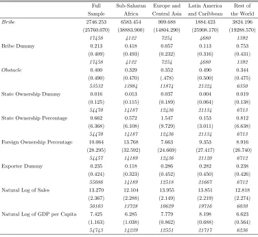
Table 1 reports summary statistics for all the variables used in this paper. All variables bar the data on GDP per capita data come from the Enterprise Surveys. The GDP per capita variable comes from the World Development Indicators. All monetary responses from the survey data have been adjusted for prices and converted to US dollars. We also report the summary statistics for the sub-samples of Sub-Saharan Africa (SSA), Europe and Central Asia (ECA), Latin America and Caribbean (LCA) and Rest of the World (ROW). The average firm pays $2746 in informal payments per year though this varies substantially, both in terms of standard deviations and in terms of global region. Roughly 20% of firms have had to pay at least something in bribes though again this varys across the globe with 42% of firms in SSA paying a bribe and only 6% of firms in our ECA sample and 11% in our LCA sample doing so.
However when we look at theObstaclevariable we can see that the story is somewhat dif-ferent with 40% of firms overall feeling that corruption is an obstacle to their operations. The number is still high when we look at the ECA sample and is comparable to the SSA value while the LCA sample displays a substantially higher value. Whether this is due to different modalities of corruption manifesting differently in different (general) environments or is due to a propensity to over or under “complain” about corruption is an open question. Corruption could be a hinderance to firms beyond bribes as outlined above and even firms that are not involved in corruption may feel it is a problem if it helps their rivals to succeed, discourages investment from abroad (e.g. Wei (2000a), Wei (2000b), and Habib and Zuraw-icki (2002)) lowers the quality of infrastrucutre (e.g. Tanzi and Davoodi (1997), Bose et al. (2008), and Gillanders (2014)) or leads to one of the other myriad problems identified in the corruption literature. This difference between the relative levels of each variable certainly reinforces the need to look at both measures beyond the theoretical motivation and assertion that both are important and distinct modalities of corruption.
Table 1: Summary Statistics
Full Sub-Saharan Europe and Latin America Rest of Sample Africa Central Asia and Caribbean the World
Bribe 2746.253 6583.454 909.688 1884.423 3824.196 (25760.070) (38883.900) (14804.290) (25908.170) (19288.570)
17458 4132 7254 4680 1392
Bribe Dummy 0.213 0.418 0.057 0.113 0.753
(0.409) (0.493) (0.232) (0.316) (0.431)
17458 4132 7254 4680 1392
Obstacle 0.400 0.329 0.352 0.490 0.344
(0.490) (0.470) (.478) (0.500) (0.475)
53532 13984 11874 21324 6350
State Ownership Dummy 0.016 0.013 0.037 0.004 0.019
(0.125) (0.115) (0.189) (0.064) (0.138)
54470 14187 12436 21134 6713
State Ownership Percentage 0.662 0.572 1.547 0.153 0.812
(6.368) (6.108) (9.729) (3.011) (6.638)
54470 14187 12436 21134 6713
Foreign Ownership Percentage 10.064 13.768 7.663 9.353 8.916 (28.295) (32.592) (24.669) (27.417) (26.740)
54457 14189 12436 21120 6712
Exporter Dummy 0.235 0.118 0.286 0.282 0.238
(0.424) (0.323) (0.452) (0.450) (0.426)
55086 14189 12518 21667 6712
Natural Log of Sales 13.270 12.104 13.955 13.851 12.818
(2.367) (2.288) (2.149) (2.219) (2.274)
50103 13728 10629 19716 6030
Natural Log of GDP per Capita 7.425 6.285 7.779 8.198 6.623 (1.163) (1.038) (0.862) (0.688) (0.564)
54743 14239 12551 21717 6236
Notes: The first entries in the table are means. Standard deviations are given in parentheses and the number of observations is in
4
Empirical Specification and Results
4.1
Empirical Specification
To test the theoretical predictions regarding the responses ofb and O to a change in κwe estimate models of the following form:
bribei=α0+β1SOW Ni+β2F OW Ni+β3EXPi+β4SALESi+β5GDP P Ci+ǫi (9)
P r(obstaclei= 1) = Φ(ζ1SOW Ni+ζ2F OW Ni+ζ3EXPi+ζ4SALESi+ζ5GDP P Ci+νi)
(10)
where the former is estimated by OLS and the later is a probit model. bribei and obstaclei
are our measures ofband O respectively. It must be noted that since this measure of O is discrete rather than continuous we do not have a direct test of ∂O∂κ. However it seems logical
to assume that there is a positive relationship between the level of O and the probability that it is seen as a serious problem. We refine this somewhat by using an ordered probit model as a robustness test. SOW Ni is our measure ofκ, the degree of state ownership in
the firm. ǫi andνi are error terms of the usual type.
We control for several factors suggested by our intuition and by the existing literature. First we control for the degree of foreign ownershipF OW Ni as such firms may stand in different
relation to bureaucrats than others, could be more or less willing (and able) to pay bribes, and may present a more guilt-free target to officials. Firms that export may come into contact with more, and different, officials and so we include a dummy (EXPi) that takes a
value of one if some of the firm’s sales are not national sales. Like Fan et al. (2009) we control for the size of the firm using the natural logarithm of sales (SALESi). If we use dummies
for the size of the firm in terms of number of employees we obtain the same results. Finally we control for the level of GDP per capita (GDP P Ci) in the firm’s country in line with
the long standing literature that has found that GDP per capita is a significant factor in determining perceptions of corruption. Good examples of this finding are Ades and Di Tella (1999), and Svensson (2005). This may help to deal somewhat with the potential for some cultures at certain stages of the development process to be more prone to “complaining” about corruption than others.
errors with our splits, the only important difference is thatbribeis significant at 5% in our SSA sample as opposed to 10%.
4.2
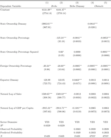
Basic Results
Table 2 presents our main results. Column 1 shows that having any degree of state ownership lowers the total annual informal payment by almost $4000. This is clearly an economically meaningful quantity and the result is highly statistically significant. Turning to Column 2, we can see that when we refine this by using the continuous nature of the data we still find a highly statistically significant and economically meaningful result. Each percentage of state ownership lowers the bribe paid by about $125. We find only slight evidence of a non-linear effect. The squared term is positive though of negligible estimated size and is only significant at 10%. The results suggest that a firm with 10% state ownership will pay roughly $1250 less in bribes per year than similar firms while an entirely state owned firm will pay $12500 less. These sums, while not astronomical, are unlikely to be inconsequential for most firms. The theoretical prediction of Shleifer and Vishny (1994) that the bribes paid by firms should decrease with the level of state ownership seems to hold true in general, though as we will soon see it does not appear to hold in every environment.
Foreign ownership operates similarly to state ownership though to a smaller degree. Each percentage of foreign ownership tends to reduce the annual bribe burden by around $20, a small but statistically significant amount. This is worth contrasting with Fan et al. (2009) who found that any foreign ownership significantly decreased the frequency of bribery but not the amount (as a percentage of sales, categorically measured). Larger firms tend to pay significantly and substantially more in bribes whereas the opposite is true for firms in richer countries.
There are clearly concerns one might have with self-reported bribe information. One ro-bustness check we can run is to discard most of the information and simply look at whether state ownership predicts that at least some amount is paid in bribes. We can see in Column 3 that each percentage of state ownership reduces the probability of having to pay anything in bribes by about 0.4%. While this may seem small at first, it is a statistically significant result and implies that a firm with 10% state ownership is 4% less likely to have to pay any bribes at all relative to similar firms with no state ownership. Certainly, it is an effect that dwarves that of foreign ownership. In this specification we find a role for exporter status with exporters being nearly 5% more likely to have to pay a bribe. Larger firms are no more or less likely to pay a bribe though firms in richer countries are less likely to do so.
Table 2: Main Results
(1) (2) (3) (4) (5)
Dependent Variable: Bribe Bribe Dummy Obstacle
Constant 6121.39∗∗ 6101.37∗∗
(2754.14) (2753.14)
State Ownership Dummy -3992.01∗∗∗ -0.0844∗∗∗
(967.91) (0.0201)
State Ownership Percentage -125.24∗∗∗ -0.0041∗∗ -0.0053∗∗∗
(35.18) (0.0019) (0.0015)
State Ownership Percentage Squared 0.66∗ 0.0000 0.0001∗∗∗
(0.35) (0.0000) (0.0000)
Foreign Ownership Percentage -20.24∗∗ -20.60∗∗ -0.0005∗∗ -0.0005∗∗∗ -0.0005∗∗∗
(9.98) (10.04) (0.0002) (0.0001) (0.0001)
Exporter Dummy 128.99 122.95 0.0463∗∗∗ 0.0013 0.0014
(723.75) (724.43) (0.0171) (0.0091) (0.0091)
Natural Log of Sales 1569.65∗∗∗ 1569.82∗∗∗ -0.0012 0.0003 0.0004
(308.58) (308.77) (0.0034) (0.0022) (0.0022)
Natural Log of GDP per Capita -2915.31∗∗ -2914.71∗∗∗ -0.1481∗∗∗ 0.0065 0.0064
(597.63) (598.06) (0.0119) (0.0073) (0.0073)
Sector Dummies YES YES YES YES YES
R2
0.0229 0.0229
Observed Probability 0.2363 0.3928 0.3928
Predicted Probability 0.1929 0.3923 0.3923
N 15428 15428 15428 47557 47557
Notes: Columns 1 and 2 report OLS coefficients. Columns 3, 4 and 5 report probit marginal effects. Standard errors are clustered at
tend to be around 8% less likely to feel that corruption is an obstacle to their operations. Once again this is an economically meaningful result and is highly statistically significant. However this empricial result is in contradiction with the theoretical model presented above that predicts that there is no relationship between obstacles and onwnership. However, this contradiction is explicable if we consider that the theoretical result relies on the Coase theorm.
A well known critique of the Coase theorem is that it may not apply if many contracting agents (in our case the politicians or the managers) have to agree on a compensation scheme to reach the optimal level of obstacles. Suppose that state ownership uniformly decreases in every firm. In order for the incentive compatibility constraint to hold, obstacles should decrease (holdingb constant). Following the Coase theorem, the managers should pay more bribes in order to come back to the optimal level of obstacles. But if there are many managers, any individual player finds himself ia a classical prisoner’s dilemma. It is his interest to free ride on the compensation scheme and to let the other managers agree to a level of bribe payment in order to obtain less obstacles. This is because he will benefit from the decrease in obstacles without paying for it. As a consequence, no bribe compensation will emerge to counteract the negative effect ofκonO and the second term, db/dκ, in the RHS of (8) will vanish. The same argument applies if there are too little obstacles and many politicians on the political market. In these conditions, it is not surprising to find this result that contradicts the ideal case of the model where there is only one politician and one manager.
The final column shows that this result holds when using the continuous measure of state ownership. As mentioned above, this is not a direct test of the theoretical prediction as we do not have a continuous measure ofObut it seems logical to assume that there is a strong link between the levelO and the probability of it being seen as an obstacle. Thus we have empirical evidence that, contrary to the prediction of the Shleifer and Vishny (1994) model, more state ownership decreases the obstacles placed in the way of the firm by corruption.3
We also allowed for the possibility that this relationship is non-linear by including a squared state ownership term. It seems plausible that while certain levels of state ownership may shield firms from corruption, extreme levels of state ownership may make a firm the readily exploitable fiefdom of certain officials. On the other hand, extreme levels of state ownership could perhaps reinforce the beneficial effect. The results suggest that the former is true though this non-linear effect is not very large relative to the effect of the level of state ownership. Foreign ownership also matters though once again it matters to a much lesser degree than state ownership. The other variables are all insignificant.
3
As argued by Shleifer (1998), the level of corruption in a society might have an influence on the structure of ownership. In particular, a highly corrupt government might be less willing to privatise. In other words, state ownership and corruption may be endogenous. Unfortunately, we lack suitable variables that we could use as instruments for state ownership in the current context. Indeed it is difficult to think of what such instruments could be. However, the nature of our data on corruption make us confident about our results: while it is plausible the overall level of corruption influences the state ownership policy, it is less likely that individual firms’ experiences of corruption directly have such effect.4
Further, the model of Shleifer and Vishny (1994) on which we are basing our analysis provides a strong, logical and, we feel, convincing argument for the existence of a clear causal mechanism through which the degree of state ownership helps determine a firm’s experience of corruption.
4.3
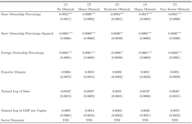
Extensions
To get somewhat closer to the theoretical quantity Oand to provide a sensible robust test, we made use of the full range of information provided by the survey question from which we createdObstacle. Table 3 presents the results of this exercise. More state ownership is associated with a lower probability of a firm feeling that corruption is a moderate, major, or very severe obstacle to their operations and a higher probability of feeling that is is no obstacle or a minor obstacle. Thus we can conclude that our findings with regards to
Obstacleare not the result of the specific way we use the data.
The conclusions one can draw often vary dramatically by the global region under consid-eration. Certain regions have tended to have different experiences of state ownership. It is generally good practice to split ones sample by broad geographical region and it makes particular sense to do so in the context of state ownership and corruption. For example, the former Soviet states and satellites that can be found in our ECA sample will tend to have had very different histories of state ownership and control than the countries in our other samples. Similarly, corruption and general institutional malaise is more common and severe in Sub-Saharan Africa than in other regions of the globe. Corruption may be so endemic in these countries that the theoretical mechanisms outlined above may be irrelevant.
Table 4 presents the results of our two specifications run on our 4 groups of countries. Only in the ECA sample do we see strong evidence in favour of the theoretical hypothesis regardingbribe. The magnitude of the relationship between bribes paid and state ownership is considerably smaller than in the full sample at $50 but it is highly significant as is the squared term. The findings in terms ofObstacleare quite similar to those in the full sample. In SSA, we find no strong evidence of either relationship. We suspect that this is due to the pervasive nature of corruption in SSA. That said, as the state ownership variable
4
Table 3: Ordered Probit Marginal Effects for Corruption as an Obstacle
(1) (2) (3) (4) (5)
No Obstacle Minor Obstacle Moderate Obstacle Major Obstacle Very Severe Obstacle State Ownership Percentage 0.0052∗∗∗ 0.0008∗∗∗ -0.0002∗∗∗ -0.0017∗∗∗ -0.0041∗∗∗
(0.0011) (0.0002) (0.0001) (0.0003) (0.0009)
State Ownership Percentage Squared -0.0001∗∗∗ 0.0000∗∗∗ 0.0000∗∗ 0.0000∗∗∗ 0.0000∗∗∗
(0.0000) (0.0000) (0.0000) (0.0000) (0.0000)
Foreign Ownership Percentage 0.0004∗∗∗ 0.0001∗∗∗ -0.0000∗∗ -0.0001∗∗∗ -0.0003∗∗∗
(0.0001) (0.0000) (0.0000) (0.0000) (0.0001)
Exporter Dummy -0.0064 -0.0010 0.0002 0.0021 0.0051
(0.0072) (0.0012) (0.0002) (0.0023) (0.0059)
Natural Log of Sales -0.0032∗ -0.0005∗ 0.0001 0.0010∗ 0.0026∗
(0.0019) (0.0003) (0.0001) (0.0006) (0.0015)
Natural Log of GDP per Capita -0.0091 -0.0014 0.0003 0.0030 0.0073
(0.0065) (0.0010) (0.0002) (0.0021) (0.0052)
Sector Dummies YES YES YES YES YES
Notes: Ordered Probit Marginal Effects. Standard errors are clustered at the country-sector level and are reported in parentheses.∗,
Table 4: Sample Splits by Global Region
(1) (2) (3) (4) (5) (6) (7) (8)
Global Region: Sub-Saharan Europe and Latin America Rest of
Africa Central Asia and Caribbean the World
Dependent Variable: Bribe Obstacle Bribe Obstacle Bribe Obstacle Bribe Obstacle
Constant -26926.00∗∗∗ -2448.57 -1364.91 -39264.17∗∗∗
(6968.57) (1660.12) (6394.32) (11517.30)
State Ownership Percentage -430.13∗ 0.0040∗ -49.60∗∗∗ -0.0062∗∗∗ 220.56 -0.0056 -61.34 -0.0133∗∗∗
(241.15) (0.0023) (15.30) (0.0018) (298.36) (0.0036) (93.40) (0.0032)
State Ownership Percentage Squared 1.24 -0.0001∗ 0.39∗∗ 0.0001∗∗∗ -2.49 0.0000 0.06 0.0001∗∗∗
(2.55) (0.0000) (0.15) (0.0000) (3.07) (0.0000) (1.18) (0.0000)
Foreign Ownership Percentage -103.83∗∗∗ -0.0002 -9.84∗ -0.0007∗∗∗ -6.04 -0.0003∗∗ 12.13 -0.0009∗∗∗
(26.11) (0.0001) (5.40) (0.0002) (11.73) (0.0001) (39.30) (0.0003)
Exporter Dummy 4024.89 0.0264∗ 134.05 -0.0188 732.66 0.0082 1978.81 0.0166
(3069.01) (0.0139) (559.61) (0.0119) (957.88) (0.0090) (1496.98) (0.0185)
Natural Log of Sales 5184.20∗∗∗ 0.0142∗∗∗ 314.56∗∗∗ -0.0005 592.59∗∗∗ -0.0111∗∗∗ 1046.13∗∗ -0.0019
(719.55) (0.0021) (95.24) (0.0026) (159.44) (0.0019) (478.36) (0.0034)
Natural Log of GDP per Capita -4033.39∗∗∗ -0.0237∗∗∗ -112.48 -0.0675∗∗∗ 184.83 -0.1241∗∗∗ 4463.01∗ -0.0730∗∗∗
(553.79) (0.0041) (204.85) (0.0060) (454.30) (0.0056) (2285.90) (0.0131)
Sector Dummies YES YES YES YES YES YES YES YES
R2
0.0800 0.0050 0.0094 0.06
Observed Probability 0.3243 0.3412 0.4878 0.3257
Predicted Probability 0.3227 0.3383 0.4876 0.3212
N 4026 13437 6081 10008 3942 18831 1379 5281
Notes: Columns where “Bribe” is the dependent variable report OLS coefficients. Columns where “Obstacle” is the dependent variable
report probit marginal effects. Robust standard errors in parentheses. ∗,∗∗and∗∗∗indicate significance at the 10%, 5% and 1%
is significant at 10% and the magnitude of the association with bribe is rather large and negative, policymakers thinking about privitisation or reducing corruption in SSA may be interested in these results, though the association withObstacleis positive. In LAC we don’t see any evidence of either relationship and in the RoW sample we only find a relationship withObstacle, though this is a rather small and heterogeneous sample.
Finally, we looked for specific ways in which state ownership might make corruption less of an obstacle for firms. We failed to find any relationship between the degree of state ownership and the probability of having to pay a bribe in the specific circumstances of obtaining a construction permit, during tax inspections, obtaining an operating license, or with the percentage of a government contract that must be paid in informal gifts in order to secure the contract. At the macro level Breen and Gillanders (2012) found that the level of corruption in a country was a determinant of the ease of doing business in that country. However, we also failed to find a relationship between state ownership and bureaucratic constraints such as the days it takes for imports and exports to clear customs, time spent dealing with government regulations, losses due to crime, and the probability of the firm finding any of the following to be an obstacle to their operations: tax administration, the courts, obtaining business licenses and permits, zoning, and customs. Once again these findings, full results of which are available on request, stand somewhat in contrast with those of Fan et al. (2009) who found a link between their state ownership dummy and the frequency of bribery for purposes of business licenses, tax collection, government contracts, public utilities, customs, and the courts. We tentatively propose that these results suggest that theObstaclevariable is capturing the outcomes of machine type politics (e.g. “jobs for the boys”).
5
Conclusions
Using data from the World Bank’s Enterprise Surveys we have found partial empirical sup-port for the theoretical predictions of the model presented in Shleifer and Vishny (1994). The percentage of state ownership in a firm significantly and substantially decreases the amount of bribes that the firm has to pay and reduces the probability that corruption is seen as an obstacle to the firm’s operations. The second result, while not consistent with the prediction the model, is easily explained by free-riding incentives that invalidate the Coase theorem. Specifically, we found in our baseline estimation that each additional one percent-age of state ownership reduces the total annual informal payment by $125 and decreases by about 0.5% the probability that a firm will consider corruption to be an obstacle to their current operations. As one might expect, there is substantial regional heterogeneity.
Asia, who are concerned about reducing corruption may wish to reconsider their attitudes to privatisation. We have shown that any degree of state involvement in ownership is beneficial in terms of a firm’s experiences of corruption. Of course we are not saying that privatisation is a bad policy. Though Birdsall and Nellis (2003) argue that privatisation is perhaps not a good policy in terms of equality, there is a long standing literature that tends to conclude that privatisation is good in terms of efficiency. Eckel et al. (1997) show this in the specific case of the privatisation of British Airways and Megginson and Netter (2001) and Estrin et al. (2009) provide good overviews of this literature. Gupta (2005) shows that even partial privatisation has a positive effect on firm performance.
References
Ades, A. and Di Tella, R. (1999). Rents, competition, and corruption, American economic review89(4): 982–993.
Arikan, G. G. (2008). How privatizations affect the level of perceived corruption, Public Finance Review36(6): 706–727.
Birdsall, N. and Nellis, J. (2003). Winners and losers: Assessing the distributional impact of privatization,World Development31(10): 1617–1633.
Bjorvatn, K. and Soreide, T. (2005). Corruption and privatization, European Journal of Political Economy21(4): 903–914.
Bose, N., Capasso, S. and Murshid, A. (2008). Threshold effects of corruption: Theory and evidence,World Development36(7): 1173–1191.
Boubakri, N., Cosset, J. P. and Smaoui, H. (2009). Does privatization foster changes in the quality of legal institutions?,Journal of Financial Research32(2): 169–197.
Breen, M. and Gillanders, R. (2012). Corruption, institutions and regulation,Economics of Governance13(3): 263–285.
Clarke, G. R. G. and Xu, L. C. (2004). Privatization, competition, and corruption: How characteristics of bribe takers and payers affect bribes to utilities,Journal of Public Eco-nomics88(9-10): 2067–2097.
Eckel, C., Eckel, D. and Singal, V. (1997). Privatization and efficiency: Industry effects of the sale of british airways,Journal of Financial Economics43(2): 275–298.
Estrin, S., Hanousek, J., Koˇcenda, E. and Svejnar, J. (2009). The effects of privatization and ownership in transition economies,Journal of Economic Literature47(3): 699–728.
Fan, C., Simon Lin, C. and Treisman, D. (2009). Political decentralization and corruption: Evidence from around the world,Journal of Public Economics93(1-2): 14–34.
Gillanders, R. (2014). Corruption and infrastructure at the country and regional level,
Journal of Development Studies. forthcoming.
URL:http://www.tandfonline.com/doi/abs/10.1080/00220388.2013.858126
Gupta, N. (2005). Partial privatization and firm performance, The Journal of Finance
60(2): 987–1015.
Hellman, J. S., Jones, G., Schankerman, M. and Kaufmann, D. (2000). Measuring gover-nance, corruption and state capture: How firms and bureaucrats shape the business envi-ronment in transition economies,Policy research working paper 2312, The World Bank.
Kaufmann, D. and Siegelbaum, P. (1997). Privatisation and corruption in transition economies,Journal of International Affairs50(2): 419–458.
Koyuncu, C., Ozturkler, H. and Yilmaz, R. (2010). Privatization and corruption in transition economies: A panel study,Journal of Economic Policy Reform13(3): 277–284.
Megginson, W. L. and Netter, J. M. (2001). From state to market: A survey of empirical studies on privatization,Journal of Economic Literature39(2): 321–389.
Shleifer, A. (1998). State versus private ownership, Journal of Economic Perspectives
12(4): 133–150.
Shleifer, A. and Vishny, R. W. (1994). Politicians and firms,Quarterly Journal of Economics
109(4): 995–1025.
Svensson, J. (2003). Who must pay bribes and how much? Evidence from a cross section of firms,Quarterly Journal of Economics118(1): 207–230.
Svensson, J. (2005). Eight questions about corruption,The Journal of Economic Perspectives
19(3): 19–42.
Tanzi, V. and Davoodi, H. (1997). Corruption, public investment, and growth,IMF Working Paper WP/97/139, IMF.
Wei, S.-J. (2000a). How taxing is corruption on international investors?,Review of economics and statistics82(1): 1–11.