Philippine Export Efficiency and
Potential: An Application of Stochastic
Frontier Gravity Model
Deluna, Roperto Jr and Cruz, Edgardo
University of Southeastern Philippines, School of Applied Economics
February 2014
Online at
https://mpra.ub.uni-muenchen.de/53580/
Roperto S. Deluna Jr1
ABSTRACT
This study was conducted to investigate the issue of what Philippine merchandise trade flows would be if countries operated at the frontier using gravity model. The study sought to estimate the coefficients of the gravity equation. The estimated coefficients were used to estimate merchandise export potentials and technical efficiency of each country in the sample and these were also aggregated to measure impact of country groups.
Result of the estimated coefficients of the gravity equation shows that merchandise export flows of the Philippines to trading partners is significantly positively affected by income and market size of the importing partner. The income elasticity of merchandise exports is 0.69%. A 1% increase in market size increases export flow by 0.24%. Distance was estimated to reduce export flow by 1.22% in every 1% increase in distance.
The technical efficiency for all sample countries is not so high; it ranged from 38 to 42% with standard deviation of 30. The most efficient countries in the sample which recorded more than 80% efficiency were Singapore (100%), New Zealand (97%), HongKong (97%), USA (96%), Australia (96%), Canada (96%), UK (93%), Denmark (93%), Japan (87%), Malaysia (85%) and S. Korea (81%). Countries with larger markets emerge as high export potentials such as USA, China and Japan with potential ranging from 10 to 30 Trillion US dollars.
These potential has been changing within the period. Result of technical inefficiency model reveals that these potential is increased by membership of the Philippines to ASEAN, APEC and WTO. Reduction of corruption and freer labor market in the importing country enhances export potential of Philippine merchandise exports. Commonality of language also enhances these potential.
Keywords: Merchandise exports, Gravity, Stochastic frontier, Philippine export potential
1
INTRODUCTION
Trade is the exchange of goods and services across regions and national
borders was considered important in improving welfare of people even before the birth
of economics as organized science in 1776. The mercantilist philosophy maintained that
the way for a nation to be rich and powerful was to export more than to import. The Philippines is one of the world‟s oldest open economies, which traded goods even prior to its discovery by the western world. For more than a century however, it experienced
widening gap between exports and imports which causes trade deficit. This means that
the country is not trading at its potential, which may be due to its institutional and
infrastructures rigidities or the rigidities of its trading partner which will be explored in
this study.
Transactions of the Philippines with the rest of the world are recorded in the Balance of Payment (BOP) which shows country‟s external economic position. The BOP is composed of current, capital and financial account. Figure 1 shows a positive
BOP position of the Philippines since 2004 which reflects a positve extenal position.
This means that financial inflow to the Philippines is greater than outflow to the rest of
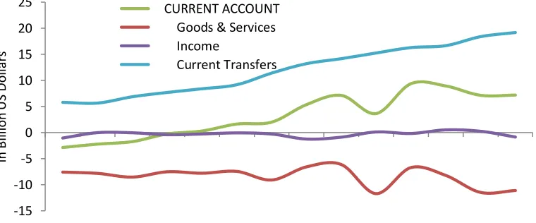
the world. Current account as one of the components of the BOP shows the flows of
goods and services, income and current transfers. It was observed that the Philippines
have been operating a current account surplus since 2003 (pushing the BOP), despite a
large trade deficit as reflected in Figure 2. Current account surplus stimulates domestic
production and income while the deficit dampens domestic production and income.
This surplus in the current account is accounted to current transfers and strong
remittances inflows of Overseas Filipino Workers (OFW) which are represented as
income. Moreover, trade of goods and services pulls current account surplus. This
Figure 1. Balance of payment (BOP), Philippines, 1999-2012.
Source of Data: Philippine Institute of Development Studies http://econdb.pids.gov.ph/tablelists/table/153
Figure 2.Current account balance, Philippines, 1999-2012.
Source of Data: Philippine Institute of Development Studies http://econdb.pids.gov.ph/tablelists/table/153
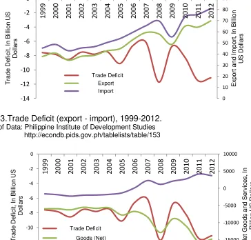
Trade deficit is an economic measure of a negative balance of trade in which a
country's import exceeds its export (Figure 3) which was observed in the Philippines for
decades. Figure 4 show that huge trade deficit was accounted to large deficit on traded
goods. A trade deficit represents an outflow of domestic currency to foreign markets.
Furthermore, it causes the strengthening of foreign currency against the home currency
which results in expensive importation of goods and services as compared to -4
-2 0 2 4 6 8 10 12 14 16
1999 2000 2001 2002 2003 2004 2005 2006 2007 2008 2009 2010 2011 2012
In
B
il
li
o
n
US
D
o
ll
ar
s
Overall BOP Position
Current Account
Capital and Financial Account
Net Unclassified Items
-15 -10 -5 0 5 10 15 20 25
1999 2000 2001 2002 2003 2004 2005 2006 2007 2008 2009 2010 2011 2012
in
B
il
li
o
n
US
D
o
ll
ar
s
CURRENT ACCOUNT Goods & Services Income
[image:4.612.120.500.331.489.2]exportation home-produced goods and services.These are the impacts of devalued
[image:5.612.114.464.128.283.2]home currency (peso) and if significantly large can cause BOP deficit.
Figure 3.Trade Deficit (export - import), 1999-2012.
[image:5.612.109.473.134.482.2]Source of Data: Philippine Institute of Development Studies http://econdb.pids.gov.ph/tablelists/table/153
Figure 4.Trade Deficit (goods + services), 1999-2012.
Source of Data: Philippine Institute of Development Studies http://econdb.pids.gov.ph/tablelists/table/153
The characteristics of exports and global trade are radically changing as the
world recovers from the recent global financial crisis and the natural disasters in Japan.
Moreover, the unfolding political events in the Middle East and North Africa (MENA) will
contributed to volatile market conditions. The key features are the speedy growth of
emerging economies with large consumer populations and the sluggish single-digit
growth of developed markets. This will result in the re-balancing of consumption, export
market size and supply chain configurations in relation to pre-crises periods (PEDP,
2011-2013).
These changes in global export environment pose opportunities for the
Philippines to grow exports of merchandise and services. This leads the Philippines to
target a forty percent (+40%) increase in export by 2013 and to exceed Philippine
exports by one hundred twenty billion U.S dollars (US$ 120B) by 2016 as targeted in
the Philippine Export Development Plan (PEDP). The 2016 target is more than twice
compared to the 2012 Philippine export value of US$ 57.5B (BSP Database).
Achievement of this target requires understanding of the factors that prevent the
Philippines to reach its export potential. These factors could be explored to achieve the
target of PEDP.
Conventional trade study uses Gravity Model to explain trade flows between two countries as directly proportional to the product of each country‟s „economic mass‟ that can be measured by their Gross Domestic Product (GDP) and inversely proportional to
the distance between the countries (Anderson, 1979). This model was derived from
different theories but was criticized because of weak theoretical foundations. This is
rectified the recent work to the point where Frankel, Stein and Wei (1997) claimed that the gravity model has “gone from an embarrassing poverty of theoretical foundation to an embarrassment of riches” as cited by Armstrong (1997). This model was very successful in analyzing trade flows. However, this cannot provide estimates of trade
potential if estimated using the Ordinary Least Square (OLS) regression analysis as the
commonly used method in estimating conventional gravity models.
Earlier studies have estimated the difference between observed values and the
estimated predicted values by using the gravity equation through OLS estimates as
potential trade (Baldwin, 1994 and Nilsson, 2000) between a pair of countries. The OLS
estimation procedure produces estimates that represent the centered values of the data
set. However, potential trade refers to free trade with no restrictions to trade. Thus, for
policy purposes, it is rational to define potential trade as a maximum possible trade that
can occur between any two countries, which has liberalized trade restrictions the most,
given the determinants of trade. This means that the estimation of the potential trade
values of the data (Kalirajan, 2007). To address this, the concept of stochastic
production frontier analysis which deals with the upper bound of the data set to measure
the maximum possible output is utilized (Drysdale et al., 2000).
This thesis is an attempt to investigate the trade patterns and constraints of the
merchandise exports of the Philippines using the gravity stochastic frontier model. It
seeks to analyze factors affecting trade of merchandise export. It also aims to come up
with technical efficiency estimates for each of the trading partner. Further, the study
attempt to assess if multilateral agreements of the Philippines increase the volume of
Philippine trade.The factors considered in this study are “beyond the border” constraints
and natural constraints to trade. This will also estimate export potential and compare it
with actual export performance to see whether there are still some opportunities to
ensure the surplus of the current account of the balance of payments by increasing the
volume of exported goods. Estimation of the model will follow the proposed method of
Drysdale et al., (2003) and Kalirajan and Finley (2005). The study includes comprehensive measures of “beyond the border” constraints which are product of recently established country specific indices which are not included in the studies in the
literatures.
Knowing the trade potential and factors affecting it could narrow down trade
deficit especially in merchandise export. Narrowing the trade deficit is an advantage of
the country as it will be reflected in a trade surplus of current account balance. The
surplus of the current account of BOP is a full factor for the Philippines to achieve an
investment grade sovereign rating which boost capital inflows and positive factor for the
Philippines Economic fundamentals like appreciation of Philippines peso against US
dollars.
Understanding the rigidities that affect export flows could help policy maker‟s
efforts to minimize or at least mitigate the effects of existing restrictive measures of
trade growth, i.e., engaging in bilateral and multilateral agreements and processes.
Therefore the objective of every country is to try to achieve its full trade potential
through the engagement process or even through unilateral reforms. It is of significant
regions in order to get the engagement process started. Enhancement of this trade
flows will enhance welfare of people.
OBJECTIVES OF THE STUDY
This study aims to analyze the export flows between the Philippines from 2009 to
2012 based on 69 trading partners of merchandise exports. Specifically, the study
aims:
1. to estimate the potential trade between the Philippines and its trading partners;
2. to estimate the technical efficiency of Philippine merchandise exports to each
trading partners; and,
3. to determine the constraints to Philippine trade.
THE GRAVITY MODEL
The Gravity Model is based on the law of universal gravitation in physics
developed by Isaac Newton in 1687 which described the gravitational force between
two masses in relation to the distance that lies between them (Newton, 1687), that is
The gravitational force is proportional to the product of the two masses and and inversely proportional to the square of the distance that keeps the two masses apart from each other. The gravitational constant G is an empirical determined value.
This relationship is applicable to any context where the modeling of flows or movements
is demanded (Starck, 2012).
The gravity equation was first applied to international trade flows by Timbergen in
1962. He assumed the relationship as in equation 1.
There is a direct proportionality between the explanatory variables and the variable to
elasticity of the importing country‟s GDP () and the elasticity of distance (). Where,
==1 and =2, in equation 2, will correspond to the universal gravitation equation of Isaac Newton. By taking the natural logarithm of equation 2 and by adding the error
term a linear relationship is obtained. This is traditionally estimated using the Ordinary Least Squares (OLS) regression analysis; the coefficients can be interpreted
as elasticities.
( ) ( ) ( )
Anderson (1979) was one of the first economists who developed a sound
theoretical foundation of the gravity model that brought gravity model into mainstream
economics. The development of the Anderson‟s theoretical foundation of gravity model
was gradual. His work became the basic theoretical framework for a gravity model of
trade flows with the basic assumptions of homothetic preferences for trade goods
across countries and using the constant elasticity of substitution (CES) preferences.
Anderson yielded the specification of aggregated trade flows as final gravity
equation
∑
[∑ ]
Adding the error term , equation 4 can be rewritten as
∑
[∑∑ ]
where,
= Exports of country to country
= Income in country
= Distance between country and country
= The share of expenditure on all traded goods and services in total
Inherent Bias of the Gravity Model
According to Anderson (1979), the log linear of equation 5 resembles the
standard gravity equation in equation 3, with an important difference. This difference is
the bracket term in equation 5 which is:
[∑∑
]
This is missing in the generally used empirical specification of the gravity model
presented in equation 4. Anderson (1979) described this term as “the flow from to
depends on economic distance from to relative to a trade weighted average of
economic distance from to to all points in the system. Measuring the correct
specification of the relative economic distance term is difficult because researchers do
not know all the factors affecting this term. The economic distance can be affected by
many factors, including institutional, regulatory, cultural and political, which are difficult to measure completely. These factors are referred to as „behind the border‟ constraints of the importing countries or constraints to export.
Omission of this term in the empirical work of gravity model leads to the biasness
of the estimation. This is because the term in the square brackets (economic distance
term) of equation 18 affects the log-normal distribution of the error term. Therefore, the expected value of the error term is no longer zero (E(Uij) ≠ 0) and the normality assumption of OLS is violated. This omission leads to heteroskedastic error terms and
the log-linearization of the empirical model in the presence of heteroskedasticity leads
to inconsistent estimates because the expected value of the logarithm of a random
variable depends on higher-order moments of its distribution (Silva and Tenreyro, 2003
as cited in Miankhel et al., 2009). Therefore, the OLS estimation on such gravity
equations will be biased.
Aside from the violation of the OLS normality assumption, the estimation of these
conventional gravity models through OLS provides the values at the mean of the
observation or sample countries. This is problematic in determining trade potential
stochastic production frontier analysis was incorporated to the gravity model. In this
case, export potential is conceptually similar to a firm producing at the frontier.
STOCHASTIC FRONTIER GRAVITY MODEL
The Gravity Stochastic Frontier Model is the Integration of Gravity Model and
Stochastic Frontier Production Function Model which was formally introduced by
Kalirajan (2000) to address the inherent bias of the conventional gravity model of trade
and to estimate potential trade flows.
With a stochastic frontier approach, the gravity equation can be written as:
( )
where the term represents the actual exports from country to country . The term ( ) is a function of the determinants of potential trade and is a vector of
unknown parameters. The single sided error term, is the economic distance bias
referred by Anderson (1979), which is due to the influence of the “behind the border measures” of the importing country. This bias creates the difference between actual and potential trade between two countries. takes value between 0 and 1 and it is usually assumed to follow a truncated (at 0) normal distribution, .
When takes the value 0, this indicates that the bias or country-specific “behind the border constraints” are not important and the actual exports and potential exports are
the same, assuming there are no statistical errors. When take the value other than 0 (but less than or equal to 1), this indicates that the bias or country-specific “behind the border” constraints are important and they constrain the actual exports from reaching potential exports. The double-sided error term , which is usually assumed to be
, captures the influence on trade flows of other left out variables, including
measurement error that are randomly distributed across observations in the sample.
Export potential is conceptually similar to a firm producing at the frontier. When a
firm is producing at the frontier, it has achieved economic efficiency which is composed
when a country achieves its trade potential or is trading at the frontier, the country is
trading in the most efficient manner. Export potentialis defined as the export achieved
when there is least resistance (least inefficiencies) to trade given the current trade,
transport and institutional practices (Drysdale et. al., 2000; Kalirajan, 2000; Armstrong,
2007). In other words, export potential is explained as the maximum possible value of
exports that could hypothetically be attained using the most open (most efficient) trade
policies observed.Following from this argument, we can define export performance (the
achieved export efficiency of the economy) as the ratio of actual to potential exports as
shown in equation 7.
( )
( )
The advantages of the suggested method of estimation of the gravity model are
as follows: Firstly, it does not suffer from loss of estimation efficiency. Secondly, it
corrects for the economic distance bias term, which is creating heteroskedasticity and
non-normality, isolating it from the statistical error term. This isolation property will enable us to examine how effective are the importing countries “behind the border constraints” as major trade constraints. Thirdly, the suggested approach provides potential trade estimates that are closer to frictionless trade estimates. This is because
the approach represents the upper limits of the data, which come from, those
economies that have liberalized their trade restrictions the most (Miankhel, et al., 2009).
Finally, the suggested method bears strong theoretical and trade policy implications
towards finding ways of minimizing unilateral impacts to volume of trade.
CONCEPTUAL FRAMEWORK OF THE STUDY
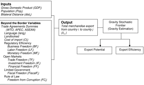
The flow of the study and variables are presented in Figure 8. The study will
utilize secondary data from various sources to estimate the stochastic frontier gravity
model and determine the export potential of the Philippines to trading partners. The
model will utilize GDP, population and bilateral distance between country to . Since
the study will employ the stochastic frontier gravity model which is similar to estimation
variables like trade agreements between Philippines and partner country; commonality
[image:13.612.57.555.142.435.2]of language, landlocked, and partner country specific measures was explored.
Figure 5. Estimation framework of stochastic frontier gravity model.
DATA SOURCES
This study utilized panel data consisting of 69 bilateral trading partners of the
Philippines on merchandise exports from 2009 to 2012. The list of countries included in
this study is shown in Table 1 which was chosen based on their relative importance to
Philippine merchandise exports. The aggregate data on merchandise export was taken
from the Department of Trade and Industry (DTI). Data on Gross Domestic product as
proxy to income and population as proxy for market size was taken from the World
Bank. Data on bilateral distance measured in kilometers, landlocked, language and
land area was secured from the Centre d'Etudes Prospectives et d'Informations
Internationales (CEPII)whichwas developed by Mayer and Zignago (2005).
Beyond the Border Variables
Trade Agreements Dummies (WTO, APEC, ASEAN) Language (langj)
Landlocked Cost of import (CIj)
Regulatory Efficiency
Business Freedom (BFj) Labor Freedom (LFj) Monetary Freedom (MFj)
Open Markets
Trade Freedom (TFj) Investment Freedom (IFj) Financial Freedom (FFj) Limited Government
Fiscal Freedon (FiscalFj) Rule of Law
Freedom from Corruption (FCj)
Output
Total merchandise export from country to county ( )
Export Potential
Gravity Stochastic Frontier (Gravity Estimation)
Export Efficiency
Inputs
Gross Domestic Product (GDPj) Population (Popj)
Table 1. Trade partners (69) of Philippine merchandise exports to be included in the study.
AFRICA (6) UAE Sweden
Algeria Viet Nam Switzerland
Egypt Yemen UK
Kenya EUROPE (25) Ukraine
Madagascar Austria NORTH AMERICA (7)
South Africa Belgium Canada
Tunisia Croatia Costa Rica
ASIA (20) Cyprus Dominican Republic
Bangladesh Denmark Guatemala
Cambodia Finland Mexico
China France Panama
Hongkong Germany USA
India Greece SOUTH AMERICA (7)
Indonesia Hungary Argentina
Japan Italy Brazil
Jordan Lithuania Chile
S. Korea Luxembourg Colombia
Lebanon Netherlands Ecuador
Macau Norway Peru
Malaysia Poland Uruguay
Nepal Portugal OCEANIA (4)
Saudi Arabia Russia Australia
Singapore Slovak Republic Micronesia
Sri Lanka Slovenia Papua New Guinea
Thailand Spain New Zealand
Note: Classification is based from http://www.worldatlas.com/cntycont.htm#.Ugv73aCHMag
“Beyond the Border” variables including freedom from corruption (FC), fiscal freedom (FiscalF), business freedom (BF), labor freedom (LF), monetary freedom (MF),
trade freedom (TF) investment freedom (IF) and financial freedom (FF) was taken from
the Heritage Foundation. List of APEC member countries was taken from apec.org
while ASEAN member countries were taken from asean.org. World Trade Organization
EMPIRICAL APPLICATION
Adopting the methodology proposed by Drysdale et.al. (2000) and Kalirajan and
Finley (2005), the stochastic frontier approach of the gravity model in equation 6,
imposing the variables proposed in this study can be rewritten as:
where:
- is the total value of exports from Philippines (i) to partner country (j)
at time t.
- Gross Domestic Product of country j at time t as proxy for income. - population of country j as proxy for market size.
- is the geographical distance between the capital cities of country i
and j measured in kilometers.
- Single sided error for the combined effects of inherent economic
distance bias or „behind the border‟ constraints, which is specific to the exporting country with respect to the particular importing country, creating the difference between actual and potential bilateral trade. is assumed to have an iid nonnegative half normal distribution that is
– Double sided error term that captures the impact of inadvertently
omitted variables and measurement errors that are randomly
distributed across observations in the sample. is assumed to follow an iid normal distribution with mean zero and constant
variance that is .
The disturbance term can be specified as:
The inefficiency effect model,are specified in equation 9 captures significant
factors that contribute to Philippine merchandise export inefficiency.
where:
- is a dummy variable that takes the value of 1 if country j is a member of Association of Southeast Nation and 0, otherwise. -is a dummy variable that takes the value of 1 if country j is a
member of World Trade Organization and 0, otherwise.
- is a dummy variable, 1 if country js‟ language is English and 0 otherwise.
- is a dummy variable, 1 if the country j is landlocked and 0
otherwise.
- cost of importing , this measures the fees levied on a 20-foot container on to import goods in U.S. dollars..
- Trade Freedom index of country j, which is a composite measure of the absence of tariff and non tariff barriers in partner country j which includes quantity, price, regulatory, investment, customs restrictions and direct government intervention. The TF score of each partner country j is a number between 0 and 100.The higher the score implies lesser barriers of trade.
- is Business Freedom index developed by The Heritage Foundation, is an overall indicator of the efficiency of government regulations of business. The BF score of each partner country j is a number between 0 and 100 with 100 as the freest business environment. - Investment Freedom Index of partner country j determines how free
the flow of investment capital is. The higher the score, the freer is the investment into and out of specific activities, both internally and across the country‟s border. The IF score of each partner country j is a number between 0 and 100with 100 as the freest in terms of investment.
-Freedom from corruption index of country j developed by
Transparency International‟s Corruption Perception Index (CPI). The FC score of each partner country j is a number between 0 and 100, the higher the score indicates little corruption.
- is Fiscal Freedom index of country j, is a measure of the tax
burden imposed by the government, it includes direct taxes on individuals and corporate incomes. The index lies between 0 to 100, the higher the index means the higher tax burden.
- Labor Freedom index of country j, measures various aspect labor market‟s legal and regulatory framework including minimum wages, laws inhibiting layoffs, severance of requirements and measurable regulatory restraints on hiring and hours worked. The index lies between 0 to 100, the higher the index means freer labor.
–Financial Freedom index of country j, is a measure of banking
efficiency as well as a measure of independence from government control and interference in the financial sector. The index lies between 0 to 100, the higher the index means higher financial freedom.
ESTIMATION
The estimation of equations 23 and 24 was done simultaneously using Frontier 4.1
software of Tim Coelli (2004). Frontier follows the Kumbhakar and McGuckin
(1991) and Reifschneider and Stevenson (1991) idea to estimates all of the parameters
in one step procedure to be consistent on the assumption that inefficiencies are
independently and identically distributed (iid).
RESULTS
Philippine Merchandise Exports
Figure 6 presents trend of merchandise exports from 1948 to 2012 in the
Philippines. The general trend of merchandise exports within the period is rising,
however, at generally fluctuating growth rates.
The Philippines trade policies from 1950‟s to the late 1960‟s focused on imports
and were generally protectionist in nature. In 1950‟s, the country adopted
import-substitution policies mainly to conserve scarce foreign currency assets in the central
bank rather than as a long-term development framework (Power and Sicat, 1970). This regime of protectionism resulted to “profit incentive which evoked a strong entrepreneurial response; and what began as an emergency tactic became the principal
policy instrument for promoting industrialization in the 1950's (Power and Sicat, 1970).
In the 1960‟s, the government begun to decontrol import and foreign exchange
markets. A tariff structure was set in place in 1962 under the Macapagal Administration
(Sicat, 2002) that preserved the same industrial structure that had been protected by
the earlier import/exchange control structure. The highest tariff rates were set on
structure would remain essentially unchanged until the early 1970‟s (Power and
Sicat 1970).
Trade policy changes were introduced in 1970‟s targeted export oriented
industries and created the Board of Investments (BOI), and the 1970 Export
Incentives Act (RA 6135), which specified the qualifications of a domestic
industry to receive tax exemptions and subsidies on imports, and expanded the
list of qualified industries and businesses. It was also at this stage that economic
diplomacy entered into the picture through the creation of Association of
Southeast Asian Nations (ASEAN) in 1967. This has lead to high growth rates
of merchandise exports from 1970 to 1974. It reached a peak of 71% in 1973.
This can also be attributed to a world price commodity boom in the same period
and the devaluations of the Philippine currency (Bautista, et al., 1979). The
Organization of Petroleum Exporting Countries (OPEC) oil crises during this
period, however, wiped out most of these gains in manufacturing, including the
1973 trade surplus. This caused severe downturn on export growth rates until
1975, which recovered minimally in 1976 to 1979. The brewing political and economic crisis in the late 1970‟s and early 1980‟s as the impact of martial law hampered the growth of the export sectors. The sector was able to recover after
the political transition in 1986.
Export growth was stable from 1986 to 1999, when the economy
recovered from the extreme political instability. Philippine exports was
surprisingly unaffected by the 1997 Asian financial crisis which secured a growth
rate of 21% and continued to rise until 1999. This growth rate was not maintained
and dipped to an all time low of -18% in 2001, the ousting of President J. E.
Estrada.
The earlier part of 21st century recorded low export growth rates. In response, the government under Executive Order No. 554 of 2006, eliminated
fees and charges on export clearances, inspections, permits, certificates and
other documentation requirements, except those imposed by specific laws or
Figure 6. Philippine merchandise exports (ME), 1948-2012.
Source of data: World Bank Database
Regime of protectionism
New tariff structure
ASEAN
OPEC Oil Crisis
Pol. Crisis (Martial Law)
Pol. Transition (EDSA)
Recovery
Asian Crisis
Pol. Crisis (Estrada) E.O. 554
World Financial Crisis Export stimulus fund
(40)
(20)
20
40
60
0.20
0.40
0.60
0.80
1.00
1.20
1948
1951
1954
1957
1960
1963
1966
1969
1972
1975
1978
1981
1984
1987
1990
1993
1996
1999
2002
2005
2008
2011
A
n
n
u
al
g
ro
w
th
r
a
te
(
%
)
Me
rc
h
an
d
is
e
E
xp
o
rt
s
in
B
il
li
o
n
US
growth rate surge to 15% in 2006. This was not maintained, when the country‟s
export sector was strongly hit by the world financial crisis in 2007. In response,
the government allotted an economic stimulus fund to provide financial
assistance to exporters which was lifted when the sector recovered in 2010. The
export sector recovered and peaked at 33%. This was not maintained, growth
rate was fluctuating until 2012. The average growth rate from 1948 to 2012 was
10%.
Figure 7 shows that manufactures dominated merchandise export in the
Philippines. This is followed by machinery and transport equipment, office and
[image:20.612.114.495.457.683.2]telecom equipment, and integrated circuits and electronic components.
Figure 8 shows the global markets of Philippine merchandise exports from
2007 to 2012. Japan is the most important market which imports around 11% to
20% from 2007 to 2012. This is higher compared to the total exports of the
Philippines to major regional trading blocs such as ASEAN, European Union
(EU) and North America Free Trade Agreement (NAFTA). This is followed by
China, Hong Kong, South Korea and Taiwan with 12%, 9%, 6% and 4%
respectively in 2012.
Figure 7. Philippines merchandise exports, by type, 1980-2012.
Source of data: World Bank Database
0 5 10 15 20 25 30 35 40 45
1980 1982 1984 1986 1988 1990 1992 1994 1996 1998 2000 2002 2004 2006 2008 2010
Me
rc
ha
ndi
se
E
xpo
rt
by
typ
e
(B
il
li
o
n
US
D
o
ll
ar
s)
Agricultural products Food
Fuels and mining products Fuels
Manufactures Iron and Steel
Chemicals Pharmaceuticals
Machinery and transport equipment Office and telecom equipment
Electronic Data Telecommunications
Integrated circuits and electronic components Automotive Products
This very strong and consistent demand of the Philippine merchandise in
domestic Japanese markets can be explained by complementarity and similarity
indices between the two countries. The complementarity index measures the
difference in factor endowments, while similarity index measures differences in
export structure whether the two countries have similar main export products
(Deardorff ,1984). These measures however, were not included in this study. A
study conducted by Hapsari, et al.,(1996) measured these. The results revealed
that Philippines and Japan have a relatively dissimilar export structure and
relatively complementary factor endowments which indicate more favorable
prospects for a successful trade arrangement between countries. This was
intensified with the economic partnership of the two countries in December 2008
[image:21.612.113.522.351.601.2]in the form of the Philippine-Japan Free Trade Area (FTA).
Figure 8. Philippine merchandise export destinations, by country and RTAs, 2007-2012.
Source of data: Department of Trade and Industry
The major trading bloc (regional) of the country is the ASEAN, with
member states signing of the ASEAN Free Trade Agreement (AFTA). This 0
10 20 30 40 50 60 70 80 90 100
2007 2008 2009 2010 2011 2012
M
e
rc
h
a
n
d
is
e
e
x
p
o
rt
(%
)
Year
Others UNASUR SAARC PIF EFTA
Hongkong Taiwan S. Korea China Japan
regionalism is sometimes called “natural trade bloc” which composed of neighboring countries and presumably with low transport cost or trade intensively
with one another. Foroutan (1998), however, noted that ASEAN seems to be so
far a rather ineffective grouping compared to other Preferential Trade Agreement
(PTAs) in the world. To farther expand trade facilitation in the region the ASEAN
facilitated the trade agreements with Australia, New Zealand, China, India, Japan
and South Korea.
The merchandise export pattern of the Philippines relative to the distance
of its trading partners is shown in Figure 9. This reflects different size of bubbles.
The bigger the bubble represents higher value of export flow from the
Philippines. It shows that the markets (destination) of Philippine merchandise
exports are concentrated in the countries within the 5 thousand kilometers linear
distance from the Philippines. This range account for to around 70% of the total
merchandise exports of the country. The next distance range (5 to 10 thousand
kilometers) accounted for 7%, while the 10 to 15 kilometers range with 23%
market share. This relatively high share is attributed to export facilitation in the
USA through bilateral agreements on trade. The United States and the
Philippines have had a very close trade relationship for more than a hundred
years (ustr.gov. accessed Jan. 2014). Both countries signed the Philippines-USA
FTA in 1989. The market share of the last range (15 to 20 kilometers) accounted
0.1%.
This market shares of distance ranges diminishes as distance increases.
This confirms the existence of the gravitational force on Philippine merchandise
exports to trading partners which is reduced by the distance between them. The
empirical analysis on determinants of this gravitational relationship on export
*USA and Canada market share is 15.3%
Figure 9. Relationship of distance and value of Philippine merchandise exports, 2012.
Sources of Data: CEPII and DTI.
Canada
China Germany
Hong Kong
Japan Thailand
Vietnam
Netherlands
Singapore
Taiwan Malaysia
USA
-5
0
5
10
15
Di
sta
n
ce
in
th
o
u
sa
n
d
ki
lo
m
e
te
rs
Market Share (70%) Market Share (6.9%)
Market Share (23%) Market
Stochastic Frontier Estimates of the Gravity Model
The trade gravity model in equation 8 and the trade inefficiency model in
equation 9 were estimated simultaneously (one step approach) following the usual
concept of stochastic frontier production function using Frontier 4.1. This estimation
provided the inputs for the computation of TE and potential export flows based from the
frontier which are the objectives of this study. This is a deviation from the usual
application of the gravity model in the literatures which employs OLS which is
problematic in the calculation of trade potential based on the mean.
Results of the estimation are presented in Table 2. It shows that merchandise
export flows from the Philippines to its trading partners are significantly affected by
Income and population of the importing country, and the distance between them. These
results are consistent with the literatures previously cited (Felipe et al., 2011; Naser et
al., 2007; Amin, et al., 2009). Income of the importing country positively and
significantly affects merchandise export flows of the Philippines at the 5% level of
[image:24.612.81.507.465.549.2]significance. The effect, however, is only minimal with income elasticity of 0.70%.
Table 2. Maximum likelihood estimates of the coefficients stochastic frontier gravity model for Philippine trade among trading partners, 2009-2012.
Variable Est. Coefficient Std. err p-value
Constant 7.6039* 1.2498 0.0000
GDP 0.6971* 0.0489 0.0000
Population 0.2464* 0.0845 0.0039
Bilateral Distance -1.2193* 0.1121 0.0000
ns not significant at 5% level, * significant at 5% level
Population a proxy to market size, revealed a positive relationship between
Philippine exports and market size. On the average, 1% increase in the population or
market size of the importing country, increases value of export from the Philippines by
0.25%.
On the other hand, bilateral distance was seen to have negative effect to export
flows thereby reducing trade between them. This variable is a proxy to transport costs
and other cost of trade like communication cost, and transaction cost, among others.
Thus, greater distance the higher the cost. That is, a percent increase in bilateral
distance, decreases export flows by 1.21%. This estimate is relatively close to the
estimated coefficients of distance by Kumar et al. (2010) which is -1.56% and Herera et
al. (2011) which is -1.24%, among others. This implies that even with modern transport
among countries. For example, distance can reflect logistical difficulties. The study
conducted by Djankov et al. (2006) revealed that each additional day taken to move the
goods from warehouse to the ships reduces trade by at least 1%. This is equivalent to
increasing the distance of a country from its trade partners by 70kms.
These results suggest that to increase export flows of the country, it should focus
on strengthening trade linkages/partnership in form of bilateral or multilateral agreement
in nearby countries with fast growing population/ expanding markets and with higher income. This leads us to a very important question on “which nearby countries posed potentials for market expansion of Philippine export?”. This will be answered by the second objective of the study.
The technical inefficiency effect model estimates are presented in Table 3.
The model includes international commitment, RTA and Multilateral Trading
Agreements (MTA) participation of the Philippines, and importing country‟s specific
variables that might explain trade flow variations. Trade agreements included in the
analysis were APEC, ASEAN and WTO to capture the impact of international
engagement/commitment entered into by the Philippine government. However, WTO
was removed in the actual estimation to avoid double counting. If APEC and ASEAN
turns out significant, will also imply that WTO is a significant variable. This is because
WTO is the convergence of the members of ASEAN and APEC.
Results revealed that the Philippines membership to APEC, ASEAN and WTO
increases technical efficiency of the Philippine export flows to trading partners in almost
the same degree. This implies the positive impact of Philippines active involvement to
[image:25.612.82.511.632.859.2]international trade negotiations in narrowing trade gap between trading partners.
Table 3. Maximum likelihood estimates of coefficients of the inefficiency effect model for Philippine trade among trading partners, 2009-2012.
Variables Est. Coefficient Std. err p-value
Constant 4.6793* 1.3306 0.001
APEC -0.5978* 0.2325 0.011
ASEAN -0.7824* 0.3839 0.043
Language -0.7762* 0.2005 0.000
Landlocked 0.3435 ns 0.2790 0.219
Freedom from Corrupt. -0.0197* 0.0085 0.021
Fiscal Freedom 0.0045 ns 0.0087 0.607
Business Freedom -0.0121 ns 0.0079 0.125
Labor Freedom -0.0238* 0.0055 0.000
Monetary Freedom 0.0151 ns 0.0136 0.269
Trade Freedom -0.0178 ns 0.0129 0.169
Investment Freedom -0.0070 ns 0.0061 0.252
Cost to import 0.0003 ns 0.0002 0.130
Sigma-squared (s2) 1.068* 0.074 0.000
gamma (g) 0.058ns 0.349 0.869
log likelihood function -397.31 LR test of one sided error 102.70
ns not significant at 5% level, * significant 5% level
.
The study also included trading partner‟s “natural” specific characteristics such
as language, and if the country is landlocked. Landlocked turns out insignificant at 5%
level of significance, while common language significantly increases technical efficiency
of export flows. This increases technical efficiency by 0.77%.
This study used the disaggregated components of economic freedom to capture
the impact of country specific indicators covering macroeconomic stability, the role of
the government and corporate sector in business, price stability, legal system and
policies regarding investment and international trade. Result of the estimation shows
that among these indices only freedom from corruption and labor freedom significantly
affects trade efficiency. This implies that less corruption in importing means freer flow,
thus increasing technical efficiency of this flow. Corruption is a cost to trade. Freer
labor which means less intervention of government in the labor market of importing
country will also increase technical efficiency. This will result to freer determination of
wages and lead to a well functioning labor market.
The estimated 2 is highly significant. This is a measure of the mean total
variation over the four (4) year time periods. This implies that the exports flows of the
Philippines during this period have been changing (not remained constant). This
variation can be attributed to the Philippine specific variables (home country) and
partner countries specific variables (beyond the border) such as variables included in
the inefficiency effect model. However, the estimated gamma () turns out insignificant.
This could mean that the variations shown in 2 are not due to beyond the border
variables identified in this study. Furthermore, this implies that behind the border (home
country) specific determinants should be carefully analyze and model specifications in
terms variables included in the study should be improve to further explain the variations
of export flows.
Export Performance
The estimated technical efficiency as measure of export performance is
presented in Table 4. It covers Technical efficiency of Philippine merchandise export
flows to its 69 markets in the world. This shows that TEs is changing minimally during
these periods. Mean technical efficiency among the country groups in 2012 are
relatively high, which is above the mean TE. Export flows is more efficient in NAFTA
with TE of 73%, East Asia with TE of 72%, followed Members of APEC, ASEAN, EFTA
[image:27.612.74.505.297.861.2]and lastly EU with 69%, 62%, 50% and , 43% respectively.
Table 4. Technical efficiency (in percent) of Philippine merchandise exports, by country, by trading blocs, 2009-2012
Trading Partner/Blocs 2009 2010 2011 2012
ASEAN 58.98 61.12 58.94 61.56
Cambodia 8.67 11.39 10.67 12.64
Indonesia 29.04 31.00 33.53 31.90
Malaysia 86.67 85.24 86.94 84.98
Singapore 100.00 100.00 100.00 100.00
Thailand 77.00 79.31 78.68 77.90
Viet Nam 52.49 59.80 43.80 61.95
EAST ASIA 59.30 71.05 70.24 72.02
China 23.21 16.40 19.17 23.12
Hongkong 54.70 96.77 96.59 96.82
Japan 86.14 87.81 87.87 86.99
S. Korea 73.16 83.24 77.33 81.16
EU 42.16 44.39 41.99 42.73
Austria 54.39 59.66 54.50 60.91
Belgium 72.31 68.04 70.17 72.24
Croatia 11.34 14.79 13.59 11.79
Cyprus 27.50 38.40 40.44 32.80
Denmark 94.09 94.51 93.52 93.34
Finland 55.01 63.40 59.92 70.58
France 39.11 31.67 28.06 29.76
Germany 47.47 49.30 45.65 50.05
Greece 20.24 21.09 15.54 13.79
Hungary 30.43 29.22 29.51 25.22
Italy 27.59 29.59 18.06 21.04
Lithuania 21.54 29.31 26.11 27.44
Luxembourg 23.94 25.06 25.25 24.48
Netherlands 79.69 80.06 74.99 75.79
Poland 17.04 21.27 23.66 26.11
Portugal 24.42 23.17 19.73 20.36
Slovak Republic 19.47 18.11 15.18 16.20
Slovenia 24.49 30.72 29.70 22.54
Spain 27.66 28.92 27.77 32.53
Sweden 74.37 82.45 77.26 76.88
UK 93.26 93.41 93.11 93.46
NAFTA 71.57 75.36 74.75 72.96
Mexico 22.88 33.38 31.94 26.72
USA 96.13 96.57 96.44 96.25
EFTA 52.01 60.17 62.26 49.56
Norway 50.15 50.30 50.49 28.30
Switzerland 53.86 70.04 74.04 70.82
APEC 64.67 69.66 68.62 69.09
Australia 96.48 96.79 96.37 96.15
Canada 95.68 96.13 95.88 95.92
Chile 83.72 85.44 81.52 78.79
China 23.21 16.40 19.17 23.12
Hongkong 54.70 96.77 96.59 96.82
Indonesia 29.04 31.00 33.53 31.90
Japan 86.14 87.81 87.87 86.99
S. Korea 73.16 83.24 77.33 81.16
Malaysia 86.67 85.24 86.94 84.98
Mexico 22.88 33.38 31.94 26.72
New Zealand 96.89 97.08 96.95 96.99
Papua New Guinea 62.14 65.36 61.71 60.47
Peru 18.26 35.48 40.91 37.13
Russia 9.42 8.13 9.58 10.31
Singapore 100.00 100.00 100.00 100.00
Thailand 77.00 79.31 78.68 77.90
USA 96.13 96.57 96.44 96.25
Viet Nam 52.49 59.80 43.80 61.95
OTHERS 18.98 20.36 20.05 18.40
Algeria 9.07 8.13 7.21 6.38
Argentina 8.88 9.22 9.05 7.66
Bangladesh 4.31 6.08 8.22 7.96
Brazil 11.50 7.64 8.28 8.13
Colombia 15.38 18.84 18.23 17.61
Costa Rica 26.86 24.34 29.26 24.54
Dominican Republic 10.49 13.29 10.89 10.75
Ecuador 4.32 4.55 5.46 5.53
Egypt 24.05 26.07 30.15 22.06
Guatemala 9.76 13.11 11.05 8.59
India 16.82 15.54 20.44 21.36
Jordan 45.54 57.80 51.42 49.31
Kenya 16.30 16.01 16.53 11.86
Lebanon 19.03 24.01 21.26 17.77
Macau 27.06 30.85 27.77 24.67
Madagascar 7.14 9.52 8.36 7.93
Micronesia 43.99 39.64 44.21 39.56
Nepal 2.74 2.46 2.15 2.02
Panama 12.01 13.10 12.56 10.30
Saudi Arabia 25.43 29.90 34.45 21.37
South Africa 35.31 37.04 33.26 26.53
Sri Lanka 19.32 15.95 15.67 17.10
Tunisia 11.56 13.42 14.25 17.24
Ukraine 6.27 6.42 5.31 4.82
United Arab Emirates 33.01 46.16 37.00 43.22
Uruguay 46.91 48.34 50.54 52.39
Technical efficiency of merchandise exports to ASEAN member states is high,
however relatively lower compared to TEs of NAFTA and countries in East Asia. This
clearly implies that the Philippines is not taking full advantage of the benefits of
regionalization through ASEAN. In this bloc, Singapore is the most efficient country
which recorded 100% technical efficiency. This is followed by Malaysia (85%) and
Thailand (78%). Cambodia and Indonesia recorded a very low technical efficiency.
ASEAN as a natural bloc in Southeast Asian should further strengthen its trade
facilitation among its member states given lower transport cost and existing
agreements. On the other hand, the Philippines should explore the potential of its
neighboring countries and take maximum advantage of this potential.
Trading partners in the East Asia (EA) recorded relatively high TEs. TE is high
with Hong Kong, Japan and South Korea with 97%, 87%, and 81% in 2012 respectively.
In this group, China recorded a very low TE of 23%. This implies that Philippines can
further improve export to China and take advantage of its very large market for
manufactured goods. This can be further facilitated through bilateral negotiations and
further improve economic partnership.
European Union, one of the major trading blocs of the world, is an important
trading partner of the Philippines. Among the members of EU, United Kingdom (93%),
and Denmark (93%) recorded the highest TE. Countries like Belgium, Finland,
Netherlands, and Sweden also posted high TEs. Currently, there is no existing trade
agreement between the Philippines and EU or its member states except common
involvement in WTO.
Among the trading blocs included in the study, NAFTA recorded the highest TE
which is attributed to the high TEs of Canada and USA. Trading with this country
deviates from the gravity concept, which then proved that trade can be improved
through a very tight economic partnership.
Low technical efficiency of 18 to 20% was recorded for other countries in the
sample. Among countries in this group, Uruguay, Jordan and United Arab Emirates
posed the highest TEs of 52%, 49% and 43% respectively. United Arab Emirates,
particularly Abu Dhabi is the second largest importer of Philippine merchandise export
in the Middle East. It serves as a transit hub for the Philippine merchandise exports in
the region. This is further exported to many other countries in the Middle East duty-free
Table 5 shows the relative export performance of the Philippines to countries with
common agreements/cooperation and integration. It revealed that TEs of export flows
between the Philippines to WTO and non-WTO countries almost did not differ. On the
hand, Philippine export performance is relatively high in APEC member countries than
[image:30.612.77.510.228.356.2]to Non-APEC countries.
Table 5. Mean technical efficiency (in percent) of Philippine merchandise exports, by trading groups, 2009-2012.
Item No. of
Countries 2009 2010 2011 2012
WTO 63 38.78 41.58 40.51 39.87
Non-WTO 6 39.00 42.13 40.97 40.17
APEC 18 39.64 42.53 41.45 40.82
Non-APEC 51 38.76 41.56 40.49 39.85
Overall Mean 69 38.76 41.56 40.49 39.85
Std. deviation 69 29.29 30.43 30.11 30.69
In general, the technical efficiency measure of export flow is quite low (38 to
42%), this suggests large deviations of actual observed export flows from the potential
export flows estimated by the gravity equation. The standard deviation from the mean
is 29-31% which means that the TEs are not that far from each other. The next section
shows trade potential if countries in the sample operated at the frontier.
Export Potential
Export potential is defined as the trade that could have been achieved at
optimum trade frontier with open and frictionless trade possible given the current level of
trade, transport and institutional technologies or it is the maximum level of trade given
current level of determinants of trade as well as the least level of restrictions within the
economic system (Miankhel, et al., 2009). The potential export in this study was
computed using the estimated coefficients of the gravity model and imposed the mean
[image:30.612.77.520.735.869.2]actual observed data of the four year periods. The results are shown in Table 6.
Table 6. Philippines export potential of merchandise exports, in Trillion USD, 2009-2012.
Country Export potential Export Gap
United States of America 29.5849 29.5777
China 13.0500 13.0449
Japan 11.2131 11.2051
Germany 6.8143 6.8121
France 5.2987 5.2984
UK 4.6732 4.6728
Country Export potential Export Gap
Italy 4.1938 4.1936
India 3.3846 3.3843
Russia 3.2818 3.2818
Canada 3.2462 3.2459
Spain 2.8405 2.8404
Australia 2.4490 2.4486
Mexico 2.1225 2.1223
S. Korea 2.0402 2.0379
Netherlands 1.5952 1.5930
Indonesia 1.4666 1.4661
Switzerland 1.1750 1.1749
Saudi Arabia 0.9790 0.9789
Belgium 0.9730 0.9726
Sweden 0.9646 0.9646
Poland 0.9549 0.9548
Norway 0.8932 0.8932
Austria 0.7914 0.7913
Argentina 0.7903 0.7903
South Africa 0.7134 0.7133
Thailand 0.6448 0.6430
United Arab Emirates 0.6419 0.6417
Denmark 0.6382 0.6381
Colombia 0.6070 0.6070
Greece 0.5760 0.5760
Malaysia 0.5161 0.5149
Finland 0.4954 0.4953
Hongkong 0.4778 0.4738
Singapore 0.4635 0.4591
Portugal 0.4572 0.4572
Chile 0.4500 0.4499
Egypt 0.4496 0.4496
Algeria 0.3500 0.3500
Peru 0.3243 0.3243
Ukraine 0.2943 0.2942
New Zealand 0.2682 0.2681
Hungary 0.2606 0.2605
Viet Nam 0.2331 0.2325
Bangladesh 0.2086 0.2086
Slovak Republic 0.1816 0.1816
Ecuador 0.1458 0.1458
Croatia 0.1201 0.1201
Luxembourg 0.1096 0.1096
Dominican Republic 0.1065 0.1065
Sri Lanka 0.1045 0.1045
Slovenia 0.0962 0.0962
Tunisia 0.0904 0.0904
Guatemala 0.0882 0.0882
Uruguay 0.0812 0.0812
Lithuania 0.0792 0.0792
Lebanon 0.0775 0.0775
Country Export potential Export Gap
Kenya 0.0670 0.0670
Macau 0.0630 0.0630
Yemen 0.0616 0.0616
Panama 0.0589 0.0589
Jordan 0.0551 0.0551
Cyprus 0.0475 0.0475
Nepal 0.0333 0.0333
Cambodia 0.0242 0.0242
Papua New Guinea 0.0221 0.0220
Madagascar 0.0187 0.0187
Micronesia 0.0006 0.0006
Note: Export potential was computed using equation 23. Trade gap was computed as the difference between actual and potential exports.
The estimated export potentials revealed large deviation of the actual export flows to
potential outflows. Generally, all countries in the sample posed large merchandise
export potential. However, highest potential emerges in countries with large markets like
USA and China. This is followed by other developed and industrialized countries like
Japan, Germany and France. Among the ASEAN countries Indonesia posed highest
export potentials. The estimated export potential from all sample ranged from 600
million to 30 trillion US dollars.
LIST OF REFERENCES
Amin, R. et al. 2009. Economic Integration Among ASEAN Countires: Evidence from ` Gravity Model. EADN Working Paper No. 40
Anderson, J.E. 1979. A” Theoretical Foundation for the Gravity Equation”.
American Economic Review.
Anderson, J. E., and E. Wincoop. 2003. “Gravity with Gravitas: A Solution to the Border Puzzle”. American Economic Review.
Anderson, J. E. 2011. “The Gravity Model,” The Annual Review of Economics, vol. 3,
September.
Armington, P. 1969. “A theory of demand for products distinguished by place of production”. IMF papers.
Aigner, D.J., C.A.K. Lovell, and P. Schmidt. 1977. “Formulation and Estimation
of Stochastic Frontier Production Function Models”, Journal of Econometrics.
Armstrong S. 2008.” Asian Trade Structures and Trade Potential: An initial
analysis of South and East Asian Trade”. Paper presented at the Conference on the Micro-Economic Foundation of Economic Policy Performance in Asia, 3-4 April, New Delhi.
Baier, S.L, and J. H. Bergstrand. 2005. “Do free trade agreements actually increase members‟ international trade?”, Working Paper 2005-03, Federal Reserve Bank of Atlanta.
Battese, G.E. and T.J. Coelli. 1993. “A Stochastic Frontier Production Function
Bergstrand, J.H. 1985. “The Gravity Equation in International Trade: Some Microeconomic Foundations and Empirical Evidence”. Review of Economics and Statistics
Brodzicki, T. 2009. “Extended Gravity Panel Data Model of Polish Foreign Trade”, Working Papers 0901, Economics of European Integration Department, Faculty of Economics, University of Gdansk, Poland.
Coelli, T.J. 1994. “A Guide to FRONTIER Version 4.1: A Computer Program for
Stochastic Frontier Production and Cost Function Estimation”, Department of Econometrics , University of New England, Armidale, NSW, 2351 Australia
Deardorff, A.V. 1998. “Determinants of Bilateral Trade: Does Gravity Work in a
Neoclassical World?,” in J.A. Frankel (ed.): The Regionalization of the World Economy, pp. 7-22, University of Chicago Press, Chicago.
Drysdale, P. and R. Garnaut. 1982. “Trade Intensities and the analysis of
bilateral trade flows in a many country world: a survey”, Hitotsubashi Journal of Economics.
Drysdale,P.D., Y. Huang and K. Kalirajan. 2000. “China's Trade
Efficiency:Measurement and Determinants”, in P. Drysdale, Y. Zhang and L. Song (eds) APEC and Liberalisation of the Chinese economy, Canberra, Asia Pacific Press
Egger, P. 1999.“The Potential for Trade between Austria and Five CEE Countries”.
Results of a Panel Based Econometric Gravity Model.Austrian Economic Quarterly, WIFO, vol. 4.
Egger, P. 2000. “A note on the proper econometric specification of the gravity equation”. Economic Letters 66.
Egger, P. 2001. “An Econometric View on the Estimation of Gravity Models and the
Calculation of Trade Potentials”. WIFO Working Papers no. 141.
Egger, P. 2002.“An Econometric View on the Estimation of Gravity Models and the Calculation of Trade Potentials”. World Economy 25.
Ekanayake, E.M., A. Mukherjee and B. Veerramacheneni. 2010. “Trade Blocks and the Gravity Model: A study of Economic Integration among Asian
Developing Countries”, Center for Economic Integration, Sejong Institution, Sejong University.
Erlander, S. 1980. Optimal Spatial Interaction and the Gravity Model. Berlin ; New York: Springer-Verlag.
Felipe, J and U. Kumar. 2010. The Role of Trade Facilitation in Central Asia: A Gravity Model. Levy Economics Institute of Bard College, Working Paper.
Frankel, J., E. Stein,, and S. Wei. 1995. “Trading Blocs and the Americas”,
Journal of Development Economics, 47(1), pp. 61-95.
Foroutan, F., 1998. “Does Membership in a Regional Preferential Trade Agreement
Make a Country More or Less Protectionist?”, World Economy, vol.21, No.3, 305-335
.Jondrow, J., C.A.K., Lovell, I.S. Materov, and P. Schmidt. 1982. “On estimation of
Technical Inefficiency in the Stochastic Frontier Production Function Model”, Journal of Econometrics.
Hapsari, I., and C. Mangunsong. 2006. Determinants of AFTA Members, Trade Flows and Potential for Trade Diversion, Asia-Pacific Research and Training Network on Trade Working Paper Series, No. 21, November 2006.
Head, K. 2003. “Gravity for Beginners,“ Mimeography, University of British
Columbia.
Heplman, E. 1987. “Imperfect Competition and International Trade: Evidence from Fourteen Industrial Countries,” Journal of the Japanese and International Economies, vol. 1.