University of Southampton Research Repository
ePrints Soton
Copyright © and Moral Rights for this thesis are retained by the author and/or other
copyright owners. A copy can be downloaded for personal non-commercial
research or study, without prior permission or charge. This thesis cannot be
reproduced or quoted extensively from without first obtaining permission in writing
from the copyright holder/s. The content must not be changed in any way or sold
commercially in any format or medium without the formal permission of the
copyright holders.
When referring to this work, full bibliographic details including the author, title,
awarding institution and date of the thesis must be given e.g.
AUTHOR (year of submission) "Full thesis title", University of Southampton, name
of the University School or Department, PhD Thesis, pagination
TMlvergity of Southampton
Paoulty of Engineering and Applied Soience
Jet Noiee Source Location
by
Stewart Alexander Lindsay G-legg
Thesis submitted for the degree of
Doctor of Philosophy in the
Ingtitute of Sound and Vibration Research
Quotation
"If your experiment neeia etatlBtioe, you ought to have
done a better ejqperiment"
LIST 0? C0NT3NTS
List of figures Liat of Symbols Abstract
Chapter One: Introduction
1.1. Introduction
1.2. The Polar Correlation Technique
1 . 3 . Literature Review 1.3.1. Sonar
1.3.2. Holograply
1. 3 . 3 ' Measurement of Jet Noise Source Distributions 1.3.4. Cwolusion
Chapter Two: The Theory of Source Looatiw Techniques with
particular reference to Polar Correlation
2.1. Introduction
2.2. The Wavenumber Spectrum Principle
2 . 3 . Physical Problems of Wavenumber Spectra
2 . 4 . Ambiguous Source Distributions
2 . 5 . The Extension to "White Noise" source distributions with arbitary Spatial Coherence.
2.6. Interpretation of the source strength parameter.
2.7* Bvaluaticn of Coherent Source Distributions
2.8. Partially Coherent Source Distributions
2.8.1. Introduction
2.8.2. General Definition of Source Strengths
2 . 8 . 3 . Interpretation of Parameters
2 . 8 . 4 . Elimination of Directionalities
2 . 8 . 5 . The Effect of Phase Directionality 2.8.6. Summary
2.9. Numerical Evaluation of Approximations
2.9. 1 . Far Field Approximations
2 . 9 . 2 . Three Dimensional Effects
2.9.3. Evaluation of the Assumption of Uniform Directionalities
2 . 1 0 . Conclusion
Chapter Three: Practical Aspects of Polar Correlation
3.1. Introduction
3 . 2 . The Basic Principles of Polar Correlation
3.4. Microphone Array Design
3.5. Data Acquisition and. Analysis
3.6. Calculation of Source Distributions
3.7. The Effect ofIKeasurement Errors on Polar Correlation
3 . 8 . The Correction Required for *ind Effects
3.9. Polar Correlation in a Noisy Environment
3.10. Conclusion
Chapter Four; Data Analysis Systems for Polar Correlation
4.1. Introduction
4.2. Data Analysis Requirements
4 . 3 . Data Analysis Techniques
4 . 4 . Narrow Band Cross Correlation
4.5. Overall Cross Correlation
4 . 6 . Digital Computer Methods (1): Programmes on the PDP II/50 at I8VR
4 . 7 . Digital Computer Methods (2): Programmes on the Alpha
(CAI LSI-2) Mini-computer
Chapter Five: Experimental Results (I): Model Tests.
5. 1 . Introduction
5.2. An Investigation into the noise from Cold Jets.
5.3. Results the Noise Test Facility at N.&.T.B.
Chapter Six: Experimental Results (2): Engine Tests
6.1. Introduction
6.2. Source Location on the R.B.211 Q.E.D.
Chapter Seven: Conclusion
Appendix I: A Fourier Series Solution for the Source Image . , 2 Appendix II: Estimation of the Expected Value of "
References
Acknowle dgement s
Tables
C omputer Programmes
List of Figures
Pig.1.1. Noiae Souroes on a Jet Engine
Pig.2.1. The Principle of the Ravenumber Speotrum
2.2. Examples of Window Funotions
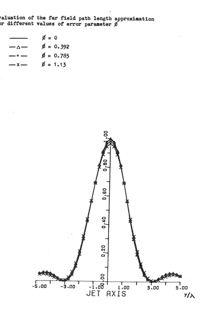
2.3-5. Evaluation of the Far Field Path length Approximation for different values of Error Parameter ^
2.6-8. Source Images of an Off Axis Source
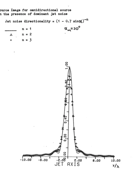
2.9. Source Image for an Omnidirectional Source in the
presence of Dominant Jet Noise
2.10. Source Image of an Omnidirectional Point Source in the
presence of Jet Noise of Equal Signifioanoe.
2.11. Source Image for a l&egian of Jet Noise la the presence of
an Omnidirectional Source of Equal Significance.
Fig.3.1. Basic Principle of the Wavenumber Spectrum.
3.2. The Analogy between the evaluation of a Power Spectral Density Function, and the evaluation of the Source Distribution.
3.3. Example of Reduced Graded Microphone Array
3 . 4 . Amplitude and Phase Data for Continuous Source Distribution 3.5. Transform of Continuous Source Distribution
3 . 6 . Amplitude and Phase Data for Continuous Source Distribution plus Two Point Sources.
3.7. Transform of Continuous Source Distribution with Two Point Sources using linear Interpolation.
3 . 8 . Transform of Continuous Source Distribution with Two Point Sources using a Fourier Series Solution.
3.9 - 1 4 Error Analysis: Comparison of Theory with Practice
3.15 Transmission of Errors to Source Distribution
3 . 1 6 Comparison of Measured Errors with Theory Fig.4.1. Analog Method
4 . 2 . Analog/Digital Method 4.3. Digital Computer Method
4 . 4 . layout of Equipment for Calculation of C.P.S.D. using Narrow-band Cross Correlation
4.5. Layout of Equipment for Calculation of C.P.S.D. using Overall Cross Correlation
4 . 6 . Principle of the Programme Suite on ISVR PDP 11/50 for Polar Correlation
4*7. Block Diagram of Programmes on the Alpha Computer
4.9. Flo* Chart for the Calculation of C.P.8.D. in PAMA
4.10 Calculation of Source Distribution
Fig.5.1. General Arrangement of Horizontal Jet Rig in ISVR Anechoic
Chamber
5.2-10 Source Distributions fi-om a 1 inch Cold Jet
5.11 Measure Time Delays from Loudspeaker Tests
5.12 Time Delay Correction Factors for Polar Arc Centre
Misalignment.
5.1) Speotra for NGTE Testa at 92^ to Jet Axis
5.14-18 Results f^om Noise Test Paoility &t NGTE
Fig.6.1. Scaled Diagrams of Engine
6.2-12 Results from RB.211 Q.E.D.
6.13 Integrated Bartlett Window Function
6.14 Comparison of Measured Levels
6.15 Attenuation of Tailpipe Noise by Bulk Absorber vs Frequency
6.16 Measured Levels of Jet Noise vs Engine Condition
LIST OP SYMBOLS
a Speed of sound
a^(z) Distribution of sources within coherent region at freq.' <0 '
B Effective bandwidth of spectral window
B T Product of B^ with length of signal received
Coherence of signals measured at X and ^ on polar arc
C^ Coherence of signals measured at microphone m and ref mic.
D^(y, (X ) Directionality of coherent region located at 'y'
d(o< ) Directionality of source distribution
1 Error in measured coherence at microphone 'm'
1 Typical value of ^
f Frequency in Hz
(r^(w ) C.P.S.D, at freq. '(J ' between signals x and y
l ( w ) Power spectral level of sources at freq.'o '
K Acoustic wavenumber = Zir/X
L Aliasing length
M, M' General integer variable,
M Convection Mach No.
c
M Mach no. of wind
w
Mqj Resolved Mach of wind
m Integer variable
N General integer variable
Engine speed variable as % of maximum operational fan shaft speed.
NS No. of sauries in data block
o( ) Order function
( % ) Power spectral density at angle ' oc ' on polar arc at freq.<*) .
p(u ,t) Pressure fluctuations at ' oc ' on polar arc
p ^ ( ) Frequency component of pressure fluctuations at ' on polar
arc
Q-p (y) Source strength variable viewed from p
Q(y) Source strength variable
q(y,t) Source fluctuations as function of time at location 'y'
less (y) Frequency component of source fluctuations at 'y'
R Polar arc radius
R_ (oC ) C.P.S.D. at frequency 'w ' between signals at oi and
^ on Polar arc
S Standard deviation
t Time variable (with subscripts)
T Length of time averaging
W( ) Window function
w( ksin ) Weighting funoti on
X Distance variable
y Distance variable
7,(7^,72*^3) Spatial cartesian vectors
Y ( M ) Effective bandwidth of spatial data window
a Distance variable
^ Angle on Polar aire
0( Aperture angle (max value of ^ in array)
Reference angle on Polar arc
A Microphone spacing in(sinec)
X Acoustic wavelength
T T = 3.14159
t Time or time delay variable with subscripts
p Phase variable
UNTVEBSITT OP SOUTHAMPTON
ABSTRACT
FACULTY OP ENGINEERING
INSTITUTE OP SOUND AND VIBRATION aE&BARCH
Dootor of Philosophy
JET NOISE SOURCE LOCATION
by Stewart Glegg
This thesis describes the development of a technique which evaluates
the relative strengths of noise sowroes on jet engines. At the outset
the technique, known as Polar Correlation, had been shown to work in
practice, and the purpose of this project was to refine it into a
method suitable for general application.
In this thesis each aspect of this technique has been covered,
starting with its theoretical background and concluding with its
application to jet engines. Also included in this work is a
discuss-ion of the practical applicatdiscuss-ion of the technique, the development of
data analysis systems, and experimental results on a number of different
rigs.
The Polar Correlation technique samples the wavefield produced by a
linear distribution of acoustic sources. Prom these measurements a
resolution limited source image is obtained by inverting the wavenumber
spectrum of the acoustic source distribution. The theoretical
back-ground to the technique, and the implications of the approximations
which are required, are outlined in Chapter Two. The practical aspects
of the technique and its application are described in Chapter Three. A
major part of the work has been the development of data analysis systems
which provide fast and efficient data reduction. Several different
methods have been used and these are described in Chapter Four. The
application of the technique to hot and cold model air jets, and full
scale jet engines (specifically the Rolls Royce EB.211) are described
in Chapters Five and Six.
In conclusion this technique has been used successfully for the
location of jet noise sources at both full and model scale, and data
analysis facilities for the technique have been established at both ISVR,
— 1 —
CHAPTER 1: INTRODUCTION
1.1. INTRODUCTION
One of the major aspects of controlling the noise output from
a complicated machine such as a jet engine is the evaluation of the
areas to which noise reduction techniques can be most effectively
applied. Only when the relative significance of each noise source
is known can the most effective action be taken to reduce the overall
noise output. While this is a very general problem which is
signif-icant in many applications of noise control, the work described in
this thesis is limited to the evaluation of the noise sources on
aero-engines. On a m o d e m aero-engine there are several different sources
of noise and several channels through which this noise may escape
to the acoustic far field. For instance engine fan noise is
trans-mitted either upstream and out of the engine inlet, or downstream
and out of the by-pass duct exit, while combustion noise is emitted
mainly by the hot core exhaust (see Figure 1.1). As well as these
sources there also exists jet noise caused by the turbulent mixing
of the jet exhaust with the outside medium. Determination of the
relative levels of these sources permits the development engineer to
concentrate acoustic treatment on those sources where the greatest
net benefit is anticipated.
The simplest and most widely used technique of estimating the
strengths of acoustic sources on jet engines is prediction and spectral
analysis. If the spectral characteristics of each type of source can
be predicted, then the measured frequency spectrum will show the level
of each source. However this technique is limited to sources with
known spectral characteristics, and it is only possible to
different-iate between sources which do not contribute equally at a particular
frequency. Although these methods have been used for many years in
the aircraft industry, they are not very satisfactory because too much
has to be assumed about the acoustic sources. Therefore there is a
requirement for techniques which measure the relative strength of each
source within a distribution at a specified frequency, without the
necessity for the source characteristics to be known in advance. This
thesis will describe a technique, known as Polar Correlation, which
may be used to evaluate the relative strengths of sources along the
—2—
1.2. THE POLAR CQRRaLAIIQN TECHNIQUE
Before reviewing the many different methods whioh have been used
to evaluate eeuroea of noise, the principle of Polar Correlation will
be introduced. The noise eeuroe* on a jet engine emit acoustic waves
which propagate into the acoustic far field, and the fluctuations at
any point in this field are determined by the strength and
distrib-ution of acoustic sources on the engine. For example consider three
simple harmonically fluctuating sources on a line as illustrated in
Figure 3*1. The wavefleld at a fixed instant in time for each source
in isolation is illustrated on the left of this figure, and the overall
wavefield is given by the sum of these three. The principle of source
location on which Polar Correlation is based can be demonstrated by
considering this simple model. Polar Correlation evaluates the source
strength distribution by taking measurements on a polar arc of constant
radius in the acoustic far field (see Figure 3.1). First consider
the source at A in isolation: since this lies at the centre of the
polar are, at any fixed Instant of time the fluctuating pressure on
the polar arc will be constant, as illustrated by the top diagram on
the right of Figure 3.1 • However the waves from the source at B cross
over the polar arc, and so at any fixed instant in time there will be
a variation of pressure around the polar arc. This variation is
shown on the right of Figure 3.1 and is found to be cosiatisoidal as a
function of the sine of the angle 'o(*. Similarly for the source at
C which lies further downstream from the polar arc centre. In this
case the polar arc passes through more peaks and troughs of the
wave-field and the variation of pressure as a function of sin( (si ) yields a
cosine wave of higher frequency.
When all three sources are radiating at the same time the total
wavefield on the polar arc will be given by the sum of these three
cosine waves, illustrated on the bottom right of Figure 3.1. However
each cosine wave represents a term in the Fourier series which
repres-ents the total wavefield. The amplitude of each cosine wave 1*
determined by the strength of the source, and the frequency by the
location of the source. It is a relatively simple matter to solve
this Fourier series to determine the strength and location of each
source. In the more general case, sources are continuously
diatrib-uted along the axis of an aero-engine, and therefore the Fourier series
-3-However in the ease of aero-sngines the acoustio sources are
also randomly fluctuating, which means that the effective source
strength at any frequency will vary with time. Therefore it is
necessary to consider an averaged source strength. This may be
obtained by considering the cross power spectral density* on the
polar arc. This quantity is chosen because it retains the important
phase relationships of the randomly fluctuating field which are
required to evaluate the source distribution. It will be shown in
Chapter 2 that there is a Fourier integral relationship between the
distribution of source strength and the cross power spectral density
in the acoustic far field. Thi* integral relationship may be
inverted numerically to yield a resolution limited image of the
acoustic source distribution.
It should be noted that in principle only an "apparent" image
of the source distribution can be obtained. The word "apparent" is
used in this context because there are many different source
distrib-utions which can create the same acoustic far field. Therefore
there are many different reconstructions which can be obtained from
the same set of far field measurements, and the results which are
obtained depend on the assumptions made about the source distribution.
These assumptions constitute the model of the source distribution and
the value of the reconstructed image depends on the accuracy of this
model. This point will be considered in more detail in Chapter 2,
and the rest of this chapter will describe some of the other methods
of source location which have been used.
1.3. LirmAIOEZ EEVIB*
1.3.1. Sonar
The first engineering application of measuring acoustic waves
to determine their source originated in the Great War with the
develop-ment of sonar. This technique was developed by Solokov and its
principle application is the detection of submarines. Like Polar
Correlation, sonar techniques use an array of transducers to evaluate
an acoustic wavefield. From these measurements the angle of arrival
of the acoustic wave is estimated, and this yields the bearing of its
-4-souro® to the array; by using two arrays, two bearings are obtained
and this enables the position of the source to be evaluated. Sonars
can be either active or passive, the former relying on reflections
of a reference acoustic signal, while the latter relies solely on the
noise emitted by the target. There is a large amount of literature
assoc-iated with sonar,and very sophlstioated teohnigues have been developed
to enhance resolution (e.g. Davids, Thurston and Mueeer (1952), van
Buren (1973)), and to reduce signal to noise ratios (Brown and Eeynoulds
(1959)). Although Polar Correlation and sonar have a great deal in
common, their application is very different. In Polar Correlation it
is the relative strengths of sources at approximately known locations
which are required,while with sonar it is the detection of a single
source in a noisy environment which is evaluated. Therefore in
developing Polar Correlation to date, little use has been made of the
more sophisticated techniques used in sonar analysis. However, there
may be some aspects of sonar technology which can be used in the future
to optimise the Polar Correlation technique.
Another method of source identification which has been developed
is acoustic holography. This is a method of measuring the acoustic
wavefield on a plane so that it may be reconstructed either optically
or numerically to give an image of the sources contributing to the
hologram.
In its active application holography is used to obtain the
image of reflecting objects, which are illuminated using sound waves.
However, in order to overcome resolution problems the size of the
illuminated objects must be very much larger than the acoustic
wave-length of the reflected sound. Therefore in most examples of this
technique ultrasonic waves have been used (Mueller (1971), Aoki (1970),
El-8um (1969))
Passive holography has also been used in a number of
applicat-ions. For instance a comprehensive study of vibrating plates using
holographic methods was undertaken by Watson (1975). In his study
Watson measured a microphone signal on a plane in the acoustic far
field of the vibrating plate; this was then added to the signal used
to drive the plate and the combination illuminated an intensity
-5-the microphone over -5-the hologram plane and photographing -5-the diode
light, an optical hologram was produced. Illuminating the hologram
with laser light then gave the image of the field from the vibrating
plate. Similar results have been reported by Greene (1969), who
recorded the distribution of hologram intensity directly without
recourse to optical processing.
Passive holography used to determine the location of a single
source producing G a u ^ a n noise is reported by MacDonald and Shulthesis
(1968), and Hahn (1975). Also Uhea et al (1975) have reported using
holography to identify the source of gear noise. However holography
is very sensitive to signal/noise errors and so Sasaki et al (1977)
have developed a more sophisticated method of signal processing using
polyspectra. Numerical examples show this provides improved images
but this method can only be applied to quasi-periodic sources.
From this review of holographic techniques it would appear that
some of the major problems with source location on jet engines have
not been attempted. First there is the practical problem of applying
a holographic technique to a full scale jet engine on an open air test
bed, and secondly the application of this method to source
distribut-ion with partial spatial coherence has not been investigated. These
problems may result in limitations of the holographic technique, irtdch
could prove difficult to overcome.
i.3'3- Measurement of Jet Noise Source Distributions
One of the environmental noise problems of the last twenty
years has been the effect of jet aircraft noise on the community close
to airports, and this has resulted in a considerable amount of research
into all aspects of jet engine noise. The mechanism which causes jet
noise was originally explained by Lighthill (1952) in terms of the
turbulent mixing process between the jet and the medium into which it
exhausts. However to improve the understanding of jet noise it is
useful to have some knowledge of the distribution of noise source
intensity in the jet, and it is this objective which has inspired a
number of investigations into the acoustic source distributions along
model air jets.
Some of the earlier attempts to measure source distributions
in jets have concentrated on evaluating various properties of the
_6_
considerations (see for example Dyer (1959), Maestrello & McDavid
(1971)). However more recently a number of techniques have been
developed which measure directly the distribution of source strength
along both model and full scale jets, and in this section each of
these methods will be reviewed.
a) Shield*
The first attempts to measure the distribution of acoustic
source strength within a jet from acoustic far field measurements
alone utilised shields to eliminate part of the sowrce distribution
(Potter & Jones (19^7), Bishop et al (1971))• The principle of this
method relies on"what cannot be seen cannot be heard",which considering
the discrepancy in wavelengths between optics and acoustics is perhaps
an oversimplification. More recently, Damns (1977) has developed a
theoretical interpretation of this type of measurement, and this has
been applied to some data from the RB.211 engine (Beasley (1977))•
The problem with this method is that the jet engine has to be modelled
not only as a line source but also as a number of individual sources.
The advantages of this technique are that first,the individual sources
can be placed at locations where point sources are known to exist,
thus theoretically giving infinite resolution and secondly,the
direct-ionality of each of these modelled sources can be evaluated. However
there are also some major disadvantages: first, as the number of
modelled sources are increased, the method used to calculate the source
levels becomes numerically unstable and secondly, there is a major
exp-erimental problem in applying this method to a full scale jet engine.
On the RB.211 a screen 28m long and ICte high was used in 26 different
locations. This programme took several days to complete and required
a number of engine runs. Compared with the microphone array
tech-niques which have been used to obtain similar information on a single
engine run, the shield technique would appear to have major practical
disadvantages.
b) Causality Correlation
An ingenious technique of source location, known as Causality
Correlation, has recently been developed by Bidden (1973). This
technique has primarily been developed to measure jet noise sources
although in principle it may also be used on other source mechanisms.
-7-of an acouatio source to the far field intensity depends not only on
the fluctuations of that source but also on its interference effects
with other sources. Therefore to predict the acoustic far field
from source measurements alone requires the evaluation of not only
each source amplitude but also its cross-correlation with every other
source. Attempts to measure this complete description of the sources
in model air jets have never been successful because of the enormous
measurement programme required and the fundamental difficulties of
measuring the source strength. Therefore Siddon has proposed a
method of source strength measurement which automatically includes
the interference between each source.
The principle of Siddons technique is to cross-correlate source
fluctuations with the acoustic far field signal. Since the far
field signal includes contributions from all the sources within the
distribution, all interference effects are automatically Included, and
the resultant correlation at the appropriate time delay specifies the
effective radiated intensity of the source fluctuations being measured.
The advantage of this method is that it offers a direct link
between a local region of the source and a specific far field observer,
thus avoiding the resolution problem associated with the other far
field methods. However,it should be noted that when considering the
complete source distribution, probe measurements must be taken at
intervals which are small compared with the acoustic wavelengths In
order to account for interference effects, and to ensure integral
closure (i.e. the integrated source intensity gives the far field
level). There are also a number of quite severe practical problems
which may offset the advantage of ideal resolution, in
particular:-i) Although the method offers at least an order of magnitude saving
in experimental effort compared with source measurement alone, the
level of effort required is still very appreciable and leads to a
degree of detail beyond that required in all but the most fundamental
research applications,
11) Application of this technique requires a quite detailed knowledge
of the noise producing mechanisms involved,since this determines the
8
-iii) The employment of a probe in the source region raises the problem
of probe generated noise. The criterion for probe noise is
partic-ularly severe for causality correlation (see Siddon (1973)), since
it must be negligible compared to that generated by the locally
corr-elated source region in which the probe is located. This is a severe
restriction and more seriously, there is no obvious experimental method
of ensuring that it is obeyed. The probe noise could frequently be
negligible compared to that produced by the total source region, while
still being the dominant contributor in the locally correlated region
in which it is placed. It is noted however that remote sensing
devices, for example the Laser Doppler Velocimeter for velocity
measure-ments, could eliminate this particular problem eurea.
iv) Finally it should be noted that the amplitude of the correlations
to be measured will frequently be small, the average correlation
coefficient being of the order of the reciprocal of the squatre root
of the number of locally correlated regions contained in the total
source array. Dauams (1977) has also pointed out that they could also
be appreciably smaller than this if a significant part of the 'source'
signal is composed of the convection of a frozen pattern of
fluctuat-ions past the probe, as these will not contribute to the far field
pressure.
In conclusion, it would appear that these difficulties make
Causality Correlation unsuitable as a general purpose source location
technique. Its application is probably restricted to specific
research problems, but even here considerable care in its practical
implementation is required if erroneous or misleading information is
to be avoided.
c) Acoustic Mirrors
The first attempts to use the focusing properties of concave
surfaces for source location in the context of aerodynamic noise appear
to be those of Grosohe (1968) and Chu et al (1972) (see also Grosche
(1973)). The former used an elliptical mirror while the latter a
parabolic one. The parabolic mirror focuses all rays arriving
parallel to the mirror axis onto a microphone plaoed at the focal
point. This is strictly only appropriate for a source at infinity,
but it has been shown by Glegg (1975) that in practice this is not a
-9-mirror can only locate the line (i.e. the -9-mirror axis) on which the
source must lie, and does not have resolution along this axis.
However,the elliptical mirror focuses radiation from a source placed
at one focal point to a microphone placed at the other. It therefore
provides three dimensional focusing which can be an advantagei
The characteristic of acoustic mirrors which permits their use
as source location devices is that the path length from the source at
one focus to the microphone at the other, via the mirror surface, are
equal. Thus if the amplitude and phase of wave emitted by the source
is constant on the surface of a sphere centred on the source, all the
rays will arrive at the microphone in phase and interfere
construct-ively to yield a large signal. Alternatively,if the source does not
lie on the focus, the rays reaching the microphone will have different
path lengths and will interfere destructively, resulting in a smaller
microphone signal.
However, the requirement for omnidirectional amplitude and phase
restricts such techniques to evaluating the effective monopole source
strength. It should be emphasised that this is a common feature of
all far field source location techniques and is an example of the
inherent non-uniqueness of the relationship between the acoustic far
field and the source distribution (Ffowcs-Williams (1973), Kempton
(1976)). However, the image of a source with directional
character-istics similar to jet noise has been investigated by G-legg (1975) and
it was shown that the effect of the directionality was not severe,
merely degrading the resolution of the mirror.
While acoustic mirrors have been very successful as source
location tools at model scale, there is a major practical problem in
applying the same technique to full scale engines where the wavelengths
of interest are very much longer. It may be shown that to obtain
resolution of about 5 acoustic wavelengths, the mirror diameter must
be about 50-73& of the customary far field measurement distance. On
a full scale engine this could result in mirrors which are at least
10 m in diameter, and an accurate scanning mechanism for this mirror
would obviously introduce major mechanical problems on an open air
test site. Consequently acoustic mirrors have never been developed
—i 0""
d) Mierophone Arrays
Perhaps the major practical problem of using acoustic mirrors
for source location on jets is their lack of applicability to different
test rigs. A mirror is a large and expensive apparatus and has to be
optimised for a particular application. Consequently there are major
practical problems in designing and building a mirror which may be
used on a number of test rigs at both model and full scale. As a
result,microphone array techniques have been developed which provide
equal ability to resolve sources as the mirror, and may be applied to
many different rigs. In principle a microphone array technique is
merely a simplification of the mirror. Rather than sample a segment
of the wavefield and acoustically construct a source image, the
micro-phone array samples the wavefield at specific points, and constructs
the source image using signal processing techniques.
In the last five years a number of microphone array techniques
have been developed specifically for the evaluation of jet noise
sources. It would appear that the most widely applied of these
tech-niques are the Acoustic Telescope (Billingsley and Kinns (1976)) and
Polar Correlation (Fisher et al (1977)), while other techniques due
to Parthasarathy (1974), Kinns (1976) and Maestrello and Liu (1976)
have also been reported with a limited set of experimental results.
The Acoustic Telescope and Polar Correlation were developed
con-currently at Cambridge University by Billingsley and Kinns, and at
Southampton University by Harper-Bourne respectively, both under the
sponsorship of Rolls Royce (1971) Ltd. Although these two techniques
work on different principles, it has transpired that there is very
little difference between the results which can be obtained using
either technique. A detailed comparison by Damms (1977) concludes
that theoretically there is no difference between these methods, and
so the only advantages of one method over the other must result from
practical considerations. In this respect each technique has its own
advantages, which depend on the particular requirement of each test.
The advantage of the Acoustic Telescope is its very fast data analysis
which enables source distributions to be computed in real time; however
it can only be applied using a specially developed mini-computer and
it does not provide any intermediate storage medium between the
1 1
-Polar Correlation requires a longer data analysis procedure but has
the advantages of providing an intermediate data storage medium, and
requiring less sophisticated data analysis systems.
The source location method used in the Acoustic Telescope relies
on the same principle as sonar techniques. The Telescope consists
of a linear array of equally spaced microphones in the acoustic far
field; and may be focused onto a source in the distribution. The
focusing is achieved by linearly summing the signals from each
micro-phone in the array at the time delay appropriate to the acoustic
propagation time from the source to each microphone. Therefore
focusing is achieved in the same way as the acoustic mirror. The
Polar Correlation technique however samples the signals in the acoustic
far field in a similar way using microphones on a polar aire and
utilises the relationship between amplitude and phase of these signals
at specific frequencies to construct a wavenumber spectrum of the
source distribution. Inverting the wavenumber spectrum provides an
image of the source distribution. Since both techniques sample the
wavefield using similar methods, a number of the principles developed
in this thesis on wavefield sampling are equally applicable to both
techniques.
In order to compare these two methods with other microphone
array techniques the principle of each will be described and their
limitations discussed.
i) Parthasarathys' Method; In this technique the signals Arom two
microphones in the acoustic far field are cross correlated. Then by
assuming that each source in the distribution is uncorrelated and
produces pure white noise, the evaluated cross correlation gives the
distribution of source strength intensity along the jet. The fallacy
of this method lies in the assumptions made about the noise sources. Jet
noise sources do not necessarily produce purely random white noise
signals, and the source spectrum may vary along the aais of the jet.
In principle this method is limited by these assumptions to very
specific applications and the results presented (Parthasarathy (1974))
do not provide particularly well resolved source distributions.
ii) Binaural Source Location; This method was developed by Kinns
(1976) and evaluates the centroid of a source distribution from the
1 2
-far field. In common with other source location techniques this
method assumes that the jet noise sources lie on the centre line of
the jet, and in principle this method is the aero aperture limit of
Polar Correlation. While this method locates the source centroid
exactly (within the limitations of its source strength definition) it
provides no resolution and therefore gives no information about the
distribution of sources. Consequently it is of only limited
applic-ation.
iii) Maestrellos' Method; This technique developed by Maestrello
and Liu (1976) uses a microphone array similar to that of Polar
Correlation, with microphones equally spaced on a polar arc in the
acoustic far field. By cross correlating the signals between each
microphone it is shown that there is a double wavenumber integral
relationship between the measurements and the cross spectral density
between sources in the distribution. This relationship will be
demon-strated in the development of the theory pertaining to Polar
Correl-ation in Chapter 2, and it is at this stage that the two methods
diverge. In Polar Correlation the source strength is defined so
that interference effects between sources are included in a single
source strength definition, which reduces the relationship with the
measurements frcm a double to a single wavenumber integral which may
be inverted. In Maestrellos' method the double integral is solved
using a curve fitting procedure. There are two criticisms of
Maestrellos' work: first his analysis does not admit the existence
of phase relationships between coherent sources, and this automatically
excludes any convected source model of jet noise. Secondly,no
analysis of measurement error sensitivity has been undertaken and
according to Yardley (1974) this is likely to cause uncharacteristic
errors in the numerical inversion procedures used to obtain source
distributions.
1.3.4. Conclusion
In this section an attempt has been made to review all the
relevant methods of acoustic source location. Specifically we are
interested in methods which can be applied to the evaluation of sources
on jet engines. Although there are many methods which have been
applied to model scale jets, there are only two which have been used
- 1 ^
these are the Acoustic Telescope and Polar Correlation. It has been
shown that although these two teohniques use different methods of
analysis, they are capable of produoing the same results and are
subject to the same limitations. The choice of technique therefore
depends on the requirements of a particular test.
In the following chapters, development work on the Polar
Correl-ation technique will be described. However due to its close
relation-ship with the Acoustic Telescope a number of the principles developed
are equally relevant to both tehcniques, particularly those relating
to the sampling of waveflelds. It is hoped that this work will go
some way to justify the claim that Polar Correlation is at present one
of the two more sophisticated techniques for evaluating the
.14-CHAPTER 2; THE THEORY OP SOURCE LOCATION TECHNIQUES WITH PARTICULAR REFERENCE TO POLAR CORRELATION
2.1. INTRODUCTION
This chapter describes in detail the theoretical background to the
Polar Correlation technique. However since this technique has a great
deal in common with other source location techniques used to evaluate
the source distributions on jet engines, a number of the theorems
devel-oped have a far more general application.
The basic restriction of source location methods which use one
dimensional microphone arrays, such as Polar Correlation or the Acoustic
Telescope (Billingsley & Kinns (1976)), is that the source distribution
must be modelled as an effective line source. Therefore the starting
point of this chapter is the solution to the wave equation which
des-cribes the acoustic field from such a distribution of sources. Prom
this the principle of the wave number spectrum and its extension to
Polar Correlation is developed.
One of the purposes of this chapter is to evaluate the
signific-ance of the assumptions and restrictions which are implicit in the
application of Polar Correlation. These are discussed in terms of the
evaluated source image, and the effects of axial resolution, aliasing
lengths, and three dimensional effects are demonstrated. These effects
are not solely a feature of Polar Correlation but are equally important
in other methods of source location.
One of the inherent problems with any method of source location
which uses measurements in the acoustic far field is the non-uniqueness
of the results. This ambiguity arises because there are many different
distributions of sources which cause the same acoustic far field;
however from the far field information alone any source location
tech-nique can only define one apparent source distribution. This can be
defined as the equivalent monopole source distribution, which may, in
principle, be replaced by many other distributions of higher order
multipole sources. At first sight this ambiguity might be considered
so catastrophic that all far field source location techniques are
rend-ered useless. However in practice the acoustic far field information
is rarely the only information available. When undertaking an
-15-soTjrce is known, and the information required, is the relative level of
each source within the distribution. To a certain extent this
over-comes the ambiguity of the results since they may be checked against
this additional information.
One of the problem areas of practical source location techniques
is their application to randomly fluctuating sources with arbitary
spatial coherence. This aspect is discussed in some detail and two
different definitions of source level are developed. The first
defin-ition gives the effective source strength as seen by an observer at a
reference position, and the second defines the relative strength of each
region of coherent sources. The latter definition requires that each
coherent structure is the same throughout the source distribution, and
is therefore of limited application, whereas the former definition is
more general but is also more difficult to both measure and interpret.
Finally it should be noted that this chapter is entirely of a
theoretical nature and no attempt has been made to describe theorems in
terms of their practical application. Therefore any reader who is
only interested in applying this technique should immediately turn to
Chapter Three, where the principles and application of this technique
will be described without so much mathematical analysis.
2.2. THE WAVENUMBER SPECTRUM PRINCIPLE
The acoustic signal from a linear array of sources of strength
q(y,t) may be defined by the integral
OO
= J q(y,t - r/a^) dy/r (2.2.l)
- oA
This is the well known solution to the wave equation in an acoustic
field free from reflections; the pressure p( o( ,t) may be taken on a
polar arc of constant radius R (see Figure 2,1) and the distance 'r' is
defined as the propagation path length between the source at 'y' and
the measurement point.
By taking the Fourier transform of both sides of this equation,
a complex valued acoustic field strength is defined at the fixed
frequency 'ca': eO
= J S u / y ) 3y/r (2.2.2)
-cA
- 1 6 —
At this stage it is convenient to note that in the acoustic far
field, where the polar arc radius R is very much greater than the
length of the source distribution L, the propagation path length can
be approximated by r = R - ysintA. + o(y ); this is a fundamental
approximation to all that follows and & e effect of ignoring higher
order terms in this series will be demonstrated later in this chapter.
Further, in the amplitude term of 1/r, the dependence on 'y' may
be dropped altogether without any significant loss of accuracy, and
the complex aoouatio field ia defined as
) = 5 Cy) dy (2.2.3)
This equation shows a Fourier transform relationship between the
distribution of source strength and the complex pressure amplitude on
the polar arc, and the quantity ^ (of ) is knomi as the wavenumber
spectrum of the source distribution g ^ ( y ) . This suggests that by
taking the inverse Fourier transform of ^ (oL ) as a function of
'KsinoL'*, it is possible to evaluate the distribution of source
strength q ^ ( y ) .
2.3. PHYSICAL PROBLEMS OF.WAVEMUMBER SPECTRA
It has been shown in the previous section that in principle the
wavenumber spectrum may be used to evaluate the source distribution
from measurements in the acoustic far field. However in practice there
are several physical limitations which prevent an exact solution being
obtained. These problems restrict the solution of the wavenumber
spectrum so that at best only an apparent source image may be evaluated.
This section will discuss the physical restrictions which are imposed,
and their effect on the apparent source image.
a) Resolution
In order to evaluate the inverse Fourier transform of a function
such as the complex acoustic field, p ^ [ d ), it is necessary to measure
this function between the infinite limits -oo/^Ksinw/ao . However
this is physically impossible since measurements can only be made
between the finite limits -Ksind < Ksinat/Ksin where sin x 1 . In
m \ m A m ^
order to investigate the significance of this restriction, it is
-17-ient to multiply the acoustic field measurements by an arbitary
weighting function which is zero outside the limits of the measurements.
The infinite limits to the integral may then be used and the
measure-ment restrictions are defined by the effects of the weighting function
on the source image.
The measurable source image, 'q'jCy), can therefore be calculated
from the inverse Fourier transform of the acoustic field, ^ ),
mult-iplied by an arbitary weighting function w(EsinQ() which is zero outside
the measurement limits of - Esino( : m
oO
*(K8in»() (2.3.1)
where w(Ksinot) = 0 when | Ksinotj ^ Ksin X,
A property of Fourier transforms is that the inverse transform of
the product of two functions yields a convolution integral of the type
(Churchill (1972), p.393)
uut e
^ ( z ) = 2 j (y) w(y-z) dy (2.3.2)
-00
where W(y) is the inverse Fourier transform of the weighting function
w(K8inQ() and % (y) exp(iZR)/R is the inverse transform of the acoustic
field (o( ), as defined by equation 2.2.3.
This shows that the effect of the limited range of measurements
and the choice of weighting function is to smooth the finer detail of
the source image. Since the choice of weighting function is arbitary,
the amount of smoothing on the source image can be controlled to a
certain extent. For instance two typical weightings which may be used
are the rectangular weighting and the Bartlett (triangular) weighting
defined by:
Rectangular: w(Ksinoi ) = 1.0 iKsincCl ^ E s i n ^ ^ (2.3.3)
= 0.0 1 KsinKi ^ Ksinof^
Bartlett: w(Ksino< ) = 1- 1 KsinX 1 |Ksin«(| ^ Ksin K
E s i n x ^
= 0.0 (Ksino<( ^ EsinCK^
The source images of a simple point source using these weightings
are shown in Figure 2.2, and the width of the main lobe in these images
1 8
-In order to demonstrate the dependence of the window function
W(y) on the aperture angle ' and the wavenumber 'K', it is
convenient to specify W(y) and the weighting function w(x.) as Fourier
transform pairs: i.e.
W(y) = ^ J *(E8ln*) (2.3.4)
~<ia
To eliminate the effect of the aperture angle it is useful to note that
all weightings are functions of KsinoC/Ksln = x , and so 2.3.4 may
also be written as
W(y) = glp w(x ) dx (2.3.5)
—oO
where we have substituted x = Kain^C/XsinoC
Then by defining a normalised window function W which is
indepen-dent of wavenumber 'K' and aperture angle ' and related to the
weighting function by the Fourier Transform %o
%m(y) = (*)
it follows from 2.3.5 that
W(y) = Esinc*^ . WQCKysinotQ^ (2.3.6)
This result, which shows that the window function depends upon
Kysinol , demonstrates that the resolution, or width of the main lobe,
will be inversely proportional to KslnoC . Also the peak level of the
window will be proportional to KsinOl while the area beneath the curve
remains independent of EsinOC . Therefore good resolution is obtained
using large aperture angles 'o<. ' and high frequencies so that 'Esin K ^
is large.
The weighting/window functions discussed above are identical to
the weighting/window functions used in spectral analysis (Blackman and
Tukey (1958)). There are many different types of these functions,
and in general these have either large side lobes (e.g. the rectangular
window in Figure 2.2) with a narrow main lobe or smaller side lobes
(e.g. the Bartlett window Figure 2.2) with a broader main lobe. In
this application the main requirement is for the best resolution without
1 9
-standard window functions, the Bartlett most closely satisfied these
criteria. Therefore the Bartlett window has been used as standard in
all the source images presented in this thesis.
In order to evaluate the source image as defined by equation
2,3.1, it is necessary to measure the function ((X.) as a continuous
function of the wavenumber space variable 'Ksin&C'. In practice
however it is only possible to evaluate p ^ (ol) at a finite number of
points in space. This effectively imposes a further physical
restric-tion on the source image which may be defined as the aliasing problem.
This problem applies not only to Polar Correlation, but to any scheme
idiich usee discrete measurements in the acoustic far field.
In order to demonstrate this problem consider a measurement array
which evaluates the field at equal locations^ in 'sin#('. The complex
field at the nth location is given by
5 (1) = e ™ r 5 (y) e - ^ ^ a y
w R ^ ^
Alternatively this equation may be written as
^ ( n ) = e ^ exp(iELnA) f
O n V W
By choosing KlmAi = 2Trn, the term ezp(iZLnA) is unity, and it
follows that the measurements p ^ ( n ) cannot differentiate between the
source distributions q ^ ( y ) , q^^ (y-L) q^(ytml). Therefore the
source image calculated from the measurements p^j (n) must be periodic
with period 'L', and errors will occur if the source distribution is
significant outside the limits y = - L/2, where L is defined by the
spacing L = X / ^ (since K = 2tr/\ .)
c) Three Dimensional Effects
The model considered in Section 2.2 consisted of a linear array
of sources on the y-axis. However in practice the type of source
distributions to be considered are those from aero engines which have
finite dimensions perpendicular to the y axis. Therefore it is
necessary to consider the conditions under which the three dimensional
source distribution may be considered.
Starting with the solution to the wave equation in three
2 0
-p(oi ,t) = j j j q'(y, t-r/a ) dy, d y V r (2.3.?)
By taking the Fourier transform with respect to time of this equation
we obtain:
= jTjjT q' (y) dy^ dy^ dy /r (2.3.8)
In the three dimensional oase the far field approzimation for the path
length 'r' is given Dy
. t .
r = R - y^sinK-ygCosK* O&j/rJ
and in the amplitude term 1/r, the y^, y^ dependence in this
approxim-ation may be ignored without significant loss of accuracy. Therefore
equation 2.3.8 may be written:
I I J (y) (2.3.9)
a 7172^3
%hen the yg dimension is small such that K y g ^ K l , then expf-iEygCOsPC) =1
and an equivalent linear source strength may be defined as
q%(yi) = j\f %%(?) Sfg (2.3.10)
A/
- '3
^2^3
such that
I q „ ( y i ) (2.3.11)
R
which is equivalent to equation 2.2.3.
This demonstrates how the source distribution may be considered
as a line source providing the dimensions in the y^ direction are very
much less than a wavelength so that Eyg .
This condition may be relaxed slightly if the wavenumber spectrum
is only evaluated over the limited range of - EsinoC . In this case
it is necessary that KygCl-cos ^ ^ ) ^< 1 so that the integral
I I q ' ( y )
^2^3
is independent of oC over the range - The effective linear
—21 —
( y ^ ) = j v T q ' ( y ) dy_ ( 2 . 3 . 1 2 )
ygy^ <*
which is identical to 2.3.10 when Kjg 1.
While this gives the condition under which the cross axis
dimen-sions may be ignored, the effect of working outside these limitations
will be discussed In a later section.
2.4. AMBIGUOUS SOURCE DISTRIBUTIONS
The relationships derived in the previous sections assume that
the acoustic field may be described in terms of the solution to the
wave equation: ae
p(9(,t) = q(y,t - i/a^) dy/r
However it has been emphasised by Pfowcs Williams (1973), (1974)
that this solution is not unique, and there are many source
distribut-ions q(y,t) which give the same acoustic field. This has been very
concisely demonstrated by Kempton (1976) who has illustrated the
eguiv-alence of acoustic fields from a monopole source at 'y' and a multipole
cluster at the origin 'y=0'. This follows from a Taylors series
expansion of the acoustic field from the monopole of strength A(t):
(see Kempton (1976))
l A { t - r / a „ ) = £ f 5 M t - E / a j ] (2.4.1)
n=o t a n [ R
This series converges whenever R ^ l R - rj. In the acoustic far
2
field terms of order 1/R may be ignored in the derivatives and in the
expansion R-r = ysino< + 0(y^/R). Therefore
r Att-r/a^) = ^ ^ (-y8in*(/&o) ^ A(t-E/ag) (2.4.2)
n=o
Each term in this series is characteristic of a multipole of
order 2^ and strength
[ ( - y / a q ) V n : j A(t) (2.4.3)
I J &tn
located at the origin y = 0. It should be noted however that the far
field approximations leading to 2.4.2 are not strictly necessary since
2 2
-This demonstrates how the same acoustic field has been generated
by two distinctly different mechanisms, and it is therefore very
important that this ambiguity should be considered when interpreting
the results from far field source location techniques.
To investigate this further consider the source image calculated
from the field of a multipole of order 2 , whose strength is given by
2.4.3, using equation 2.3.1. First it is necessary to take the Fourier
transform of 2,4.3 with respect to time, so that the acoustic field at
the fixed frequency ' w ' is defined as
= ( - I K y s i n x ) " A /n! . je^^*
a
where is the Fourier transform of A(t). Then the source image is
given as
-(z) = J* (-xKysinoC ^ - g * (E8inP<.)e^^^^^d(E8inX )
which may be evaluated using the properties of Fourier transforms
(Churchill (1972) p.471,(3)) to give
. iER \ n
q ( z ) = " V .. C - y ) ^ W ( z ) ( 2 . 4 . 4 )
^n
Therefore the source image from a multipole of order 2^ is the nth
derivative of the window function W(z); also note how this is a very
complete result since the source image from a cluster of multipoles
of ascending order, whose strength is given by 2.4.3, is defined as
The series in this equation sums to the window function W(z-y),
and the source image represents a monopole located at 'y', from which
the source strengths 2.4.3 were derived. Therefore the source image
reveals the monopole nature of the source distribution, but conceals
its true nature which may consist of a number of interfering higher
order sources.
2.5. THE EXTEIiSION TO NOISE" SOURCE DISTEIBUTIOffS WITH ^ I T A R Y
SPATIAL COHERENCE
The discussion so far has been limited to sources whose fluctuations
are known for all time, and therefore have exact representations in the
-23-location techniques to randomly fluctuating sources, whose Fourier transform
with respect to time can only be estimated from a limited record. This
estim-ate has to be used because the source strength in the frequency dcmain, and
thus the far field pressure )» will depend not only on frequency
but also on the time of evaluation. Therefore to obtain a meaningful
result it is necessary to consider an averaged quazitity with non-zero
mean. In order to preserve the phase dependence in the far field it
is found that the natural quantity to consider is the cross power
spectral* density, defined as the averaged cross product between
at two points in the acouatic far field.
As before the acoustic far field from an almost linear array of
sources will be considered on a polar arc of radius 'R' (see figure 2.1).
The cross power spectral density will be taken between a reference point
on this arc, defined to be at the angle as shown in Figure 2.1,
and a second point at an angle 'eC '• The cross power spectral density
is defined as the averaged value of the cross product of the acoustic
field variables at these points.
= Ex ) p j / f p / ] (2.5.1)
The location ' is defined as the reference point, at which the
phase will be zero. This may be taken as aqy point on the polar arc.
Therefore evaluating the cross power spectral density ( DC) in terms
of the source strengths given in 2.2.3, the following relationship is
obtained:
V (
=
52 f /
Ex
(y)
Pdya.
r
a y g
L 4
"
^
( 2 . 5 . 2 )
Then by defining the average source level as seen at ' ^ ' by the integral
over z of the cross power spectral density of the source strengths,
E x ^ q ^ ( y ) q ^ (2^including the associated phase lag to ' ^ , i.e.
(y) = 5 2 J Ex (y) az (2.5.3)
it is found that
E p ( » t ) = 1 « p ( y ) -sinp )ay (2.5.4)