James Nelson∗ and Stefano Sanvito†
School of Physics, AMBER and CRANN Institute, Trinity College, Dublin 2, Ireland (Dated: June 21, 2019)
The magnetic properties of a material are determined by a subtle balance between the various interactions at play, a fact that makes the design of new magnets a daunting task. High-throughput electronic structure theory may help to explore the vast chemical space available and offers a design tool to the experimental synthesis. This method efficiently predicts the elementary magnetic prop-erties of a compound and its thermodynamical stability, but it is blind to information concerning the magnetic critical temperature. Here we introduce a range of machine-learning models to predict the Curie temperature, TC, of ferromagnets. The models are constructed by using experimental data for about 2,500 known magnets and consider the chemical composition of a compound as the only feature determiningTC. Thus, we are able to establish a one-to-one relation between the chemical composition and the critical temperature. We show that the best model can predictTC’s with an accuracy of about 50 K. Most importantly our model is able to extrapolate the predictions to regions of the chemical space, where only a little fraction of the data was considered for training. This is demonstrated by tracing theTCof binary intermetallic alloys along their composition space and for the Al-Co-Fe ternary system.
I. INTRODUCTION
Magnets [1, 2], compounds in which the atomic spins arrange themselves yielding a macroscopic order, are known since antiquity, but still represent a fascinating class of materials. In these, the interplay between the local Hund’s coupling, the exchange interaction and the magneto-crystalline anisotropy, is able to generate a mul-titude of ground states, which may differ both at the microscopic and macroscopic level. Often the particular magnetic configuration of a material is the result of a sub-tle balance between the interactions at play, so that the prediction of the magnetic state based solely on chemical and structural information is a delicate exercise. Prob-ably the largest subset of magnetic compounds is popu-lated by ferromagnets, where the atomic spins align along the same direction. Regardless of the specific magnetic phase, a magnet loses its collective order at the critical temperature that, in the case of a ferromagnet, is known as the Curie temperature, TC. This means that at and
aboveTCa ferromagnet ceases to be magnetic.
When a magnet is then employed in a given technology, for instance in energy production and transformation or in data storage, its TC must significantly exceed room
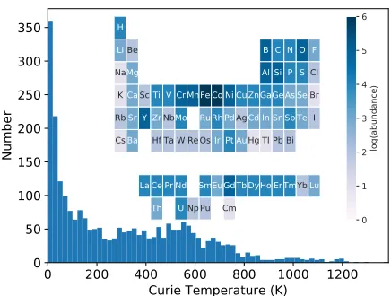
temperature. This means that typically a magnet will be considered as ‘useful’, if its Curie temperature is around 600 K. Unfortunately, not many magnetic compounds reach such value. In Fig. 1 we present the distribution of the measuredTC’s of about 2,500 known ferromagnets
(see later for details). The median of the distribution is 227 K, meaning that the vast majority of ferromagnets known to date are actually paramagnetic at room tem-perature. Furthermore, it is clear that the number of compounds satisfying the TC > 600 K criterion is only
∗[email protected] †[email protected]
a small fraction of the total, suggesting that finding new ‘useful’ ferromagnets is indeed a rare event and welcome news.
0 200 400 600 800 1000 1200 Curie Temperature (K)
0 50 100 150 200 250 300 350
Number
H
LiBe B C N O F
NaMg Al Si P SCl
KCaScTi V Cr MnFe Co Ni Cu ZnGaGe As SeBr
RbSr Y ZrNbMo RuRh PdAgCd In Sn Sb TeI
CsBa Hf Ta W Re OsIr Pt AuHg Tl Pb Bi
La Ce Pr Nd SmEuGdTb DyHo Er TmYbLu
Th UNp Pu Cm
0 1 2 3 4 5 6
[image:1.612.321.539.343.508.2]log(abundance)
FIG. 1. Histogram of theTC’s of about 2,000 known ferro-magnets. The median value of the distribution is 227 K. The insert shows the relative elemental abundance, in logarithmic scale, for the ferromagnets included in the dataset (the log-arithm of the number of compounds containing a particular element). The most frequent magnetic element is Co followed by Fe and Gd.
Figure1also presents the relative elemental abundance for the ferromagnets included in the dataset, namely for every element the number of compounds that contain that given element. As expected the vast majority of the ferromagnets contains at least one of the 3d magnetic transition metals, Fe, Co, Ni and Mn, with Al being the most frequent of the non-magnetic ions. However, it is interesting to note that, with the only exception of noble gases and highly radioactive elements, magnets can be made by incorporating essentially any ion in the periodic
table. This gives us a potentially very large chemical space to explore when designing new magnets.
In the last few years there have been a few attempts at systematically predicting the existence of new magnets ahead of experiments. These study are typically based on high-throughput numerical explorations [3], where the electronic structure of hypothetical compounds is com-puted at the level of density functional theory. The con-struction of the prototypes to calculate usually proceeds by substituting elements in known phases [4, 5], or by exploring the entire chemical space compatible with a given crystal structure [6]. In both cases one can ex-tract some elementary magnetic properties of the pro-totypes (magnetic moment per cell, density of states, magneto-crystalline anisotropy, etc.) and possibly assess their thermodynamical stability, namely one can forecast if a given prototype can be made and what its magnetic properties would be.
However, little information aboutTCcan be extracted,
unless the specific class of compounds investigated satis-fies some simple empirical rules. For example the Curie temperature of Heusler alloys of composition Co2XY,
withX andY being either a transition metal or a main group element, follows a Slater-Pauling curve [7], while Mn-containing magnets can be arranged along the phe-nomenological Castelliz-Kanomata curves [8, 9]. In the absence of such empirical rules the search for new com-pounds remains blind to TC. This is a rather severe
de-ficiency, since the calculations cannot distinguish from the outset which regions of the chemical space may yield high-TC magnets. As a consequence most of the
discov-ery computational effort is usually spent for materials with little technological potential.
Note that the prediction ofTCby first-principle
meth-ods is not an easy task either. The most common strategy consists in mapping electronic structure calculations onto some effective Hamiltonian, most typically the Heisen-berg model, which is then used to extractTC via Monte
Carlo techniques. This is a valid approach only if the rele-vant part of the magnetic excitation spectrum has a spin-wave nature, which is not universally guaranteed. As such the same method applied to different materials may result in predictions ofTC’s with a very different level of
agreement to experiments [10]. Certainly, the computa-tion of the entire magnetic excitacomputa-tion spectrum with den-sity functional theory is possible [11], but the computa-tional overheads are significant. Furthermore, also in this case uncertainty and errors arise from the choice of the exchange and correlation functional and from the other approximations taken. Overall, first-principle methods are very valuable for understanding the origin of a par-ticular TC, but they are currently not fit to be used as
a prediction tool ahead of experiments. For all these reasons it would be desirable to construct a universal predictor forTCbased solely on chemical information.
The present work responds to this demand. We intro-duce a range of machine-learning (ML) models, uniquely based on known experimental data for about 2,500
ferro-magnets, which can predict the Curie temperature using only chemical information. Machine learning is rapidly becoming a valuable tool in physics and materials science and it has been used already for a relatively wide range of problems. These go from the accelerated discovery of new materials [12, 13], to the estimation of materi-als physical quantities [14,15], to the definition of novel density functionals [16, 17]. Here we use ML to unveil patterns in the chemical-to-TC relation, and use these
patterns as predictors for theTC of new materials. Our
approach is in the same spirit of that used by Stanev and co-workers [18] to sort superconductors according to their critical temperature.
Our paper is structured as follows. Firstly, we intro-duce the computational methods used. In particular we discuss extensively the issues of representing the chemical composition of a given compound, of creating and pro-cessing the dataset, and of training and choosing the most appropriate and best performing ML model. We then discuss the performance of the various models against our dataset and show their ability to extrapolate in re-gions of data, where little information were available dur-ing the model traindur-ing. These, for instance, include the prediction of TC along the composition space of
differ-ent transition-metal binary systems and for the Al-Co-Fe ternary one. Finally we outline some possible ways to include information about the materials structure in the ML model and its effect on the overall accuracy.
II. METHODS
A. Definition of the feature vectors
The goal of supervised ML is to estimate a function, f, that maps a feature vector, x, to a target variable, y, namely to find the function f : x → y that better interpolates a set of available data (note that the target variable does not need to be a scalar quantity). In our case the feature vector contains information concerning a given compound, while the target variable isTC.
Al-though there are no rigorous stringent rules on how to construct the feature vector, ultimately the success of any ML strategy resides on the ability to define the most relevant features correlating to a given property. When the ML strategy is applied to materials science a number of desirable conditions defining the feature vector emerge naturally [14,19–22]. In particular it was proposed that the feature vector
1. should be computationally inexpensive to create. 2. should be continuous, reflecting the fact that the
properties of a material vary continuously.
4. should be able to distinguish different materials with different properties, namely different com-pounds with differentTCshould have different
fea-ture vectors.
We begin by defining feature vectors that do not include any structural information of compounds, but are con-structed to satisfy the first three conditions. Clearly the last one will be automatically violated, since polymorphs of a given chemical composition presenting differentTC’s
will be described by identical feature vectors. In particu-lar our goal is for the feature vectors to capture the ical composition of a given compound, namely its chem-ical formula. We can then divide the features defining a given compound into three categories: features which only take elemental properties into account (e.g. the atomic number), features which take only the compound stoichiometry into account, and features which take both into account.
Notably features belonging to the first category can be found to violate the second criterion and, for this reason, they have been excluded. Take as an example the max-imum atomic number, Zmax, of a given compound [23]
and consider the binary alloy A1−xBx, withZB> ZAas
an example. At x= 0 a feature vector containing this component will be discontinuous as the Euclidean dis-tance between A1and any A1−xBxwill always be greater
than|ZA−ZB|and will not go to zero smoothly asxgoes
to zero. In order to avoid this shortcoming we need to consider features that, either explicitly or implicitly, pre-serve information related to the atomic fractions of the various elements in a compound, and exclude those that just relate to the elemental properties. As such, features like the number of different elements in the compound (2 for binaries, 3 for ternaries, etc.) or the maximum atomic number are ruled out. In contrast a feature like the mode of the atomic number [24] is acceptable, since it encodes information about the atomic fractions.
Possible features created solely from the stoichiometry of a compound include the Lp stoichiometry norm [23]
and the stoichiometry entropy. The first one is gener-ally defined as||x||p = (Pi|xi|p)1/p, while the second is
S = −P
ixilog(xi), wherexi is the atomic fraction of
the i-th element. Features based on the product of the atomic fractions or on the number of different elements in the compound are ruled out by the second principle, using arguments similar to the one given above. In any case, one has still to establish whether stoichiometry-only features are informative enough for predicting most quan-tities.
Finally there are generally two ways to define features that take both elemental properties and stoichiometry into account. One possibility is to associate to each com-pound a high-dimension vector defined as
vchem={xH, xHe, xLi, xBe, ...} (1)
where xα is the atomic fraction of element α.
For instance, Fe3O4 is represented as the vector
(...,0,4/7,0, ...,0,3/7,0...), with 4/7 assigned at the eighth position (oxygen) and 3/7 to the 26th one (iron). The advantage of vchem is that it uniquely represents
a chemical formula, and its disadvantage that the vec-tors tend to be very sparse and high dimensional, hence difficult to train. A second option was suggested by Ward et al. [23] and consists in using composition-weighted elemental-properties. An example of these is the composition-weighted atomic number, defined as
hZi=P
iZixi, withZi andxi being the atomic number
and the atomic fraction of the elementi. In the case of Fe3O4this is 8(4/7)+26(3/7) = 15.71. Similar quantities
can be constructed with analogous definitions. Further-more, for any elemental quantity Qone can also define a composition-weighted mode h|Q|i, which takes the Q value of the element with the highest atomic fraction in the compound and an average in the case of multiple modes, and a composition-weighted absolute deviation
h∆Qi = P
i|Qi − hQi|xi. Table I summarises the
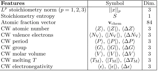
fea-tures used in this work.
Features Symbol Dim.
Lpstoichiometry norm (p= 1,2,3) ||x||p 3
Stoichiometry entropy S 1
Atomic fraction vector vchem 84
[image:3.612.318.579.291.409.2]CW atomic number hZi,h|Z|i,h∆Zi 3 CW valence electrons hNVi,h|NV|i,h∆NVi 3 CW period hPi,h|P|i,h∆Pi 3 CW group hGi,h|G|i,h∆Gi 3 CW molar volume hVi,h|V|i,h∆Vi 3 CW meltingT hTMi,h|TM|i,h∆TMi 3 CW electronegativity hi,h||i,h∆i 3
TABLE I. The full list of features used in this work. In the last column we report the dimension of any given feature. The atomic fraction vector has dimension 84, as not all elements in the periodic table can be found in the ferromagnets included in our database (e.g. He, Ar, etc.). In total our feature vector has a dimension of 129. Here “CW” denotes “composition-weighted”. The numerical values of the elemental properties are taken from Ref. [25].
B. Machine-learning models training
into three sets makes each one of them too small, dimin-ishing the overall ability of the model to learn and hence its accuracy. Therefore, in this case the training and the validation sets are combined into a single set, which we will refer to henceforth as the training set. ThenK-fold cross-validation is used to determine the hyperparame-ters and to select the best model. Here the training set is split intoK subsets (in this workK was chosen to be K = 3). For each given set the model is trained over the otherK−1 sets and tested over the remaining one, the cross-validation error is the average of all the errors. Then the best model, namely the model with the lowest cross-validation error, is trained over the entire training set. Finally, the test set is used to estimate the accuracy of the chosen model.
In order to quantify the model’s performance we have used the coefficient of determination,R2. Given a set of
target variables {yi}, with meanµ and predicted values
{f(xi)},R2 is given by
R2= 1−
P
i[y
i−f(xi)]2
P
i[yi−µ]2
. (2)
A perfect predictor of the target variables would always scoreR2= 1 on any set [f(xi) =yi for∀i].
C. Construction of the dataset
The dataset of experimentalTChas been constructed
by aggregating the following sources: the AtomWork database [27], Springer Materials [28], the Handbook of Magnetic Materials [29] and the book Magnetism and
Magnetic Materials [1]. A few additional values have
been taken from the references [30–32]. For a number of compounds the various databases report multiple val-ues ofTC, and there are also compounds where the same
database returns a range ofTC’s for the same
ferromag-net. Notably in the vast majority of cases the spread of TC’s about the mean is rather small, so that the choice
of a particular value is irrelevant. In particular, for 79% of the compounds associated to multipleTC’s the
differ-ence between the maximum and minimum value is less than 50 K. However, there is also a number of compounds presenting a much larger range of reported critical tem-peratures, namely for 4.9% of the multiple-TC data the
difference between the maximum and minimumTCvalue
is greater than 300 K.
There are several reason for these occurrences. In some compounds magnetism is subtly related to the quality of the sample, so that experiments performed by differ-ent groups may report differdiffer-entTC. This is particularly
relevant, since the various data sources containTC’s
ex-tracted over different periods of time, so that the spread of data sometime reflects the improvements in crystal growth over time. A second reason is related to polymor-phism, namely to the existence of compounds with the same stoichiometry but different crystal structure, and
hence differentTC. Finally, there are several
transition-metal/rare-earth intermetallic magnets for which mul-tiple TC are reported. For instance the two values of
186 K [33] and 641 K [34] have been both reported for Sm2Ni17. Such large discrepancy has been attributed
to the presence of possible secondary phases [34]. Since we are aiming at constructing ML models that use only chemical information to define compounds, our feature vector can not include any attribute related to sample quality or polymorphism. As such, in the presence of multipleTC’s we have to establish a criterion to select a
single value for any stoichiometry. In this work we have used the median of the distribution instead of the mean or the maximum value as this is more resistant to outliers. For instance, if for a given compound the reportedTC’s
are 300 K, 305 K and 700 K, their mean is 435 K while their median is 305 K. The first one is not associated to any real measurement while the second is.
In preparing our dataset we have carefully checked that there is enough diversity in the entries. Consider the fol-lowing thought experiment. Suppose that for every en-try in our database there are also many similar entries, namely there are several compounds with similar stoi-chiometry (feature vector) and similarTC. This may be,
for instance, the case of a binary alloy AxB1−x, where
many data are available in a narrow range of composi-tions. For a dataset of such homogeneous composition it is likely that almost any ML model will perform well. However, the same model will be unlikely to perform well for compounds significantly different to the ones found in the training set, namely the model will have little ability to generalize to a broader composition range. This is, of course, an unwanted feature. Our strategy to curate the database is then the following. Firstly, we standard-ise the chemical formula notation, by replacing fractional stoichiometry with integer one (e.g. Cu0.5Ni0.5 becomes
CuNi = Cu1Ni1), and by simplify the stoichiometry when
possible (e.g. Ni75Al25 becomes Ni3Al = Ni3Al1). At
this point we check for duplicates and, if these result in multipleTC’s for the same stoichiometry we take the
me-dian value. Next the dataset is ordered according to the number of atoms in the chemical formula and we com-pute the L1-norm of the atomic fraction vector, v
chem,
between all the entries in the database. If the distance between two entries is less than 0.01 we remove the com-pound with the larger number of atoms in its chemical formula. The rational for doing this reflects our intuition that Fe5Sn3and Fe8Sn5, with a distance of 0.019, should
be considered as two different compounds, while Co5Tb1
and Co5.1Tb1, with a distance of 0.005, are essentially
the same compound. In this last case we keep only the simpler Co5Tb1.
Finally our data needs to enable the ML models to dis-tinguish between magnetic and non-magnetic materials. This is not an issue if our only goal is that of describ-ing the TC of known ferromagnets, but it becomes one
when the ML model is used asTCpredictor for unknown,
dis-tribution, pdata, only includes ferromagnets, so that a
ML model will not be able to learn from pdata about
stoichiometries having TC = 0. A possible way out, as
suggested by Stanev et al. [18], is that of first training a classifier to predict whether or not a given compound has aTCgreater than some critical value,Tcritical. If one
sets Tcritical relatively low, the classifier will distinguish
between magnetic compounds and magnetic only at very low temperature. Here, however, we take a somewhat more straightforward approach and we simply include in our dataset some non-magnetic materials. In particular we include the elemental phases of all the non-magnetic elements of the periodic table. This procedure effectively provides to the ML model some information about non-ferromagnets and hopefully it makes it more robust when making new predictions.
After the data processing described above our train-ing set contains 1,866 entries, while the test set has 767. About 3% of the compounds are unaries, including the non-ferromagnetic ones. The ferromagnetic elemental phases are: Co (TC= 1380 K), Fe (1040 K), Ni (630 K),
Gd (290 K), Tb (220 K), Dy (85 K), Nd (30 K), Tm (30 K), Er (20 K), Ho (20 K) and Pr (8.7 K). Binaries and ternaries make up 31% and 49% of the dataset re-spectively with the rest of the dataset having more than 3 distinct elements.
III. RESULTS
A. Machine-learning model performance
In the construction of the ML models we compare four different algorithms, namely Ridge Regression (Ridge), Neural Network (NN), Kernel Ridge Regression (KRR) and Random Forests (RF). The NN is implemented em-ploying Keras [35], while for the rest we use Scikit-Learn [36]. For both Ridge and KRR the cross-validation set is used to determine the optimum regularization parameter. In contrast the dropout rate is the hyper-parameter used for the NN, while the maximum depth of the tree is that for RF. The accuracy of many algorithms can be some-times improved by reducing the dimension of the feature space. This is particularly true when there is correlation between the various features and for ML algorithms af-fected by the curse of dimensionality [37]. For a feature vector of dimensionp, one can construct 2p possible
sub-sets of the features, which in our case translates in∼1039
subsets [38]. It is, therefore, infeasible to perform an ex-haustive search for the best performing subset. Instead, we have decided to use two different methods of feature-dimension reduction, namely Correlation (C) and Princi-ple Component Analysis (PCA), and used such methods together with all the chosen ML algorithms. Correla-tion ranks the features according to the absolute value of the Pearson correlation coefficient, which is defined as cP = cov(x, y)/σxσy, with cov(x, y) being the (x, y)
co-variance and σthe standard deviation. In our case y is
theTC and x corresponds to each feature. In contrast,
the PCA projects the feature space into a lower dimen-sional one, while trying to preserve as much data variance as possible [39].
The results of the 3-fold cross validation score for the different algorithms operated together with different fea-ture reduction techniques are shown in TableII. In
gen-R2 All C10 C20 C40 C80 P10 P20 P40 P80 Ridge 0.53 0.48 0.5 0.52 0.52 0.24 0.27 0.31 0.39 KRR 0.69 0.72 0.72 0.72 0.69 0.69 0.72 0.70 0.68 NN 0.76 0.72 0.76 0.77 0.78 0.73 0.77 0.77 0.77 RF 0.81 0.76 0.77 0.78 0.79 0.72 0.74 0.73 0.72
TABLE II. 3-fold cross-validation R2 score of all the algo-rithms chosen combined with the various feature reduction techniques. “All” indicates the case where no feature reduc-tion is applied. “C” means Correlareduc-tion feature reducreduc-tion and “P” is for PCA. The number beside the type of feature re-duction scheme indicates the size of the reduced feature space. Thus, for example, P40 means that PCA has generated a 40-dimensional feature space.
eral we find that the performance of the different algo-rithms ranks them in the following order Ridge, KRR, NN and RF. Dimensionality reduction does not seem to significantly improve the R2 and in fact, with the only
exception of the Correlation scheme applied to KRR and NN, it appears always better to run the ML algorithm over the full feature space. Overall Random Forests using the entire set of features performs the best on the cross-validation sets and, therefore, it is chosen as the final model. RF achieves a cross-validationR2 of 0.81 and a
test one of 0.87, demonstrating that the cross-validation score is a good estimate of the test error.
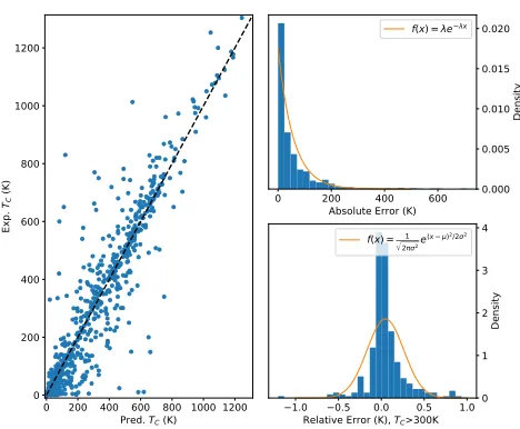
In Fig. 2 we present our best result for the RF algo-rithm. Here we plot the predictedTC’s against the
ex-perimental ones for all the ferromagnets contained in the test set. In addition we present a distribution of the ab-solute errors and one for the relative error of compounds presentingTC>300 K. In general we find that our ML
model can predict relatively well the experimentalTC, in
particular for Curie temperatures exceeding 300 K. This is important since in this range one finds the magnets useful for room-temperature applications. The mean ab-solute error over the entire distribution is 57 K. Such a value gives us confidence that the ML model can dis-tinguish between high-TCferromagnets and low-TCones,
namely it allows us to identify the potential of an hypo-thetical chemical composition against ferromagnetism.
The distribution of theTCabsolute errors for our best
ML model is exponential with decay coefficient, λ, of 0.018. From the distribution one can learn that an 1−e−λx fraction of the data are with x K of the ex-perimental data. For example 59 % of the predictedTC’s
are within 50 K from the measured ones, and 83 % are within 100 K. Large absolute errors are found only for compounds presenting a rather smallTC, which are
de-0 200 400 600 800 1000 1200 Pred. TC (K)
0 200 400 600 800 1000 1200
Ex
p.
TC
(K
)
0 200 400 600
Absolute Error (K)
0.000 0.005 0.010 0.015 0.020
Density
f(x) = e x
1.0 0.5 0.0 0.5 1.0
Relative Error (K), TC>300K
0 1 2 3 4
Density
f(x) = 1
2 2e(x )
2/22
FIG. 2. RF model for the TC of ferromagnets. In the left-hand side panel we compare the experimental and predicted
TCfor the test set. TheR2coefficient of the model is 0.87 and the mean absolute value is 57 K. The upper left panel shows the distribution of absolute errors,|TCexp−TCpredic|, while the lower one displays the distribution of the relative errors for compounds with TC>300 K. The orange lines indicate the best fit respectively to an exponential and a Gaussian distri-bution.
tailed understanding of the performance of our ML model can be obtained by looking at the distribution of the rel-ative error, defined as (TCexp−TCpredic)/TCexp, whereTCexp andTCpredic are respectively the average experimentalTC
and the predicted one. In this case we present data only for compounds withTCexceeding 300 K (right-hand side
panel of Fig.2). There are two main reasons behind such choice. On the one hand, these are the compounds poten-tially useful for room-temperature applications. On the other hand, for ferromagnets presenting low measured TC, relative small absolute errors may result in rather
large relative ones. In this case the distribution appears symmetric around zero, indicating that our ML model has no systematic bias towards either overestimating or underestimating TC. The shape of the distribution is
Gaussian-type with a half-height width of 0.51. We find that only 5 % of the compounds present a relative error larger than 50 %, and only 15 % have errors larger than 25 %.
Finally we take a look at whether or not our ML model tends to systematically fail for some particular chemical compositions. Again we analyse data only for compounds withTC>300 K. In Table IIIwe present the elemental
abundance, fα
M, of the most relevant magnetic
transi-tion metals, M, among compounds presenting a relative error beyond a give threshold, α. For instance, in the cell corresponding to f50
M and Cr we show the relative
abundance of the Cr element among the compounds pre-senting a predictedTC with a relative error larger than
50 %,f50
Cr. The abundance is calculated as the total
num-ber of compounds presenting a given element divided by the total number of compounds. Note that the elemental abundances do not necessarily sum up to unity, since a compound may contain more than one transition metal.
Element fM50 fM30 fM20 fM10 fM5 fM2 fM0
[image:6.612.59.293.51.244.2]Cr 0.0 0.01 0.02 0.02 0.04 0.05 0.05 Mn 0.02 0.04 0.08 0.09 0.12 0.14 0.15 Fe 0.03 0.07 0.13 0.24 0.38 0.56 0.74 Co 0.01 0.02 0.03 0.06 0.11 0.17 0.21 Ni 0.01 0.02 0.02 0.03 0.04 0.05 0.05 Total 0.05 0.13 0.21 0.36 0.56 0.79 1.0
TABLE III. Elemental abundance,fα
M, of the most relevant
magnetic transition metals,M, among compounds presenting a relative error beyond a give threshold,α (in %). The last row, labelled as ‘total’, lists the fraction of compounds with errors exceedingα (e.g. 0.13 of the compounds have a pre-dictedTCwith error exceeding 30%). The last column (error 0 %) shows the elemental abundance over the entire set.
In general, as expected, we find that the elemental abundance grows as the error on the predictedTC gets
smaller. Such dependence is rather flat for Cr, Mn and Ni, mostly because a relatively limited number of com-pounds containing these three transition metals are found ferromagnetic above 300 K. The distribution of errors is thus dominated by Fe-containing, and partially Co-containing, ferromagnets, which are calculated with an accuracy comparable to that of the total set. We can then conclude that our best ML model is well balanced across chemical composition and does not favour any par-ticular region of the chemical space.
B. Ability of the model to extrapolate
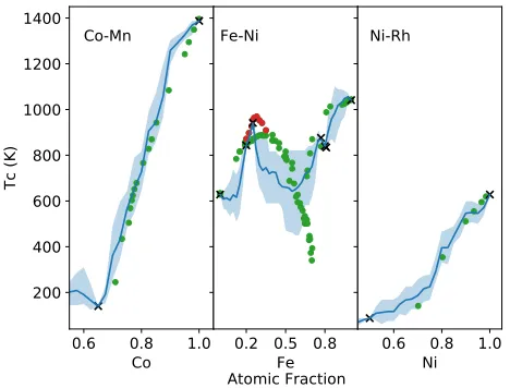
Next we demonstrate the ability of our model to ex-trapolate to regions of the chemical space where only a few data points were present in the training set. Our first example consists in predicting theTCas a function
the confidence interval of the random forest algorithm (light-blue shadow).
0.6
0.8
1.0
Co
200
400
600
800
1000
1200
1400
Tc (K)
Co-Mn
0.2 0.5 0.8
Fe
Fe-Ni
0.6 0.8 1.0
Ni
Ni-Rh
[image:7.612.60.294.95.273.2]Atomic Fraction
FIG. 3. TC prediction as a function of composition for three binary transition-metal systems, namely Co-Mn, Fe-Ni and Ni-Rh. Data are presented as a function of the atomic frac-tion of one of the two species. The blue line traces the ML prediction, black crosses (green dots) are experimental points included (not included) in the training set. The experimen-tal results are taken from references [40–42]. The light-blue shadowed area corresponds to the range of predictedTC’s of subsets of the trees, namely it indicates the uncertainty of the ML model. In the middle panel the red dots correspond to theTCassociated to the FeNi3 intermetallic phase, while the
green ones correspond to random Ni-Fe alloys.
Manganese and cobalt can form disordered alloys with a few possible crystal structures across the entire com-position range [43]. The magnetic phase diagram was determined sometime ago [40] and comprises both fer-romagnetic and antiferfer-romagnetic orders. In particular when the Co atomic fraction is larger than about 0.68 the alloys are ferromagnetic with aTCthat monotonically
in-creases as a function of the Co content. In contrast, Mn-rich alloys are antiferromagnetic with a N´eel temperature that this time monotonically increases as the Mn concen-tration gets larger. Our ML model predicts well the TC
for all the ferromagnetic phases, with a constant minimal error. For this case only two data points were included in the training set, namely elemental Co and the end-of-the-series alloy, Co13Mn7. Intriguingly, the model seems
to be able to predict also the upturn in critical temper-ature occurring for Co atomic fractions lower than 0.68, although these correspond to antiferromagnetic phases. It is worth noting that the spread of values returned by the RF algorithm is certainly larger for these Mn-rich phases.
The Ni-Fe system presents a different level of complex-ity, with the ferromagnetic order being present over the entire composition range [41]. In the region of tempera-tures relevant forTC the Fe-rich phases (for a Fe atomic
fraction down to 0.65) are characterized by Ni-dopedbcc
iron with a TC that grows monotonically as a function
of the Fe fraction. In contrast, when the Fe atomic frac-tion is reduced below 0.65 the relevant phase is an fcc random alloy, which can be stabilized up to bulk Ni. In this case theTC is non-monotonic, it increases with the
Ni atomic fraction up to 0.70 (the maximumTCis about
870 K for Fe30Ni70) and then it decreases down to the TC of bulk Ni. Furthermore, there is also an ordered
intermetallic FeNi3 ferromagnetic phase, which persists
over a relatively narrow composition range. This means that in Fe1−xNix at x ∼ 0.75 there are two
ferromag-netic phases with different TC’s. Also in this case our
ML model performs rather well. This time seven experi-mental data points were included in the training set, two for the elemental Ni and Fe and five across the Fe1−xNix
alloys. In particular the composition corresponding to the maximum at the intermetallic FeNi3 phase was
in-cluded. Our ML model interpolates well between these points, in particular in the Ni-rich part of the composi-tion diagram. As expected from the fact that structural information are not included in the model, we are not able to distinguish the differentTC’s associated to
differ-ent structures.
Finally, we look at the Ni-Rh binary system, an alloy where only one of the two elements is magnetic. As with several other elements of the Pt group, Rh is highly sol-uble in Ni and random alloys can be formed over almost the entire composition range. Here theTCmonotonically
decreases from that of bulk Ni as Rh is added to the al-loy. This continues up to a critical composition, found for a Ni atomic fraction of around 63%, where the ferro-magnetism disappears completely [44]. Our ML model is fully capable of describing such behaviour. In particular the ML model successfully predicts the critical concentra-tion for the suppression of ferromagnetism at a Ni atomic fraction lower then 0.7. This is a rather compelling re-sult.
As a second example of the ability of our ML model to extrapolate to unexplored regions of the chemical space we present the TC diagram of the ternary system
Al-Co-Fe. In Fig. 4 we show the TC across the ternary
composition space as a colour-coded heat map and that across the three possible binary systems as a standard graph, similar to those of Fig. 3. Also in this case for the binary systems we represent the data included in the training set as black crosses and those outside the train-ing set as solid dots. The same convention is adopted for phases in the middle of the ternary diagram, where now the data included in the training set are solid square. Note that this ternary system includes three stoichiomet-ric magnetic phases, namely Co2FeAl [46], Fe2CoAl [47]
and Fe3Al [48]. Furthermore, magnetic solid state
solu-tions can be stabilized over a rather large composition space.
0.0 0.2 0.4
0.6 0.8
1.0
0 250 500 750 1000 1250
Tc (K)
0.0
0.2
0.4
0.6
0.8
1.0 0
250500
750
10001250
Tc (K)
0.0 0.2
0.4 0.6
0.8 1.0
0 250 500 750 1000 1250
Tc (K)
T
CFe
Co
Al
1
2
3
Atomic F
rac tion Al
Atomic F rac
tion F e
[image:8.612.153.517.72.362.2]Atomic Fraction Co
FIG. 4. TCprediction as a function of composition for the ternary system Al-Co-Fe. Data are presented as a function of the atomic fraction of the three species and theTCis expressed as a heat map. The figure also introduces a detailed analysis of the three relevant binary phase diagrams, where the blue line traces the ML prediction, black crosses (green dots) are experimental points included (not included) in the training set. The light-blue shadowed area in the binary plots corresponds to the range of predictedTC’s, namely it indicates the uncertainty of the ML model. The solid square (circles) included in the ternaryTC
diagram are for experimental data included (not included) in the training set, with the colour code describing theTC. Numbers correspond to three known stoichiometric phases: 1) Co2FeAl,TC= 1,000 K, 2) Fe2CoAl,TC>873 K, 3) Fe3Al,TC= 573 K.
The plot was partially made using python-ternary [45].
the fact that only a rather limited number of compounds across the various phase diagrams were included in our training set. For instance, the model is capable of de-scribing the critical Al concentration for the appearance of ferromagnetism in Al-Co [49], which has been mea-sured to be at an Al atomic fraction of about 50%. In this case only the end points of the composition diagram, namely elemental Co and Al, were present in the train-ing set, so that the ML model is able to extrapolate such critical concentration from the learning obtained in other part of the chemical space.
The case of Al-Fe is relatively more complex. Our ML model is trained with only three data points from this binary system, namely the end points and the Fe3Al
sto-ichiometric phase. The resulting TC-versus-composition
curve then predicts a monotonic reduction of the Curie temperature as the Al atomic fraction increases, with a rather smooth approach toTC= 0 for pure Al.
Experi-mental data obtained for rf-sputtered thin films display a well-disorderedbccphase for Al atomic fractions up to
70%, followed by an amorphous phase between 75% and 85%, and then by anfcc phase for higher Al fractions. The disordered bcc phases are all ferromagnetic, while both the amorphous and thefccones are paramagnetic down to 4.2 K [50]. Although the precise position of such phase boundaries seems to depend somewhat on the de-tails of the growth conditions [51], our ML model appears also in the case to be able to capture such behaviour.
At variance with the Al-Fe and Al-Co case, the TCof
the Co-Fe binary system presents a non-monotonic be-haviour with composition. As we move from elemental Co to elemental Fe, first theTC decreases with
increas-ing the Fe content, up to a Fe atomic fraction of around 30%. In this case the magnetic transition takes place within the Co-Fe γ-phase (fccstructure). Then, for Fe atomic fractions comprised between ∼30% and ∼80%, TCfirst increases and then decreases, reaching up a
com-position range, for Fe atomic fractions above 80%, TC
keeps decreasing down to that of elemental Fe, but the alloys remain in theαphase, namely the magnetic phase transition no longer traces the structural phase boundary [52].
Finally, we take a look at the TC’s for the ternary
phases, namely in the center of the composition dia-gram. In this case no experimental information was in-cluded in the training set. Two ternary stoichiometry compounds are known for Al-Co-Fe, namely the Heusler alloys Co2FeAl and Fe2CoAl. Their Curie temperature
are 1,000 K for Co2FeAl [46] and at least 873 K for
Fe2CoAl [47] (TC has not been measured with precision
and only a lower bound is available). Our ML model predicts respectively 657 K and 580 K, hence it provides an underestimation of the real TC’s, although it ranks
the materials in the right order. Additional experimen-tal data are available across the Al-Co composition (for an Al atomic fractions not exceeding 30%) and constant Fe atomic fractions of 30% and 50% [53]. These data are reported as full circles in Fig. 4 showing the ability of our ML model to describe the general trend, namely a decrease inTCas the Al atomic fraction increases. Also
in this case some non-monotonicity is found in the exper-imental data for small Al concentrations, which is asso-ciated to the fact that for such composition range theTC
traces the phase boundary between theαandγ phases. Our ML model appears to be able to trace such non-monotonicity.
C. Incorporating structural information in the
feature vector
As constructed, our ML model does not include any information about the atomic structure of a given com-pound. For this reason it is unable to distinguish the Curie temperatures of two polymorphs having the same chemical composition, a fact that has been discussed in connection to the Ni-rich part of the Fe-Ni TC diagram
(see Fig.3). We now present an attempt at overcoming such shortfall by including structural information in our feature vector. This is not a trivial task.
Several strategies to encode structural information of materials in a way that satisfies the four criteria intro-duced in the Method section have been proposed. These include partial radial distribution functions [54], Voronoi tessellation [55] and representations learnt by neural net-works [56]. The issue with including structural informa-tion is that it massively increases the size of the input space, thus requiring much more training data to fully capture the space. This may not be a problem when data is abundant or can be easily generated, but it be-comes one when the data is limited, as in our case. In fact, out of our entire dataset, only 792 entires have an associated entry in the ICSD database [57]. As such only this subset of data can be used in a ML model informed by structural parameters.
We have then constructed four different ML models, each one of them containing only a limited description of the structural information of a compound. The first, denoted as Original + Volume, associates to any com-pound, in addition to the previous features, the unit cell volume per atom. The second one replaces the atomic fraction of each element present in a compound with its volume fraction, defined asvchem·V, whereV is the
vol-ume per atom of the material. This is denoted as Orig-inal with V-Frac. The next two models, instead, include a more detailed representation of the atomic positions. We have taken inspiration from the work of Sch¨utt et al. [54], who introduced structural information in the form of a radial distribution function,
f(r) = 1 Ncell
Ncell
X
i=1
X
j
θ(dij−r)θ(r+ ∆−dij). (3)
Here Ncell is the number of atoms in the unit cell, the
index i runs over all the atoms in the unit cell, while the indexj over all the atoms neighbouring that atiare within some distance cutoff, θ(x) is the Heaviside step function,dij is the distance between the atoms i and j
and finally ∆ is the interval, a parameter that we must specify. Note that θ(dij −r)θ(r+ ∆−dij) is equal to
one if r < dij < r+ ∆ and vanishes otherwise. In our
case we evaluate f(r) at the points rn =n∆, where n
is an integer, and the resulting function is added to the original feature vector (Original + f model).
A second strategy, which tries to incorporate more in-formation in the radial distribution function consists in defining an “interaction-resolved radial distribution func-tion”
fα(r) =
1 Ncell
Ncell
X
i=1
X
j
θ(dij−r)θ(r+ ∆−dij)δα,ij. (4)
Hereαrepresents a type of “interaction” and δα,ij does
not vanish, if the atoms at the positions i and j define that given interaction. In practice, with “TM” meaning a transition metal atom, “LA” a lanthanide, and “OT” an atom of other type, we consider six types of interactions: TM-TM, TM-LA, TM-OT, LA-LA, LA-OT and OT-OT. Thus, the fα(r) radial distribution function effectively
defines the type-specific neighbourhood of a given atom. Note that the two distribution functions are related to each other by the sum rulef(r) =P
αfα(r). The
ratio-nale behindfαis that the magnetic exchange interaction
is, in general, dependent on the atom type, and deter-mines theTC. As such, by containing the fαour feature
vector is expected to have some freedom to learn about the exchange interaction of a given compound. A similar, although more complex, representation was used also by Sch¨utt et al. [54]. Here we have simplified the description to keep the dimension of the feature vector relatively low. This last model is denoted asOriginal + fab.
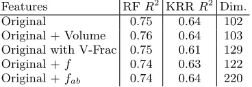
that on this reduced data subset the original feature vec-tor (129-dimensional) is not able to generate ML models as accurate as before. For instance the R2 coefficient of
the RF algorithm is now only 0.75, compared with the previous value of 0.81. This is expected, since the pool of data used for the construction of the model now has been drastically reduced. Unfortunately, we also find that any additional feature added to the original vector generally makes the construction of an accurate ML model less suc-cessful with R2 coefficients systematically smaller than
those obtained for the original model regardless of the specific ML algorithm used. The exception here is when adding the volume as a feature. However, the improve-ment is so small that it is doubtful whether this is a significant result. There are two possible reasons, prob-ably both at play, behind this result. Firstly, in all cases the feature vector dimension is larger, while the training dataset is smaller. Thus the models have now less data to train but more information to use, effectively jeopar-dising their ability to learn. Secondly, we have now little control on the balance of the data, meaning that we may have a disproportionated amount of information across the different regions of the chemical space.
Features RFR2 KRRR2 Dim.
Original 0.75 0.64 102
[image:10.612.86.270.328.392.2]Original + Volume 0.76 0.64 103 Original with V-Frac 0.75 0.61 129 Original +f 0.74 0.63 122 Original +fab 0.74 0.64 220
TABLE IV. The 3-fold cross-validationR2 score of the vari-ously defined feature vectors for both Random Forests (RF) and Kernel Ridge Regression (KRR). Note that here “Orig-inal” refers to the original set of features. The last column reports the dimension of the feature vector.
IV. CONCLUSION
We have here described the construction of a ML model to predict the Curie temperature of ferromagnets solely based on their chemical composition. The model has been entirely trained over available experimental data and its construction did not involve any electronic struc-ture calculations. We have considered several ML algo-rithms and, by using Random Forest we have been able to generate a model presenting a mean absolute error of only 57 K over a test set containing 767 compounds. Interestingly most of the error is associated to magnets with low TC, so that the model is capable to identify
high-TC ferromagnets.
We have then made several attempts to include struc-tural information into the description, but we have never been able to outperform the models containing chemical data only. This is likely to be related to the smaller pool of data to use for the training and to the larger dimen-sion of our feature space. It is also interesting to note that ferromagnets, being mostly metallic, are less sensi-tive than other magnetically ordered compounds to the structural details. All in all our ML model can be viewed as a first rough guide to navigate the chemical space of magnetism, namely as a first step toward a ML-driven magnetic materials discovery strategy.
Acknowledgment
Financial support for this work has been provided by the Irish Research Council. We thanks Alessandro Lunghi for useful discussions and for a critical read of the manuscript.
[1] J. Coey,Magnetism and magnetic materials (Cambridge University Press, 2010).
[2] S. Blundell, Magnetism in condensed matter (Oxford Univ. Press, 2001).
[3] S. Curtarolo, G. L. W. Hart, M. B. Nardelli, N. Mingo, S. Sanvito, and O. Levy, Nature Materials 12, 191 (2013).
[4] J. M¨oller, W. K¨orner, G. Krugel, D. Urban, and C. Els¨asser, Acta Mater.153, 53 (2018).
[5] W. K¨orner, G. Krugel, D. Urban, and C. Els¨asser, Scripta Mater.154, 295 (2018).
[6] S. Sanvito, C. Oses, J. Xue, A. Tiwari, M. Zic, T. Archer, P. Tozman, M. Venkatesan, J. Coey, and S. Curtarolo, Sci. Adv.3, e1602241 (2017).
[7] T. Graf, C. Felser, and S. S. P. Parkin, Prog. Solid State Chem.39, 1 (2011).
[8] L. Castelliz, Z. Metallk.46, 198 (1955).
[9] T. Kanomata, K. Shirakawa, and T. Kaneko, J. Magn. Magn. Mater.65, 76 (1987).
[10] I. Turek, J. Kudrnovsky, V. Drchal, and P. Bruno, Phil. Mag.86, 1713 (2006).
[11] P. Buczek, A. Ernst, P. Bruno, and L. M. Sandratskii, Phys. Rev. Lett.102, 247206 (2009).
[12] G. Pilania, C. Wang, X. Jiang, S. Rajasekaran, and R. Ramprasad, Sci. Rep.3, 2810 (2013).
[13] B. Meredig, A. Agrawal, S. Kirklin, J. E. Saal, J. Doak, A. Thompson, K. Zhang, A. Choudhary, and C. Wolver-ton, Phys. Rev. B89, 094104 (2014).
[14] M. Rupp, A. Tkatchenko, K.-R. M¨uller, and O. A. Von Lilienfeld, Phys. Rev. Lett.108, 058301 (2012). [15] O. Isayev, C. Oses, C. Toher, S. C. Eric Gossett, and
A. Tropsha, Nature Comm.8, 15679 (2017).
[16] J. C. Snyder, M. Rupp, K. Hansen, K.-R. M¨uller, and K. Burke, Phys. Rev. Lett.108, 253002 (2012).
[17] J. Nelson, R. Tiwari, and S. Sanvito, Phys. Rev. B99, 075132 (2019).
[18] V. Stanev, C. Oses, A. G. Kusne, E. Rodriguez, J. Paglione, S. Curtarolo, and I. Takeuchi, npj Comp. Mat.4, 29 (2018).
[20] A. Jain, G. Hautier, S. P. Ong, and K. Persson, J. Mat. Res.31, 977 (2016).
[21] F. Faber, A. Lindmaa, O. A. von Lilienfeld, and R. Armiento, Int. J. Quant. Chem.115, 1094 (2015). [22] O. A. von Lilienfeld, R. Ramakrishnan, M. Rupp, and
A. Knoll, Int. J. Quant. Chem.115, 1084 (2015). [23] L. Ward, A. Agrawal, A. Choudhary, and C. Wolverton,
npj Comp. Mat.2, 16028 (2016).
[24] The mode of the atomic number of a compound is defined as the atomic number of the most abundant element of that compound. For example, the atomic number mode of Fe3O4 is 8, the atomic number of oxygen. In case two
or more elements have maximal abundance the mode is defined as the average of their atomic numbers.
[25] S. P. Ong, W. D. Richards, A. Jain, G. Hautier, M. Kocher, S. Cholia, D. Gunter, V. L. Chevrier, K. A. Persson, and G. Ceder, Comp. Mat. Sci.68, 314 (2013). [26] J. Friedman, T. Hastie, and R. Tibshirani,The elements of statistical learning, 2nd ed. (Springer Series in Statis-tics, 2009).
[27] Y. Xu, M. Yamazaki, and P. Villars, Jpn. J. App. Phys.
50, 11RH02 (2011).
[28] T. F. Connolly, Bibliography of magnetic materials and tabulation of magnetic transition temperatures (Springer Science & Business Media, 2012).
[29] K. Buschow and E. Wohlfarth, eds.,Handbook of Mag-netic Materials, Volumes 4-16 & 18 (Elsevier, 1988-2009).
[30] H. Albert and L. Rubin, Advances in Chemistry series
98, 1 (1971).
[31] F. Givord and R. Lemaire, Solid State Commun.9, 341 (1971).
[32] H. Okamoto, Bulletin of Alloy Phase Diagrams10, 549 (1989).
[33] P. D. Carfagna and W. Wallace, J. Appl. Phys.39, 5259 (1968).
[34] K. Buschow, Rep. Prog. Phys.40, 1179 (1977). [35] F. Cholletet al., “Keras,”https://keras.io(2015). [36] F. Pedregosa, G. Varoquaux, A. Gramfort, V. Michel,
B. Thirion, O. Grisel, M. Blondel, P. Prettenhofer, R. Weiss, V. Dubourg, J. Vanderplas, A. Passos, D. Cour-napeau, M. Brucher, M. Perrot, and E. Duchesnay, J. Mach. Learn. Res.12, 2825 (2011).
[37] R. Bellman,Dynamic Programming, Rand Corporation research study (Princeton University Press, 1957).
[38] The value provided here is calculated over all possible feature subsets, regardless of the dimensionality of the associated feature space.
[39] I. Goodfellow, Y. Bengio, and A. Courville,Deep learn-ing (MIT press, 2016).
[40] A. Menshikov, G. Takzei, Y. A. Dorofeev, V. Kazantsev, A. Kostyshin, and I. Sych, Zh. Eksp. Teor. Fiz.89, 1269 (1985).
[41] L. Swartzendruber, V. Itkin, and C. Alcock, J. Phase Equilib.12, 288 (1991).
[42] J. Crangle and D. Parsons, Proc. R. Soc. London A255, 509 (1960).
[43] K. Ishida and T. Nishizawa, Bulletin of Alloy Phase Di-agrams11, 125 (1990).
[44] W. C. Muellner and J. S. Kouvel,Phys. Rev. B11, 4552 (1975).
[45] M. Harper, B. Weinstein, C. Simon, et al., “Python-ternary: ternary plots in python. zenodo,” (2015). [46] T. Graf, C. Felser, and S. Parkin, Prog. Sol. State Chem.
39, 1 (2011).
[47] M. Yin, P. Nash, and S. Chen, Intermetallics 57, 34 (2015).
[48] R. Nathans, M. Pigott, and C. Shull, J. Phys. Chem. Solids6, 38 (1958).
[49] A. McAlieter, Bulletin of Alloy Phase Diagrams10, 646 (1989).
[50] M. Shiga, T. Kikawa, K. Sumiyama, and Y. Nakamura, J. Magn. Soc. Jpn. Mag.9, 187 (1985).
[51] K. Sumiyama, Y. Hirose, and Y. Nakamura, J. Phys. Soc. Jpn.59, 2963 (1990).
[52] T. Nishizawa and K. Ishida, Bulletin of Alloy Phase Di-agrams5, 250 (1984).
[53] V. Raghavan, J. Phase Equilib. Diff.26, 57 (2005). [54] K. Sch¨utt, H. Glawe, F. Brockherde, A. Sanna, K. M¨uller,
and E. Gross, Phys. Rev. B89, 205118 (2014).
[55] L. Ward, R. Liu, A. Krishna, V. I. Hegde, A. Agrawal, A. Choudhary, and C. Wolverton, Phys. Rev. B 96, 024104 (2017).
[56] K. T. Sch¨utt, H. E. Sauceda, P.-J. Kindermans, A. Tkatchenko, and K.-R. M¨uller, J. Chem. Phys.148, 241722 (2018).