University of Southampton Research Repository
ePrints Soton
Copyright © and Moral Rights for this thesis are retained by the author and/or other
copyright owners. A copy can be downloaded for personal non-commercial
research or study, without prior permission or charge. This thesis cannot be
reproduced or quoted extensively from without first obtaining permission in writing
from the copyright holder/s. The content must not be changed in any way or sold
commercially in any format or medium without the formal permission of the
copyright holders.
When referring to this work, full bibliographic details including the author, title,
awarding institution and date of the thesis must be given e.g.
AUTHOR (year of submission) "Full thesis title", University of Southampton, name
of the University School or Department, PhD Thesis, pagination
UNIVERSITY OF SOUTHAMPTON
FACULTY OF ENGINEERING AND APPLIED SCIENCE MECHANICAL ENGINEERING DEPARTMENT
"NUMERICAL METHODS FOR STRESS ANALYSIS USING KNOWN ELASTICITY SOLUTIONS"
by
A.R. Carmichael
Being a thesis submitted for the degree of Doctor of Philosophy
CONTENTS
ABSTRACT
Page iv.
ACKNOWLEDGEMENTS V .
NOTATION: (Part I) (Part Ii;
V I .
X .
LIST OF FIGURES X I V .
LIST OF TABLES
CHAPTER 1. GENERAL INTRODUCTION
1.1 Background to the work
1.2 Review of theoretical methods and solutions 1.2.1 Exact analytical methods
1.2.2 Approximate analytical methods 1.2.3 Numerical methods
1.3 Layout of thesis
1 4 4 5 7 11
PART I Finite Element Superposition Method
CHAPTER 2. FINITE ELEMENT FORMULATION
2 .1 Introduction 13
2 .2 Notation for the boundaries 14
2 .3 Displacement and stress fields 16
2, .4 The variational ] principle 19
2, ,5 Determination of correction stress field 0 . c
—1 22
2. 6 Determination of the nodal displacements 24 2. 7 Determination of the trial function coefficients 26 2. 8 Determination of the stress at any point 29
2. 9 Summary 30
CHAPTER 3. TRIAL FUNCTIONS AND LOADING FUNCTION
3.1 Introduction
3.2 Trial functions for elliptical holes
Page
3.3 Trial functions for circular holes 3.4 Loading function for circular holes
33 39
CHAPTER 4. IMPLEMENTATION OF FINITE ELEMENT METHOD
4.1 Introduction
4.2 Structure of Program 4.2.1 Data input
4.2.2 Areas of elements 4.2.3 Stiffness matrix
4.2.4 Trial and loading functions 4.2.5 Stress fields of
4.2.6 Boundary conditions 4.2.7 Strain energy term 4.2.8 Correction to matrix D 4.2.9 Solution of the equations 4.2.10 Trial function coefficients 4.2.11 Displacements and stresses 4.3 Using the Program
42 42 44 44 45 45 45 46 46 46 48 48 48
48
CHAPTER 5. FINITE ELEMENT RESULTS
5.1 Introduction 50
5.2 Rectangular plate with central traction-free hole 51
5.2.1 Effect of mesh refinement 53
5.2.2 Effect of hole size 54
5.2.3 Effect of hole aspect ratio 56
5.2.4 Effect of special region size and additional
trial functions 60
5.2.5 Effect of local mesh refinement 67
5.3 Square plate with central traction-free hole 69
5.3.1 Circular hole 69
5.3.2 Elliptical hole 72
5.4 Configurations with loaded circular holes 76 5.4.1 Various loadings on a circular hole 77 5.4.2 Pressurized hole in annulus or large plate 92
5.4.3 Symmetrical rectangular lug 93
5.4.4 Rectangular lugs 98
PART II Modified Boundary Element Method
CHAPTER 6. BOUNDARY ELEMENT FORMULATION
6.1 Introduction 6.2 Notation
Page
6.3 Basis of the boundary element method 109
6.4 Discretization of the equations 111
6.5 Solution of the equations 113
6.6 Interior points 113
6.7 Modified kernel function 115
6.8 Implementation 117
CHAPTER 7. BOUNDARY ELEMENT RESULTS
7.1 Configurations analysed 119
7.2 Comparison between modified and standard kernel
functions 120
7.3 Annuli with various sizes of hole 123
7.4 Square plates with various sizes of hole 125
CHAPTER 8. GENERAL CONCLUSIONS
8.1 The finite element superposition method 128
8.2 The modified boundary element method 131
8.3 Comparison of the methods 132
8.4 Future work 133
REFERENCES 136
APPENDIX A. Derivation of the variational principle 154
APPENDIX B. Listings of selected program segments (FESM) 157
APPENDIX C. Data preparation for finite element program 174
APPENDIX D. Running the finite element program 181
APPENDIX E. Finite element meshes 196
APPENDIX F. Modified fundamental solution 202
UNIVERSITY OF SOUTHAMPTON
ABSTRACT
FACULTY OF ENGINEERING AND APPLIED SCIENCE
MECHANICAL ENGINEERING
Doctor of Philosophy
NUMERICAL METHODS FOR STRESS ANALYSIS USING KNOWN ELASTICITY SOLUTIONS
by Andrew Robert Carmichael
Two methods for the determination of the stress concentration near holes in two dimensional elastic components are developed. One, which is based on the finite element method extends a superposition technique originally developed for crack problems; the other uses the boundary element method. Both methods involve using analytical solutions which satisfy conditions on the hole boundary exactly thereby reducing or, in the case of boundary elements avoiding entirely, the need for elements modelling the hole.
The first method uses a modified complementary energy functional to determine the coefficients of the superimposed functions and the finite element nodal displacements, from which the estimates of stress are obtained. Tractions on the hole boundary are represented accurately using Fourier series, and the formulation is modified by the inclusion of a "loading function" which is the solution for an infinite region containing the hole under the specified loading. Representing the
tractions on the hole in this avoids inaccuracies due to approximate modelling of the load, for example as point forces, close to the point where the stress concentration factor is required. The loading function is incorporated into the formulation without requiring numerical integration of the tractions over the curved boundary of the hole. Accuracy of the method for use on traction-free circular or elliptical holes and loaded circular holes is systematically examined. For quite coarse finite element meshes (typically 70 degrees of freedom with four-fold symmetry) 3%
accuracy or better may be expected, an improvement by a factor of between 5 and 10 over conventional elements. The effect on accuracy of such parameters as the mesh refinement, the size and shape of the hole and outer boundaries, the extent of the region of superposition and the type of loading is investigated. Fourier series are derived for different distributions of tractions occurring at a hole boundary due to a pin-load, and these are used to determine stress concentration factors for rectangular lugs of various dimensions.
ACKNOWLEDGEMENTS
The author wishes to acknolwedge the receipt of support by MOD(PE) under Agreement No. 2040/0202 STR. The assistance given by members of the Royal Aircraft Establishment (RAE), Farnborough, during the course of the work is gratefully acknowledged. In particular the author wishes to thank Dr P. Bartholomew of the
Structures Department RAE for his valuable assistance and cooperation with parts of the finite element work, and Mr D.P. Rooke of the
Materials Department RAE and members of the Sub-department Engineering Materials and the Mechanical Engineering Department at the University of Southampton for many useful discussions and suggestions. Thanks are also due to Jan Ward for her care in typing the manuscript and to Michelle Smith for her help with some of the figures.
Above all my sincere gratitude and thanks goes to Dr D.J. Cartwright for the guidance and encouragement he has given as my supervisor in
NOTATION
Notation for PART I (including Appendix A)
The following symbols are used to represent vectors of the type shown:
a stress
e strain
T tractions
u displacements
P nodal loads
a
nodal displacementsThe following superscripts specify the particular field:
trial functions derived from exact elasticity solutions t an approximation to the trial function fields
linear displacements between nodes
having
F finite element field
— (bar) prescribed quantities on boundaries
(tilde) displacement field defined on element boundaries I stress field defined in the interior of elements
c additional stresses, constant within elements, from compatibility constraints
, arising
(1), (2)or (3) associated with a particular node a or b referring to an element denoted a or b
The following subscripts may also be used:
0,1, 2...i
N
, j associated with the particular trial function equal to zero, the loading function
associated with the N'th element
or, if
Components of the above vectors are not underlined and may have the following additional subscripts:
X,Y x,y r,8 n, s
Cartesian coordinates referred to global axes
Boundaries are denoted by S with the following subscripts:
none complete boundary
K kinematic boundary (displacements specified)
T traction boundary
R interface boundary between the external and special regions
E inter-element boundary
N complete boundary of N'th element
The boundaries may be further specified by the following qualifiers:
' (prime) denotes that part of the boundary adjacent to the special region
N (subscript) denotes that part of the boundary adjacent to the N'th element
e (superscript) denotes that part of the boundary adjacent to the external region only
Other symbols:
a radius of circular holes or semi-major axis length of elliptical hole
a , a' arbitrary constants in Airy stress function n n
A strain/stress compliance matrix
A coefficients of Fourier series specifying the normal tractions on the hole
b semi-minor axis length of elliptical hole b , b' arbitrary constants in Airy stress function
n n
-N element strain matrix for N'th element B, , submatrix of B,, where n = 1, 2 or 3 -(n)
c arbitrary constant
c , c' n arbitrary constants in Airy stress function C. matrix defined by equation (2.21)
—1
D matrix of coefficients of a in equation (2.45) d. . element of the matrix D
ij
-D' matrix of coefficients in equation (2.44) d!. element of the matrix D'
i j —
D matrix of coefficients arising from integral on S' d^. element of the matrix D
D coefficients of Fourier series specifying the shear tractions on the hole
d , d' arbitrary constants in Airy stress function
n n
e exponential constant
E Young's modulus of elasticity
F vector of right-hand sides in equation (2.45)
f. element of the vector F
1 —
F' vector of coefficients in equation (2.44)
fl element of the vector F'
1 —
G shear modulus
1
i integer specifying number of trial function j integer specifying number of trial function
k total number of trial functions
K, stress concentration factor t
K stress concentration factor in infinite region
K finite element stiffness matrix
I half length of symmetrical plate
distance from centre of hole to top of lug & distance from centre of hole to bottom of lug
L traction/stress matrix
constants defined by equations(3.23) and (3.26) m limit of Fourier series in $ (equal to k/2)
m limit of Fourier series defining normal tractions on hole m limit of Fourier series defining tangential tractions on
hole
limit of Fourier series equal to the maximum of m and m n integer (or integer subscript)
N element number
N mesh size parameter
0 origin of global coordinates
0' origin of trial function coordinates p nodal loads (see above)
P magnitude of resultant force on the hole
P magnitude of resultant force due to shear tractions on the hole
p internal pressure on a^nulus
q nodal displacements (see above)
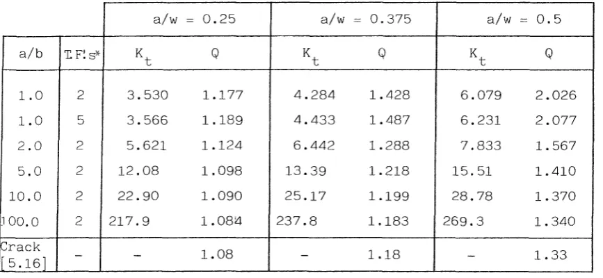
Q parameter defined as K,/K
r radial polar coordinate
R = for an elliptical hole
R ratio of special region area to area of hole
s distance along an element side measured from node (1)
s length of element side
o
5 boundary of region (see above)
t thickness of finite elements in the special region
T tractions (see above)
u displacements (see above)
U strain energy function
Ug Q strain energy function evaluated in the special region
V complete region
w half width of plate
X,Y Cartesian coordinates referred to global axes
x,y Cartesian coordinates referred to trial function axes
z complex number = x + i y
a. coefficient of trial function or, if i=0, of the loading function
a vector of trial function coefficients a (i=l to k) a' vector of coefficients a. (i=0 to k)
— 1
6 half angle subtended by arc of pressure
Y angle between OX and O'x axes
Y shear strain component (see above for qualifiers) 6^ typical linear dimension of elements near hole
A area of triangular element
£ strain vector (see above)
E ^ percentage difference term for comparing two values of maximum stress see equation (5.1) for definition
5 complex function of z
6 angular polar coordinate
8 arbitrary angle
K = (for plane stress)
^ Lagrange multiplier
u = r for an elliptical hole
a+b
V Poisson's ratio
C complex function of z
n pi = 3.1415927
n functional (complementary energy)
n modified functional
c
0
o nominal applied stress 0
max maximum tensile stress 0
com maximum compressive stress ^ref value of stress for comparison
T shear stress component (see above for qualifiers)
* angle between X axis and outward normal to boundary <t>.
1 complex stress function for trial function
*A Airy stress function
*i complex stress function for trial function <=° infinity
Other notation:
log natural logarithm
Im denotes imaginary part of complex number Re denotes real part of complex number
(bar) unless referred to above denotes complex conjugate (prime) 1 unless referred to above denotes
" (double prime)/ differentiation
5{ } denotes the variation of a functional
^ denotes summation
denotes proportional to T
) denotes the transpose of a vector
_ underlined symbols denote vectors or matrices
Notation for PART II (including Appendix F)
In Part II tensor notation is used whereby subscripts - for example i, j or k - denote the direction of components. The following tensor variables are used:
kr body force
cosine of the angle between the boundary normal and i coordinate axis
T. traction
1
u displacement
E.. strain ij
o. . stress
ij
C. position of the point at which the kernel function is evaluated
Tensors referring to the kernel function are denoted by the superscript * and have an additional subscript (before other subscripts) which indicates the direction of the point force.
A subscript preceded by a comma (e.g. u. .) means partial differentiation 1 > J
with respect to the coordinate component x . A repeated suffix implies summation.
The following superscripts may also be used:
K c
m or n P
corresponding to the Kelvin solution
complementary part of the kernel function (added to Kelvin solution yields the kernel function)
pertaining to the m'th or n'th node or element pertaining to an internal point
Boundaries are denoted by S with the following qualifiers:
none complete boundary of the problem n (subscript) n'th boundary element
* (superscript) boundary included in the kernel function H (subscript) part of the boundary of the problem
co-inciding with S*
' (prime) remainder of the boundary of the problem
Other symbols:
a radius of circular hole
b (see above)
A matrix of the coefficients of the unknown tractions or displacements
c coefficient of displacement in Somigliana's identity (6.17). A superscript may denote the coefficient for a particular element.
(italic) function defined by equation (6.32)
f arbitrary function
F vector of right-hand sides in the simultaneous equations 7, coefficient of the tractions defined by equation (6.24)
k&mn
G shear modulus
G matrix of the traction coefficients
h, coefficient of the displacements defined by equations (6.22) and (6.23)
H matrix of the displacement coefficients
1 / T
integers defining coordinate directions K number of dimensions of the problem (2 or 3) K stress concentration factor
L complex number =
& (see above)
m element (or node) number
n node (or element) number
N number of elements and nodes
r radial polar coordinate
S boundary (see above)
(italic) function defined by equation (6.33)
T (see above)
V region of the problem
u (see above)
w radius of annulus or half width of square plate
X (see above)
z complex number defining position of point in plane (= + iCg)
z complex number defining position of the point force
° (= + iXg)
Kronecker delta. See equation (6.5)
6(x-() Dirac delta function. See equations (6.13)-(6.15) (see above)
E percentage difference term for comparing two values of stress. See equation (5.1) for definition
8 angular polar coordinate
K = (for plane stress)
1 + v
= 3-4v (for plane strain)
V Poisson's ratio
X Lame constant given by equation (6.3)
C. (see above)
m pi = 3.1415927
o.. (see above)
ij
o externally applied stress
o , Og radial and tangential components of stress complex number = 5^ +
complex potential for the kernel function with the point for
infinity k
j point force in the k direction
Other notation:
&n natural logarithm
Im denotes imaginary part of complex number Re denotes real part of complex number
(bar) denotes complex conjugate
' (prime) 1 , „ , , ,
\ unless referred to above denotes " (double prime j differentiation with respect to z
I denotes summation
.J (subscript) denotes partial differentiation with respect to X .
J
€ denotes "is included in..."
{ }dV(C) denotes integration over V with respect to the variable 5
LIST OF FIGURES
Figure Page
2.1 Two dimensional body with loaded hole 15
2.2 Two dimensional body showing special region 15
4.1 Structure of the FESM program 43
4.2 Areas of element on hole boundary 44
4.3 Boundary conditions subroutine 47
5.1 Rectangular plate with a central elliptical (or
circular) hole 52
5.2 Effect of mesh refinement on the accuracy of the
stress concentration factor 55
5.3 Effect of hole size on the accuracy of the stress
concentration factor 57
5.4 Effect of hole aspect ratio on the accuracy of the
stress concentration factor 59
5.5 Effect of special region size on accuracy for mesh A 65 5.6 Effect of special region size on accuracy for mesh B 66
5.7 Square plate with circular hole 69
5.8 Stress concentration results for square plate with
elliptical holes of varying aspect ratios 74
5.9 Stress concentration results for square plate with
elliptical holes of varying size 75
5.10 Use of a superposition principle to derive the stress concentration factor for the loaded lug (ii) from the
configuration (i) 78
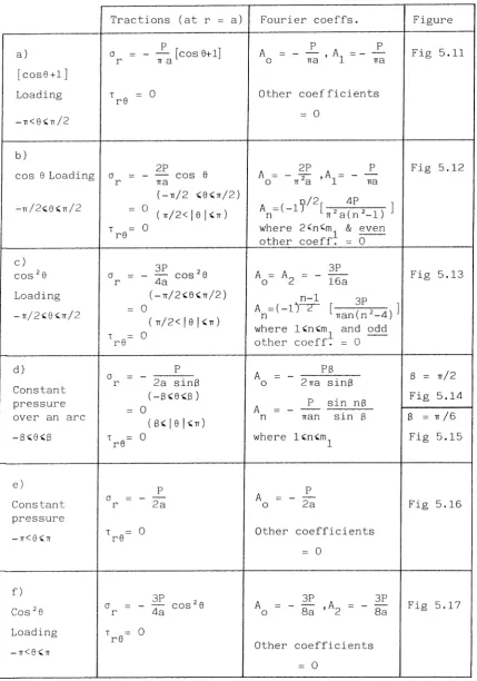
5.11 Stresses around boundary of hole in infinite sheet.
Loading a) Pressure =[cos8+l](-n<8<w) 79
5.12 Stresses around boundary of hole in infinite sheet.
Loading b) Pressure = cos8 (-n/2<8<n/2) 81 5.13 Stresses around boundary of hole in infinite sheet.
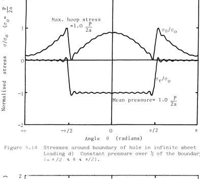
Loading c) Pressure = cos^e (-n/2<8<n/2) 82 5.14 Stresses around boundary of hole in infinite sheet.
Loading d) Constant pressure over % of the boundary
(-n/2<8<m/2) 83
5.15 Stresses around boundary of hole in infinite sheet. Loading d) Constant pressure over 1/6 of the boundary
(-n/6<8<n/6) 83
5.16 Stresses around boundary of hole in infinite sheet.
Loading e) Constant pressure (-n<8<n) 84
5.17 Stresses around boundary of hole in infinite sheet.
Loading f) Pressure = cos*8 (-w<8<n) 85
5.18 Stresses around boundary of hole in infinite sheet.
Figure Page 5.19 Stresses around boundary of hole in infinite sheet.
ii) Loading b) + h) cosG normal pressure & sin28 shear 88 5.20 Stresses around boundary of hole in infinite sheet.
iii) Loading b) + j) cos8 normal pressure & sin^GcosG 88 shear
5.21 Stresses around boundary of hole in infinite sheet.
iv) Loading c) + g) cos*8normal pressure & sine shear 90 5.22 Stresses around boundary of hole in infinite sheet.
v) Loading c) + h) cos*8normal pressure & sin8 shear 90 5.23 Stresses around boundary of hole in infinite sheet.
vi) Loading c) + j) cos^Snormal pressure & sin^G cos8 91 shear
5.24 Pressurized annulus 92
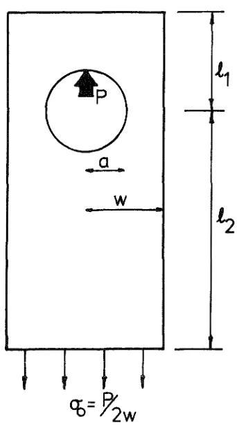
5.25 Symmetrical lug (pin-loaded) 94
5.26 Rectangular lug (pin-loaded) 98
5.27 Stress concentration factors for symmetrical/
asymmetrical loaded lugs 100
5.28 Stress concentration factors for loaded lugs 101
5.29 Lug with rounded end 103
5.30 Comparison of stress concentration factors for
rectangular lugs (FESM) with rounded lugs 103
6.1 Boundaries with modified kernel function 115
7.1 Externally loaded annulus 119
7.2 Square plate with central circular hole in biaxial
tension 120
7.3 Comparison of results for in externally loaded
annulus 121
7.4 Comparison of results for o in externally loaded
annulus 123
7.5 Accuracy of the modified BEM solution for annuli with
various sizes of hole 124
7.6 Accuracy of the modified BEM solution for square plates
with various sizes of hole 126
(Appendices)
E1-E29 Finite element meshes 197
LIST OF TABLES
Table Page
5.1 The stress concentration factor for rectangular plate
in tension (a/w = 0.5) for different meshes 54
5.2 The stress concentration factor for rectangular plate
in tension with various sizes of circular hole 56
5.3 The stress concentration factor for rectangular plate in tension with elliptical hole of varying aspect ratio
(a/w = 0.25) 58
5.4 The stress concentration factor for rectangular plate in tension with elliptical hole of varying aspect ratio
(a/w = 0.5) 58
5.5 Reference values of stress at the edge of a circular
hole in an infinite strip in tension (a/w = 0.5) 61
5.6 The stress concentration factors for different special
regions. Mesh A. 62
5.7 The stress concentration factors for different special
regions. Mesh B. 63
5.8 Stress concentration factors for plate with circular hole (a/w = 0.5) using different finite element meshes 68
5.9 Stress concentration factors given by reference [5.5]
for square plate in tension with circular hole. 70
5.10 Stress concentration factors for square plate with
circular hole (a/w = 0.5) by FESM 71
5.11 Stress concentration factors for square plate with
circular hole (a/w = 0.5) by other finite element methods 71
5.12 Stress concentration factors for square plate in tension
with elliptical hole 73
5.13 Tractions and Fourier coefficients for various
distributions of radial load 80
5.14 Tractions and Fourier coefficients for various
distributions of shear 86
5.15 Results for pressurized hole 93
5.16 Stress concentrations for symmetrical lug with different
distributions of load 95
5.17 Stress concentration factor for rectangular pin-loaded
lugs 99
5.18 Stress concentration factors for a lug with rounded
Table Page
(Appendices)
B.l Programs segments listed in this appendix (B) 157
B.2 Other program segments used by FESM program 158
C.l Information stored in the direct access file 179
C.2 Variables in the direct access file 180
CHAPTER 1
GENERAL INTRODUCTION
1.1 Background to the work
The presence of holes or notches in structural components increases the nominal stress in these components by a factor, K^, known as the stress concentration factor [l.l]. The aim of this work has been the development of acc
wide variety of configurations,
has been the development of accurate methods for determining in a
The need for accurate estimates of stress concentration factors has arisen in particular from studies in fracture mechanics. Fatigue damage may be caused by the initiation and growth of cracks near stress concentrations when the structure is subject to cyclic loading. Since these cracks may appear early in the rLfe of 1±e structure, or indeed may occur in manufacture, the fatigue life depends on the rate at which the crack grows, and to determine crack growth rates the stress
factor for the crack must be known. Stress factors characterise the stress field near to a crack tip and values for most simple config-urations have been collected in reference manuals [1.2-1.4], For short cracks - and for most of the life of a component the crack will be short-simple methods of determining the stress factor [1.5,1.6] may be used even for complex geometries, provided that data is available for the stress concentration factor or, in the case of weight function
methods, the stress distribution over the crack site in the absence of the crack. The recent compounding method for determining stress
factors [1.7-1.9] also requires knowledge of the stress concentration factor at the site of the crack if there is significant interaction between the boundaries of the configuration [1.10], (e.g. when the hole is close to the edge of the component). Furthermore since the crack growth rate depends on the stress factor raised to a power
included. Hence there is a need for an accurate, versatile and convenient method for determining stress concentration factors and the stress distribution near to holes and notches.
For methods to be applicable to a variety of complex structures with several interacting boundaries and varied loading conditions, a numerical method of stress analysis is required. Broadly these may be divided into three main types: finite difference methods, finite element methods and boundary element methods. The finite difference method is perhaps the most straight forward and historically was developed first
[l.ll]. By dividing the region of the problem with equally spaced nodes throughout ,the governing differential equation may be solved in terms of values of stress or displacement at the nodal points. However the
method is not suited to problems where there are high stress gradients,
such as occur at holes or notches, since the nodes must be closely spaced to model the region of stress concentration, and consequently the total number required for an accurate representation of the solution becomes very large. For this reason finite difference methods have been largely superseded by finite elements [1.12-1.13] for all but specialized
applications, and the two methods developed in the present work are based on the finite element and boundary element methods.
The finite element method is widely used in all branches of continuum mechanics and since its inception for stress analysis [1.14] it has been developed to include many variants. The basis of the method is that the region of the problem is divided into small elements of simple shape (in two dimensions usually triangles or quadrilaterals) which are assumed to be interconnected only at a discrete number of nodes. A "shape function", for example a polynomial, is used to represent the stresses or displacements within the elements in terms of the nodal values of either displacements, stresses or both, depending on the particular formulation. An approximate solution for these nodal unknowns is obtained by applying a weighted residual technique or variational principle (for example minimizing energy) to give a set of symmetric banded simultaneous equations [1.15, 1.16]. The technique is extremely powerful and has been applied successfully to many different problems including three-dimensional, anisotropic and non-linear cases.
-Some of the considerable amount of work done with finite elements for two dimensional elastic problems with high stress gradients is reviewed, along with other methods, in section 1.2. In developing a new method for stress concentrations near holes, as described in Part I of this work, certain drawbacks of the finite element method are avoided. Firstly in areas of steep stress gradient, such as found at stress concentrations, the finite element method usually requires a very fine mesh to obtain acceptable accuracy. This is expensive in both data preparation time and run time on the computer. Furthermore the simplest finite element methods used constant strain triangular elements with nodal displacements as unknowns. This means that to estimate the stress at any boundary {the edge of a hole for example) the value must be extrapolated from the average stress in the elements near to the boundary, introducing a further source of error. By incorporating into the finite element scheme known elasticity solutions, such as that for an infinite sheet with a hole, the new method proposed and developed in this thesis increases the effectiveness of finite elements for stress concentration problems.
this enables this part of the boundary to be included without using boundary elements. Thus the required stresses may be determined as accurately as at interior points and the number of elements needed is reduced.
1.2 Review of theoretical methods and solutions
The existence of high stress near geometrical discontinuities has been appreciated for many years and investigations of stress concen-trations, both experimental and theoretical, were begun during the last century [1.19-1.21]. Since that time an immense volume of work has been published on the subject and this review is aimed at highlighting some of the more important work. Reviews of general methods of obtaining stress concentrations [1.22] and of analytical methods in particular,
[1.23, 1.24] have appeared in the literature and several collections of the solutions obtained have been made [l.l, 1.25-1.31] . The aim of the present survey is to consider the various theoretical methods available for obtaining stress concentration factors and to compare them with the finite element superposition method (FESM) and the modified boundary element method (BEM) which are developed in Parts I and II respectively. The review is limited to methods applied to two d'trngMStOMoI configurations of elastic, isotropic and homogeneous materials with in-plane loadings. An assessment is made of the relative merits of the methods, the accuracy
(where known), whether the methods may be extended to more complex
geometries or materials (e.g. three-dimensional configurations, anisotropic materials, etc.) and, in general terms, their theoretical basis.
1.2.1 Exact Analytical Methods
The solution by Lame [1.19] to the case of a hollow cylinder subjected to uniform pressure on the inner and outer surfaces, was the precursor of many of the analytical solutions to stress concentration problems. It was based on the mathematical theory of elasticity which was formulated, in a systematic way, during the first part of the last century by Navier [1.32], Cauchy [1.33] and others. The introduction by Airy [1.34] of a formulation using stress functions led to important solutions, including those for an infinite sheet in tension containing a traction-free circular hole [1.20], a traction-free elliptical hole
potentials and conformal mapping. This led to the development of a most powerful analytical method for elasticity problems and much more work was done using this approach by the Russian school, notably Muskhelishvili [l.38-1.40] and co-workers. The technique remained unknown outside Russia for many years and was later used independently by Stevenson [l.41, 1.42] and others [1.43, 1.44] for stress concentration problems. Examples of other solutions obtained using Muskhelishvili's method are: infinite or semi-infinite plates in tension containing deep hyperbolic or shallow semi-elliptical notches [l.3l], and point forces acting in an infinite plate containing a circular [1.45] or elliptical [1.46] cut-out. In spite of the powerful nature of the method and the usefulness of the solutions so obtained, only a ^2w configurations have been solved in closed form, and general solutions not in closed form
(e.g. [1.47]) require much analysis to obtain a particular solution,
even assuming that the series involved converge. For this reason approximate methods for calculating the stresses have been developed and applied to a much wider range of problems than is possible using an exact analytical technique. However the exact methods are most
important in the development of approximate techniques and in the present work exact analytical solutions based on the methods of Airy [1.34] or Muskhelishvili [1.38] are incorporated into numerical methods to improve their efficiency.
1.2.2 Approximate Analytical Methods
Approximate methods such as the "alternating technique" have been used to determine Airy stress functions from a series representation, and hence to obtain the stress in, for example, an infinite strip with
Isida [1.59-1.65] solved several strip configurations using a "perturbation" method based on the alternating technique used by Howland. the solutions included those for strips containing an eccentric circular hole [1.59,1.61], elliptical hole [1.62, 1.63] and symmetrical notches [l.60]. The solution by Shibuya et al [1.66] for a plate with a conical hole is based on a similar principle but extended to 3 dimensions by using a least-squares approximation to satisfy the boundary conditions.
Approximate solutions for plates with different shaped holes have also been obtained based on Muskhelishvili's complex variable approach with conformal mapping. Many variants of the method exist, but generally the hole or notch is mapped on to a unit circle, the complex potentials are determined from the boundary conditions, usually in a series form, and truncation of the series yields an approximate solution. Savin
[1.26, 1.27] and many other authors have obtained solutions for plates perforated by circular holes [1.67-1.69], square, rectangular or
triangular holes [1.70-1.74], reinforced holes [1.75-1.77] and multiple holes [1.78-1.80], and many of these solutions are collected in the two monographs [1.26, 1.27] where many anisotropic and elastic/plastic problems are also treated. The same approach has also been used for some edge notch problems [1.81-1.83].
Results from these approximate analytical methods are generally accurate to within 2% but each problem must be formulated individually and particular mapping functions must be found for each configuration. This may not be possible especially if there are discontinuities in the curvature of the notch. Often there are problems of convergence also, such that an appreciable improvement of accuracy can only be achieved by including a great many more terms in the series representation of the potentials, and this is particularly true when the configurations are of finite size, rather than infinite planes or strips. The
1.2.3 Numerical Methods
The advent of powerful digital computers meant that the emphasis in stress analysis moved from analytical methods to numerical methods. Of these, mention has already been made of the finite difference, finite element and boundary element methods. The "collocation method" however is another important technique.
The collocation method [1.84] consists of using stress functions or complex potentials in series form, the coefficients of the series being unknown. The series are truncated and the coefficients determined by matching the boundary conditions at a finite number of points on the boundary. Hooke [1.85, 1.86] used this method for two-dimensional and a^isymmetric three-dimensional notch problems under tension and bending loads.
The collocation method has been combined with conformal mapping by Bowie and others [1.87, 1.88] and further improved by partitioning the region of the problem into separate sub-regions [1.89]. Solutions for various shapes of edge notches in semi-infinite plates and holes in infinite plates have been obtained using this method [1.90]. The
collocation method may also be combined with other numerical techniques, such as the finite element method [l.9l], which gives added flexibility in its use. Typical accuracy for the method is generally in the region of 1% [1.92] but problems with convergence, ill-conditioning or
sensitivity to the number and distribution of the boundary points may increase the error. Consequently the collocation method is not as
versatile as some other numerical methods and it has received relatively little attention compared to finite or boundary elements. Some work is continuing on the collocation method for the evaluation of stress intensity factors, at the University of Southampton [1.93|.
General reviews of work in finite elements have been presented, for example, in several of the standard texts [1.12, 1.13, 1.94]. Here, however, having mentioned some of the problems of conventional finite elements, particular attention is paid to the development of methods combining both finite element and continuum concepts, of which the finite element superposition method formulated in the present work is an example.
In applying conventional finite element methods to configurations with steep stress gradients, several difficulties occur. Many elements are required to model the stress field accurately and consequently it is expensive for data preparation, computer processing and post-processing of the results. In addition to obtain a value of stress at the boundary some sort of interpolation from interior points may be required. Even higher order elements are not always an advantage since although the number of elements would be reduced (or the accuracy increased) more nodes are introduced per element and this may lead to a similar number of unknowns in the problem. Much work has been done in proposing modifications to the finite element scheme to overcome these problems, particularly for crack problems [1.95]. Isoparametric elements [1.96], different variational principles [1.97], and hybrid methods [1.98]
have all been used to improve the method for cracked configurations. The forerunners of the present work, also using methods formulated for crack problems, superimposed analytical trial functions, corresponding to the singular stress field around a crack tip, over a region of the configuration. This region varied from a special crack-tip element [1.99-1.103] to the whole region of the problem [1.104-1.108] or, as in the present formulation, a "special region" including several elements around the notch or crack [1.109-1.111]. A superposition approach was proposed for stress concentrations at smooth cut-outs by Rao [1.103]
using large "primary" elements in the region of the notch,and by Schnack [1.111] who combined the use of augmenting functions with six-node hybrid elements. The aim of these methods is to incorporate known solutions for the stress field near to a crack or notch in an region, into the finite element scheme. Thus the finite elements model only the
difference between the infinite region solution, scaled by arbitrary
Since this difference will be relatively small in the region of interest if the trial functions are appropriate to the particular problem, the errors introduced by modelling the region with a coarse finite element mesh and interpolating values of stress on the boundary, will also be small.
The finite element superposition method presented in Part I is a development of this work in that trial functions, derived from known elasticity solutions to appropriate configurations, are combined with constant strain triangular finite elements. Loading on a hole boundary is incorporated into the method using similar elasticity solutions, known as loading functions, which remove the need to represent loadings as a series of nodal forces - often a further source of error in
conventional finite element analysis. The trial functions for config-urations with circular holes are based on the general Airy stress
functions, rather than solutions for infinite regions, which means that the effects of the other parts of the boundary may also be included in the trial functions to some extent. The accuracy and small number of degrees of freedom that result from well chosen trial and loading
functions, and the versatility of the finite element method in general combine to make this a powerful method for the solution of stress concentration problems.
The boundary element method was proposed not long after the finite element method, but the first practical applications of the method by Jaswon and Symm [1.112, 1.113] appeared in 1963 and initial development was much less rapid than finite elements. This may possibly be due to the slightly greater mathematical complexity of the formulation, and the fact that it is less easily understood intuitively. However the method has several advantages over finite elements, the most important being that since only the boundary of the region need be divided into elements the dimensions of the elements are reduced by one, e.g. from a three-dimensional volume to a two three-dimensional surface. The method was first used for elastostatic problems by Cruse and Rizzo [1.114, 1.115] and in recent years an upsurge in interest in the method has taken place due to its claimed superiority over the finite element method for many
in the boundary integral equations are the physical variables of the problem (e.g. tractions and displacements), and indirect formulations
[1.122-1.125] in which the integral equations are expressed in terms of a "density function", which in itself has no physical significance but from which the physical parameters may be derived at any point in the body. A form of indirect method, called the "body force method" developed by Nisitani [1.126] has been used for many notch and crack problems [1.46, 1.127-1.129] . These include an infinite sheet
containing one or two rows of elliptical holes, a semi-infinite plate containing variously shaped notches, a row of elliptical holes or a row of notches, and an infinite strip containing two symmetrical semi-elliptical notches.
Much of the recent interest in boundary elements, as with finite elements, centred on improving the method for configurations with cracks. Cruse [1.130] proposed including the crack explicitly in the fundamental solution from which the integral equations are derived so that the crack need not be modelled by boundary elements, and this proved most successful. In the case of the body force method a similar approach was adopted by Murakami and Nisitani for elliptical holes
[1.131, 1.132] and, using a direct boundary element method, Telles and Brebbia [1.133-1.134] used the approach for configurations containing a long straight boundary. The success of these methods suggested that a similar approach could be used for a direct boundary element
formulation with a fundamental solution which satisfied the boundary conditions of a circular hole. This idea is the basis of the work
1. 3 Layout of the thesis
The main body of the thesis is divided into two parts: Part I comprising Chapters 2 to 5 is concerned with the work on finite elements and Part II comprising Chapters 6 and 7 concerns the boundary element work. Chapters 1 and 8 are general to both aspects of the work.
CHAPTER 2 presents the formulation of the finite element super-position method. The concept of trial functions derived from known elasticity solutions is introduced for configurations with loaded or traction-free holes. In addition to the trial functions the new loading function is incorporated into the method which is the (known) solution for an infinite sheet with the specified loading on the hole. A
variational principle is used to determine the arbitrary coefficients of the trial functions, the finite element unknowns (nodal displace-ments) and certain correction stresses which arise in elements near boundaries.
CHAPTER 3 deals with the analytical elasticity solutions which are required by the finite element superposition method, i.e. the trial functions and loading function. Two trial functions are given for elliptical holes based on an analytical solution using complex stress functions and a conformal mapping function. For circular holes the generalised solution for the Airy stress function in two dimensional polar coordinates is used to specify a general set of trial functions. The generalised solution is also used to give the loading function, with a distribution of tractions round the hole boundary specified using a Fourier expansion.
In CHAPTER 4 the way in which the method is implemented on the computer is explained. The structure and the main processes occurring in the program are discussed and a brief resume is given of how the program and its peripheral facilities may be used in practice.
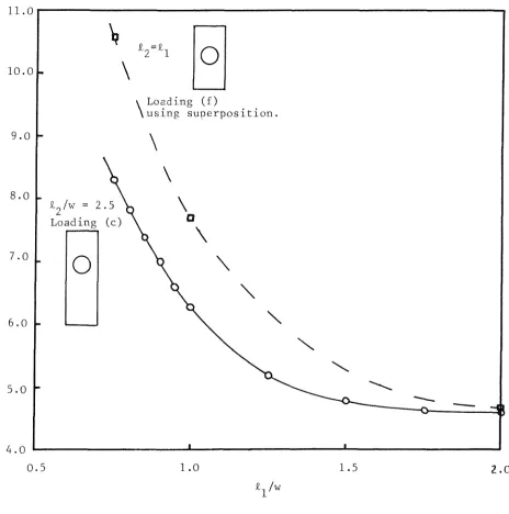
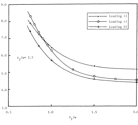
effect on accuracy of such parameters as the finite element mesh size, number of trial functions and size of the hole is determined and new results for the stress concentration factors of elliptical traction-free holes in square plates are given. Various distributions for the tractions on loaded holes are suggested and compared. Estimates for stress concentration factors for loaded holes determined by the finite element superposition method are compared with some known values and finally new results are obtained for rectangular lugs wilWh loaded holes.
In CHAPTER 6 the formulation of the boundary element method is presented and the modification to the method, by using fundamental solutions which include the boundary near the stress concentration, is explained. The implementation of these modifications in the computer program is also discussed.
The results given in CHAPTER 7 were obtained using the modified boundary element method. The advantages and limitations of the modified method are shown by comparing the results from the two methods for an externally pressurized annulus. The accuracy of the modified method for annuli and square plates with various sizes of circular hole is shown by comparing the estimates for stress concentration factors from the boundary element program with known values.
CHAPTER 8, the final chapter, contains a summary of the conclusions from both the finite element and boundary element work. Comparison
P A R T I
CHAPTER 2
FINITE ELEMENT FORMULATION
2.1 Introduction
The finite element superposition method (FESM) used in this work is based on a method originated by Morley [2.l] and extended by
Bartholomew [2.2, 2.3]. basis of the method is that Wie piece-wise linear displacement field of constant strain finite elements may be
augmented by the superposition of one or more known elasticity solutions, referred to as the "trial functions", which are weighted by arbitrary coefficients.* The trial functions are elasticity solutions which satisfy exactly conditions of equilibrium and compatibility but not all the boundary conditions of the problem. They are chosen such that they give rise to stresses and displacements closely matching those in the region of the stress concentration. For example the known solution for a uniformly stressed infinite sheet containing a circular hole may be used as a trial function for a finite plate loaded in some manner with a similar hole.
Bartholomew has formulated this method for traction-free cracks. In the present work the method is extended to apply to configurations with circular or elliptical holes which may be traction-free or subjected to specified tractions. To deal with loaded holes another known elasticity solution referred to as the "loading function" has been introduced. The use of this function removes the need to represent the tractions at the hole in the piece-wise constant form usually employed by the finite element method, thus avoiding the introduction of
inaccuracies at the very point where the stress concentration factor is to be determined.
The loading function corresponds to the elasticity solution in which the hole is subjected to the tractions for which a solution is
required but the extent of the sheet is assumed to be infinite. The trial functions, on the other hand, are elasticity solutions for a plate with a stress-yreg hole under various different remote boundary conditions which need not necessarily correspond to an infinite region. The superposition of the loading function and these trial functions therefore, results in the traction boundary conditions on the hole being satisfied exactly and leaves residuals remote from the l^3le which are corrected by the constant strain finite elements.
It has been shown [2.3] that in the case of cracked configurations it is advantageous to limit the superposition to a "special region" which is larger than a single special element but smaller than the
complete region of the problem. For this reason the present formulation continues the use of a special region over which the trial functions and loading function are superimposed, constant strain elements alone being used in the exterior region.
The trial functions and loading function for specific classes of problem are determined in Chapter 3. The details of how the method is formulated are outlined in the remainder of this chapter, with additional material in Appendix A.
2.2 Notation for the boundaries
The configuration to be analysed by FESM may be represented diagramatically as in figure 2.1. The two dimensional body containing a hole is denoted V and the boundary, including the hole boundary, is denoted by S. The boundary S is made up of S , where traction boundary conditions are applied, and S , where kinematic boundary conditions are applied. Since a superposition principle is to be used in the represent-ation of load on the hole boundary, it is assumed that the hole forms part of S . The geometry of the configuration is defined relative to Cartesian coordinates (X,Y) with an origin at 0.
The variational principle, from which the finite element solution is derived, will be represented in terms of volume and boundary integrals
Y
0
Loaded hole
©
Applied Tractions (T)
Prescribed
displacement
(u)
X
Figure 2.1 Two dimensional body with loaded hole
Exterior region
O
Special Region
(Sp.R)
Boundaries adjacent to the special region are denoted with a prime ('), hence for example. The traction boundary adjacent to the special region is divided into two parts, the hole boundary and the remaining traction boundaries. This distinction is necessary in the present work due to the introduction of the loading function to represent the loading on the hole. The "interface boundary" between the special region and exterior region is denoted S^. The notation for the
boundaries may be summarized therefore as follows:
and
S = 5% + S,
S'
^T =
( 2 . 1 )
where S denotes that part of the traction boundary in the exterior region. The complete region V is divided into triangular elements.
2.3 Displacement and stress fields
The basis of FESM is that the displacements, u , and stresses,
I
a , of the approximate solution are a superposition of a constant strain finite element field and a set of known elasticity solutions with
dis-* *
placements and stresses denoted u and j respectively. The integer i takes the values 1 to k for the trial functions, k being the number of trial functions, and i=0 for the loading function. (Underlined symbols are used throughout the text to define both vector fields and matrices).
The assumed form of the displacement field u on the boundaries of the finite elements may therefore be expressed as follows:
k I i=0
u = u" + J a. (u. - u^;
— — —1 —1
within the special region, on and
in the external region, on and
> ( 2 . 2 )
where a. is the coefficient of the i'th trial function, 1
u
and t
are the prescribed displacements on S ,
u are constant strain finite element fields which take the *
same values as u. at the finite element nodes and are linear between
-1 t
nodes. The reason for introducing these fields, u., is that (u. - u.)
—1 —1 —1
is zero at the nodes thus nodal displacements are given simply by p
u in both the exterior and special regions and the displacement field, as defined by equation (2.2) is compatible across all element boundaries.
As is usual in the development of finite element methods the
piece-F t
wise linear displacement fields u and u. ;&re expressed in terms of
F t - -1
vectors, q and q. respectively, containing the components of displace-ment at the nodes. The strain within an eledisplace-ment is constant from these fields and thus may be expressed in terms of the nodal displacements as:
and
-N %
1 -N. 1
(2.3)
F
where q' and q_, contain displacement components for the N'th element
—N —
only, B is the "element strain matrix" and and are the cons tant strain vectors (three components in plane stress} for the respective fields. The matrix is obtained from the geometry of the element and is given ; as in reference [2.4], by:
-^il)' ^^2)' -(3) (2.4)
where a typical sub-matrix, say, is:
:i) 2 A
' V s '
(X3-X2)
(X3-X^) (2.5)
and A is the area of the element, X , Y are the coordinates of the n n
The stress field o may now be defined in the intertor of each element as follows:
I F r + T 4 - k - 1
-0 = a + ^ a. (o. - a. + o. J In the special region
i=0 1 ^ 1 ^
I F
a = a In the external region.
( 2 . 6 )
F * t
The stress fields a , 0. and a. correspond to exact solutions for
^ F * ^ t c
the displacement fields u , u. and u. respectively. The terms a.
— —1 —1 —1
constant within elements, must be included in the special region due to linear displacements being defined on the boundaries and to ensure compatibility. The terms therefore are non-zero only in special region elements adjacent to kinematic or interface boundaries. In spite of the many terms in equation (2.6a) it may be seen that it is
F t
simply the superposition of constant finite element fields, a , 0.
c * "
and a. , with the trial function fields 0. .
—1 —1
Again following standard finite element methods, the constant stress fields for an element may be expressed in terms of strain. Thus:
and
A 0 N
t -N.
1
A 0 N.
1
-N. 1
-N. 1
(2.7)
, F t c F t
where 0^ , , contain the stress and
strain components respectively for the^N'th element, and
1
E —v 0
1 0
0 2(l+v) ( 2 . 8 )
In order to determine displacements and stresses from the F
equations (2.2) and (2.6), the nodal displacements, q , the trial function coefficients, a., and the correction stress fields, o? ,
1 —1
must be known. These are determined using a variational principle.
2.4 The variational principle
A variational principle uses a scalar quantity (a "functional") which may be defined in terms of integrals of the unknown parameters in a continuum problem - in this case displacement and stress. The functions of the parameters which make the functional stationary is the solution to the problem. By limiting the possible functions of displacement and stress to a set of trial functions (as above) with finite degrees of freedom the problem may be reduced to a set of simultaneous equations.
The specification of both displacements and stresses by equations (2.2) and (2.6) means that the variational principle must allow for trial functions to be specified for both parameters. Such a variational principle derived from a modified principle of minimum complementary energy (see Appendix A) was given by Pian and Tong [2.5]: .
n = I { (o^) + I c (u)^ dS - I (u)T f dS } (2.9)
N N - J - - Js^ -
-where U (j^) is the strain energy of the specified field for the N'th
T I
element, a and T are respectively the interior stress and corresponding tractions for the element, u is the displacement on the complete element boundary, which is denoted by S , and T are the prescribed tractions
' T
on the element traction boundary S . The superscript ( ) denotes the N
the transpose of a vector of matrix. The summation is carried out over all the elements.
In general the function U(o ,02) is defined as the strain energy, in the region V bounded by the surface S, due to two stress fields G_
— 1 and On . Thus:
—
1 [ , - T -1^ ^2 V
^ 2 ' Og) = 2 J dV ( 2 . 1 0 )
If only one parameter is specified to the function the two fields in equation (2.10) are understood to be the same. Similarly the function may be written with displacement rather than stress fields as the variables. Provided that for one field, o say, the stresses are in equilibrium over V and for the other the strain field is compatible over V, the volume integral may be reduced to a surface integral using the divergence theorem:
1 f sT
" 2 S
U(o^,a^) = - j (T^) dS (2.11)
where T_, and u„ are the tractions and displacements respectively of
—1 —ri
the two fields and there are no body forces. Using these properties of the strain energy function and substituting equations (2.2) and (2.6) into equation (2.9) the following form of the functional is obtained;
F F T
-n = U(u ) - I (u ) T dS
C - Jo ~
T
k I
i=0 ^ L I ^ - J s > s . 'h*- '"T "H I
1 ^ ^ f * t T *
- I I a. a. I (u. - 2uT) T. dS " lio jio ' J 's'.s'
^ F T * '' * + T F
I (u) T. dS + I (u ) T. dS - I (u.-LL^ T dS
^ ^ I f * T * r * + T +
+ f f a.o. [ - % I (u.) T. dS + I (u.-u.l T? dS
1 = 0 j ' o ^ J ' 2 - 1 - J - 1 - 1 - J
( u * - T": d S I ( 2 . 1 2 )
where with the appropriate subscripts and superscripts, denotes the
The prescribed tractions on the hole boundary are applied explicitly using the loading function. This function is defined such that:
= f (on the hole boundary S') (2.13)
0 —0 — H
Since a , the coefficient of the loading function, is constant it is not a trial function. It is included in the functional with the trial functions but the coefficient is determined by the magnitude of the loading on the hole and thus it does not appear as an unknown in the final system of equations.
The trial functions are chosen to satisfy zero traction conditions on the hole boundary, i.e.:
T. = 0 (on S', for i=l to k) (2.14)
—1 H
By substituting equation (2.13) in the functional, equation (2.12), the terms which relate to the traction boundaries may be rewritten as:
r p T — f F T * f f T T S
-- I (u ) T dS - On I (u ) T_ dS + a_ I (u ) T dS
- - 0 Jc, - 0 0 Jc, - -0
% a. [ (u^)^^ T* dS + % a. [I (u^)^ T* - f I dS]
^ f k k ^
I Go*i I (Hi-Hi) lo dS + I I OiO. j (Hi-Hi) I. dS
i=0 ^ i=0 j=0 1 J J
^ ^ f * + T * -I r * T *
f % a.a. [ I (u. - ul) T. dS - - I (u.) T. dS ] (2.15)
iio j i o ' J
Js'
'
-J
2
-J
"c ' " ° i % . H * J o j o •"sp.R'aI-^]'-%.H'2l'Hr
f F T - ^ f F T * I" * t T
-- I (u ) T dS + I a. [I (u ) T. - | (u.-u.) T dS
i=o 1 1 1 1
^ ^ r * f T * 1 f * T *
+ % X a.a. [I (u.-u.) T. dS - - I (u.) T. dS]
i'o jlo ' : 's- -J : 's' -J
+
^ r _ ' r * r f
% a. [| (u) T. dS + (u ) T. dS - (u.-u.) T dS]
.=0 ' i s - - J s . " -
-y ^ r * + T r * + T r
+ 2 X a.a. [ I (u.-u.) T. dS - I (u.-u.) T. dS
i=0 j=0 1 J ^ ^ ^ ^ ^ J
(2.16)
2.5 Determination of the correction stress fields a? —1
The correction stress fields are determined by variation of the functional equation (2.16), with respect to The terms which depend
c on a. are:
—1
I I ( , ^ o 5 ) - I (h'-HI)' 1= dS I (2.17)
- j-u
Since the stresses 2^ are constant over each element, the expression (2.17) may be expressed:
( S p . R ) ^ ^
1 , , C\T . c , c/r a a [
-N i=0 j=0
I { I I a.Oj [- ^ t A(o^^l' A 2^^ - (o^])^ L C^] } (2.18)
where the summation is carried out over all elements in the special region, t is the thickness of the elements in the special region and
is the vector of components of the correction stress field in the —Ni
Thus:
-Ni o
o, Xi
c Yi c
(2.19)
T . being the shear component. L is the matrix which when
pre-XYi ^ ^
multiplied by the vector ( o ^ ) gives the tractions on the part of the boundary adjacent to the element, i.e.
cos *
0
sin $
0 sin
cos : 2 . 2 0 )
where $ is the angle between the X axis and the normal to the boundary. Finally is defined by:
C.
—1 Xi
Yi
Xi'
- u Yi'
dS
dS (2.21)
when the subscript N denotes the part of the boundary of the N'th element and the suffices X and Y denote the components in the X and Y coordinate directions respectively. At the stationary point the variation
c
of (2.18) with respect to the variables (i = 0 to k, N = 1 to the number of elements in the special region) is zero. Thus the components of 0-^ may be determined, in terms of integrals of the known fields
* ^ j
-u and , by differentiating equation (2.18). They are given by:
-Ni tA L C. :2.22)
where A IS;
V
0
V
1 0
2 0 0
(1- (2.23)
F 2.6 Determination of the nodal displacements q
The constant strain finite element part of the displacement field,
F F
u , is defined by the vector q of its nodal components. The terms in
" F
equation (2.16) which depend on u are as follows:
F C F T - r F T *
U(u ) - I (u ) T dS + I a. { I (u ) T. dS
r * t T F F t
(u. - u.) T dS - 2 U_ a (u ,U.) } (2.24)
c,,q, -1 -1 - Sp.R - -1
F
In terms of q this may be written;
i (gF)T K qF _ (gF)T & + f o (qf)? p (2.25) i=0
where K is the stiffness matrix for the constant strain finite element scheme and p and p. are vectors which may be considered as equivalent
— —1
nodal loads. K is assembled from the stiffness matrices of individual elements as for conventional finite element methods. Thus the first term of equation (2.24) may be written:
I tA(c;)? A-l c? (2.26)
N
I t6(c|F)T [ ] gF (2.27)
where the summation is over all elements. The element stiffness matrix therefore is given by tA [B^ A ^ B^] and by summing the contributions from each element the stiffness matrix K is obtained.
The vector p is determined simply from the prescribed tractions T (excluding the tractions on the hole boundary A uniform load on an element traction boundary is distributed equally between the 2 nodes on the element side.
Contributions to the vector p. however arise from the last three —1
terms in expression (2.24). From the first of these terms the following equivalent nodal loads arise in an element with a part of the boundary
:2)
f ( 2 )
t I (1
^ ( 1 )
- - ) T. dS
s — 1
o
- i T- dS
:i) ^
> on or
( 2 . 2 8 )
where s is the distance along the element side measured from node (1),
is the length of the element side and the suffix to pj ^ denotes
the node at which the equivalent load is considered to act. The integral
is of a known function and may be carried out numerically. The remaining
two terms of equation (2.24) may be written:
Sp. R
C.
—1
tA
-Ni * (2.29)
where the summation is carried out for elements in the special region and
"t" t
the vector contains the components of o. for the N'th element.
-Ni -1
The expression (2.29) may be rearranged, using equation (2.22) and the
definition of the matrix (equations (2.3) to (2.5)), as:
SP'R c t T F
I t - tA (o^i + ENi) SN } (2.30)
Thus the contributions to the nodal loads p. in the N'th element from —1
these terms are given by:
and (2.31)
which may be evaluated when the stresses and are calculated
for each element in the special region.
Since the matrices 2 ^^d p in the expression (2.25) can be
determined, the stationary point may be found by setting the variation F
of the expression with respect to q as zero, thus:
K q
i =0 Ei
The variables q and q. are now defined such that:
— —1
q = p (2.33)
and q. = K ^ p. (2.34)
These simultaneous equations, subject to the kinematic constraints
on 5%,
and q. = 0 J (2.35)
—1
are solved on the computer using Choleski factorisation of the matrix in banded form, as implemented by Morley [2.6] and others [2.7, 2.8]. The displacements g, as defined by equations (2.33) are those which would arise from constant strain finite elements if no augmenting trial functions were used. This "basic" solution may be used for comparison in assessing the improvement in the final augmented solution.
F
The nodal displacements, q , written in terms of q and q follow from equations (2.32) to (2.34) and are given by:
q^ = q - % a q. (2.36)
i=0 ^
2.7 Determination of the trial function coefficients
Equation (2.36) may be substituted back into equation (2.25) and hence into the functional, equation (2.16). Furthermore the following terms from equation (2.16) may also be combined:
J o J o "i-j' "sp.n'Hl.Mjl - "sp.R'Hi, M])
f * + T t f * t T r
+ I (u.-u.) T. dS - I (u.-u.) T. dS } (2.37)
1" c
Since the stresses o. and o' are constant over each element the final
—1 —1