Linguistic categorization and complexity

Linguistic categorization and complexity

Katya Pertsova UNC-Chapel Hill Linguistics Dept, CB 3155 Chapel Hill, NC 27599, USA

[email protected]

Abstract

This paper presents a memoryless categoriza-tion learner that predicts differences in cate-gory complexity found in several psycholin-guistic and psychological experiments. In par-ticular, this learner predicts the order of diffi-culty of learning simple Boolean categories, including the advantage of conjunctive cate-gories over the disjunctive ones (an advantage that is not typically modeled by the statistical approaches). It also models the effect of la-beling (positive and negative labels vs. posi-tive labels of two different kinds) on category complexity. This effect has implications for the differences between learning a single cat-egory (e.g., a phonological class of segments) vs. a set of non-overlapping categories (e.g., affixes in a morphological paradigm).

1 Introduction

Learning a linguistic structure typically involves cat-egorization. By “categorization” I mean the task of dividing the data into subsets, as in learning what sounds are “legal” and what are “illegal,” what morpheme should be used in a particular morpho-syntactic context, what part of speech a given words is, and so on. While there is an extensive literature on categorization models within the fields of psy-chology and formal learning, relatively few connec-tions have been made between this work and learn-ing of llearn-inguistic patterns.

One classical finding from the psychological liter-ature is that the subjective complexity of categories corresponding to Boolean connectives follows the

order shown in figure 1 (Bruner et al., 1956; Neisser and Weene, 1962; Gottwald, 1971). In psycholog-ical experiments subjective complexity is measured in terms of the rate and accuracy of learning an arti-ficial category defined by some (usually visual) fea-tures such as color, size, shape, and so on. This finding appears to be consistent with the complex-ity of isomorphic phonological and morphological linguistic patterns as suggested by typological stud-ies not discussed here for reasons of space (Mielke, 2004; Cysouw, 2003; Clements, 2003; Moreton and Pertsova, 2012). Morphological patterns isomorphic to those in figure 1 appear in figure 2.

The first goal of this paper is to derive the above complexity ranking from a learning bias. While the difficulty of the XOR category is notorious and it is predicted by many models, the relative difference between AND and OR is not. This is because these two categories are complements of each other (so long as all features are binary), and in this sense have the same structure. A memorizing learner can predict the order AND>OR simply because AND has fewer positive examples, but it will also incor-rectly predict XOR>OR and AND>AFF. Many popular statistical classification models do not pre-dict the order AND > OR (such as models based on linear classifiers, decision tree classifiers, naive Bayes classifiers, and so on). This is because the same classifier would be found for both of these cat-egories given that AND and OR differ only with re-spect to what subset of the stimuli is assigned a pos-itive label. Models proposed by psychologists, such as SUSTAIN (Love et al., 2004), RULEX (Nosof-sky et al., 1994b), and Configural Cue (Gluck and

AFF (affirmation) AND OR XOR/↔

•

◦

•

◦

•

◦

•

◦

circle circle AND black triangle OR white (black AND triangle) OR (white AND circle)

Figure 1: Boolean categories over two features,shapeandcolor: AFF>AND>OR>XOR

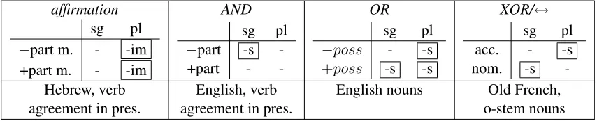
affirmation AND OR XOR/↔

sg pl

−part m. - -im +part m. - -im

sg pl −part -s

-+part -

-sg pl −poss - -s +poss -s -s

sg pl

acc. - -s

nom. -s

-Hebrew, verb English, verb English nouns Old French,

agreement in pres. agreement in pres. o-stem nouns

Figure 2: Patterns of syncretism isomorphic to the structure of Boolean connectives

Bower, 1988) also do not predict the order AND>

OR fore similar reasons. Feldman (2000) speculates that this order is due to a general advantage of the UP-versions of a category over the DOWN-versions (for a category that divides the set of instances into two uneven sets, the UP-version is the version in which the smaller subset is positively labeled, and the DOWN-version is the version in which the larger subset is positively labeled). However, he offers no explanation for this observation. On the other hand, it is known that the choice of representations can af-fect learnability. For instance, k-DNF formulas are not PAC-learnable while k-CNF formulas describing the same class of patterns are PAC-learnable (Kearns and Vazirani, 1994). Interestingly, this result also shows that conjunctive representations have an ad-vantage over the disjunctive ones because a very simple strategy for learning conjunctions (Valiant, 1984) can be extended to the problem of learning k-CNFs. The learner proposed here includes in its core a similar intersective strategy which is respon-sible for deriving the order AND>OR.

The second goal of the paper is to provide a uni-fied account of learning one vs. several categories that partition the feature space (the second problem is the problem of learning paradigms). The most straight-forward way of doing this – treating cate-gory labels as another feature with n values forn

labels – is not satisfactory for several reasons

dis-cussed in section 2. In fact, there is empirical ev-idence that the same pattern is learned differently depending on whether it is presented as learning a distinction between positive and negative instances of a category or whether it is presented as learning two different (non-overlapping) categories. This ev-idence will be discussed in section 3.

I should stress that the learner proposed here is not designed to be a model of “performance.” It makes a number of simplifying assumptions and does not include parameters that are fitted to match the be-havioral data. The main goal of the model is to pre-dict the differences in subjective complexity of cate-gories as a function of their logical structure and the presence/absence of negative examples.

2 Learning one versus many categories

Neutral (AND/ORn) f1 f1

f2 A B

f2 B B

Biased

ANDb ORb

f1 f1

f2 A ¬A

f2 ¬A ¬A

f1 f1

f2 ¬A A

f2 A A

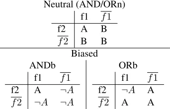
Table 1: Three AND/OR conditions in Gottwald’s study

different morphs are used with exactly the same set of features as well as paradigms with “acciden-tal gaps,” combinations of morpho-syntactic feature values that are impossible in a language. In fact, however, morphs tend to partition the space of pos-sible instances so that no instance is associated with more than one morph. That is, true free variation is really rare (Kroch, 1994). Secondly, system-wide rather than lexical “accidental gaps” are also rare in morphology (Sims, 1996). Therefore, I construe the classification problem in both cases as learning a set of non-overlapping Boolean formulas correspond-ing to categories. This set can consist of just one formula, corresponding to learning a single category boundary, or it can consist of multiple formulas that partition the feature space, corresponding to learn-ing non-overlapplearn-ing categories each associated with a different label.

3 Effects of labeling on category complexity

A study by Gottwald (1971) found interesting dif-ferences in the subjective complexity of learning patterns in figure 1 depending on whether the data was presented to subjects as learning a single cat-egory (stimuli were labeled A vs. ¬A) or whether it was presented as learning two distinct categories (the same stimuli were labeledA vs. B). Follow-ing this study, I refer to learnFollow-ing a sFollow-ingle category as “biased labeling” (abbreviatedb) and learning sev-eral categories as “neutral labeling” (abbreviatedn). Observe that since the AND/OR category divides the stimuli into unequal sets, it has two different biased versions: one biased towards AND and one biased towards OR (as demonstrated in table 1). The order of category complexity found by Gottwald was

AFFn, AFFb>ANDb>AND/ORn>ORb, XORb

>XORn

These results show that for the XOR category the neutral labeling was harder than biased labeling. On the other hand, for the AND/OR category the neutral labeling was of intermediate difficulty, and, interest-ingly, easier than ORb. This is interesting because it goes against an expectation that learning two cat-egories should be harder than learning one category. Pertsova (2012) partially replicated the above find-ing with morphological stimuli (where null vs. overt marking was the analog of biased vs. neutral label-ing). Certain results from this study will be high-lighted later.

4 The learning algorithm

This proposal is intended to explain the complex-ity differences found in learning categories in the lab and in the real world (as evinced by typologi-cal facts). I focus on two factors that affect category complexity, the logical structure of a category and the learning mode. The learning mode refers to bi-ased vs. neutral labeling, or, to put it differently, to the difference between learning a single category and learning a partition of a feature space into sev-eral categories. The effect of the learning mode on category complexity is derived from the following two assumptions: (i) the algorithm only responds to negative instances when they contradict the current grammar, and (ii) a collection of instances can only be referred to if it is associated with a positive label. The first assumption is motivated by observations of Bruner et. al (1956) that subjects seemed to rely less on negative evidence than on positive evidence even in cases when such evidence was very informative. The second assumption corresponds to a common sentiment that having a linguistic label for a cate-gory aids in learning (Xu, 2002).

4.1 Some definitions

non-contradictory Boolean formulaφ.1 Namely,φ

describes a set of instancesXif and only if it is log-ically equivalent to the disjunction of all instances inX. For instance, in the world with three binary featuresp, q, w, the formulap∧q describes the set of instances{{pqw},{pqw¯}}(where each instance is represented as a set). We will say that a formula

ψsubsumesa formulaφif and only if the set of in-stances that ψ describes is a superset of the set of instances thatφdescribes. An empty conjunction∅ describes the set of all instances.

The goal of the learner is to learn a set of Boolean formulas describing the distribution of positive la-bels (in the neutral mode all lala-bels are positive, in the biased mode there is one positive label and one negative label). A formula describing the distribu-tion of a labellis encoded as a set of entries of the formeli (an i-th entry for labell). The distribution

oflis given byel1 ∨. . .∨eln, the disjunction ofn

formulas corresponding to entries forl. Each entry

eli consists of two components: a maximal

conjunc-tion φmax and an (optional) list of other formulas

EX (for exceptions). A particular entryewith two components,e[φmax]ande[EX] ={φ1. . . φn}, de-fines the formulae[φmax]∧ ¬(φ1∨φ2∨. . .∨φn).

e[φmax] can intuitively be thought of as a rule of thumb for a particular label andEX as a list of ex-ceptions to that rule. In the neutral mode exex-ceptions are pointers to other entries or, more precisely, for-mulas encoded by those entries. In the biased mode they are formulas corresponding to instances (i.e., conjunctions of feature values for all features). The algorithm knows which mode it is in because the bi-ased mode contains negative labels while the neutral mode does not. Finally, an instanceiis consistent with an entry e if and only if the conjunction en-coded byilogically implies the formula encoded by

e. For example, an instance{pqw}is consistent with an entry encoding the formula{p}.

Note that while this grammar can describe arbi-trarily complex patterns/partitions, each entry in the neutral learning mode can only describe what lin-guistics often refer to as “elsewhere” patterns (more precisely Type II patterns in the sense of Pertsova (2011)). And thee[φmax]component of each entry

1_{The set of Boolean formulas is obtained by closing the set}

of feature values under the operations of conjunction, negation, and disjunction.

by definition can only describe conjunctions. There are additional restrictions on the above grammar: (i) the exceptions cannot have a wider distribution than “the rule of thumb” (i.e., an entry el cannot corre-spond to a formula that does not pick out any in-stances), (ii) no loops in the statement of exceptions is possible: that is, if an entry A is listed as an ception to the entry B, then B cannot also be an ex-ception for A (a more complicated example of a loop involves a longer chain of entries).

When learning a single category, there is only one entry in the grammar. In this case arbitrarily complex categories are encoded as a complement of some conjunction with respect to a number of other conjunctions (corresponding to instances).

4.2 General description

The general organization of the algorithm is as fol-lows. Initially, each positive label is assumed to cor-respond to a single grammatical entry, and theφmax component of this entry is computed incrementally through an intersective generalization strategy that extracts features invariant across all instances used with the same label. When the grammar overgener-alizes by predicting two different labels for at least one instance, exceptions are introduced. The pro-cess of exception listing can also lead to overgener-alizations if exceptions are pointers to other entries in the grammar. When these overgeneralizations are detected the algorithm creates another entry for the same label. This latter process can be viewed as positing homophonous entries when learning form-meaning mappings, or as creating multiple “clus-ters” for a single category as in the prototype model SUSTAIN (Love et al., 2004), and it corresponds to explicitly positing a disjunctive rule. Note that if exceptions are not formulas for other labels, but in-dividual instances, then exception listing does not lead to overgeneralization and no sub-entries are in-troduced. Thus, when learning a single category the learner generalizes by using an intersective strategy, and then lists exceptions one-by-one as they are dis-covered in form of negative evidence.

simple distributions of data. (Subclasses of Boolean formulas are efficiently learnable in various learning frameworks (Kearns et al., 1994).) If the learning al-gorithm can easily learn certain patterns (providing an explanation for what patterns and distributions count as simple), we do not need to require that it be in general efficient.

4.3 Detailed description

First I describe how the grammar is updated in re-sponse to the data. The update routine uses a strat-egy that in word-learning literature is called cross-situational inference. This strategy incrementally fil-ters out features that change from one instance to the next and keeps only those features that remain invariant across the instances that have the same la-bel. Obviously, this strategy leads to overgeneral-izations, but not if the category being learned is an affirmation or conjunction. This is because affirma-tions and conjuncaffirma-tions are defined by a single set of feature values which are shared by all instances of a category (for proof see Pertsova (2007) p. 122). Af-ter the entry for a given label has been updated, the algorithm checks whether this entry subsumes or is subsumed by any other entry. If so, this means that there is at least one instance for which several labels are predicted to occur (there is competition among the entries). The algorithm tries to resolve competi-tion by listing more specific entries as excepcompeti-tions to the more general ones.2 However there are cases in which this strategy will either not resolve the com-petition, or not resolve it correctly. In particular, the intermediate entries that are in competition may be such that neither subsumes the other. Or after updating the entries using the intersective strategy one entry may be subsumed by another based on the instances that have been seen so far, but not if we take the whole set of instances into account. These cases are detected when the predictions of the cur-rent grammar go against an observed stimulus (step 11 in the function “Update” below). Finally, excep-tion listing fails if it would lead to a “loop” (see

sec-2_{This idea is familiar in linguistics from at least the times of}

P¯anini. In Distributed Morphology, it is referred to as the Subset Principle for vocabulary insertion (Halle and Marantz, 1993). Similar principles are assumed in rule-ordering systems and in OT (i.e., more specific rules/constraints are typically ordered before the more general ones).

tion 4.1). The XOR pattern is an example of a simple pattern that will lead to a loop at some point during learning. In general this happens whenever the dis-tribution of the two labels are intertwined in such a way that neither can be stated as a complement of the invariant features of the other.

The following function is used to add an excep-tion:

AddException(expEntry, ruleEntry):

1. ifaddingexpEntrytoruleEntry[EX]leads to a loopthenFAIL

2. elseaddexpEntrytoruleEntry[EX]

The routine below is called within the main func-tion (presented later); it is used to update the gram-mar in response to an observed instancex with the labelli(the index of the label is decided in the main function).

Update

Input: G (current grammar); x (an observed in-stance),li(a label for this instance)

Output: newG 1: newG←G

2: if∃eli ∈newGthen

3: eli[φmax]←eli[φmax]∩x

4: else

5: add the entry eli to newG with values eli[φmax] =x;eli[EX] ={}.

6: for alle_l0

j ∈newG(el 0

j 6=eli)do

7: ife_l0

j subsumeseli then

8: AddException(eli, el0_j)

9: else ifeli subsumesel0jthen

10: AddException(el0 j, eli)

11: if∃e_l0

j ∈newG(l

0 _{6=l) such thatxis consistent}

withel0 j then

12: AddException(eli, el0_j)

Before turning to the main function of the algo-rithm, it is important to note that because a grammar may contain several different entries for a single la-bel, this creates ambiguity for the learner. Namely, in case a grammar contains more than one entry for some label, say twoAlabels, the learner has to de-cide after observing a datum(x, A), which entry to update,eA1 oreA2. I assume that in such cases the

current instance, where similarity is calculated as the number of features shared betweenxandeAi[φmax]

(although other metrics of similarity could be ex-plored).

Finally, I would like to note that the value of an entryel(x)can change even if the algorithm has not updated this entry. This is because the value of some other entry that is listed as an exception in el(x) may change. This is one of the factors contributing to the difference between the neutral and the biased learning modes: if exceptions themselves are entries for other labels, the process of exception listing be-comes generalizing.

Main

Input: an instance-label pair (x, l), previous hy-pothesisG(initially set to an empty set) Output: newG (new hypothesis)

1: setEto the list of existing entries for the labell

inG

2: k← |E| 3: ifE6={}then

4: setelcurr toeli ∈Ethat is most similar tox

5: E ←E−elcurr

6: else

7: curr←k+ 1

8: if l is positiveand (¬∃elcurr ∈ Gor x is not

consistent withelcurr)then

9: ifupdate(G, x, lcurr)failsthen 10: goto step 3

11: else

12: newG←update(G, x, lcurr)

13: else iflis negative and there is an entryein G consistent withx(positive label was expected) then

14: addx toe[EX]and minimizee[EX]to get

newG

Notice that the loop triggered when updatefails is guaranteed to terminate because when the list of all entries for a labell is exhausted, a new entry is introduced and this entry is guaranteed not to cause

updateto fail.

This learner will succeed (in the limit) on most presentations of the data, but it may fail to converge on certain patterns if the crucial piece of evidence needed to resolve competition is seen very early on and then never again (it is likely that a human learner would also not converge in such a case).

This algorithm can be additionally augmented by a procedure similar to the selective attention mech-anism incorporated into several psychological mod-els of categorization to capture the fact that certain hard problems become easy if a subject can ignore irrelevant features from the outset (Nosofsky et al., 1994a). One (not very efficient, but easy) way to incorporate selective attention into the above algo-rithm is as follows. Initially set the number of rel-evant featureskto 1. Generate all subsets ofF of length k, select one such subset Fk and apply the above learning algorithm assuming that the feature space isFk. When processing a particular instance, ignore all of its features except those that are inFk. If we discover two instances that have the same as-signment of features inFkbut that appear with two different labels, this means that the selected set of features is not sufficient (recall that free variation is ruled out). Therefore, when this happens we can start over with a new Fk. If all sets of length k have been exhausted, increase k to k+ 1 and re-peat. As a result of this change, patterns definable by smaller number of features would generally be easier to learn than those definable by larger number of features.

5 Predictions of the model for learning Boolean connectives

We can evaluate predictions of this algorithm with respect to category complexity in terms of the pro-portion of errors it predicts during learning, and in terms of the computational load, roughly measured as the number of required runs through the main loop of the algorithm. Recall that a single data-point may require several such runs if the update routine fails and a new sub-category has to be created.

Below, I discuss how the predictions of this al-gorithm compare to the subjective complexity rank-ing found in Gottwald’s experiment. First, consider the relative complexity order in the neutral learning mode: AFF>AND/OR>XOR.

overgener-alization of the label associated with the disjunctive category to the rest of the instances. This will hap-pen if the OR part of the pattern is processed before the AND part. When learning an XOR pattern, the learner is guaranteed to overgeneralize one of the labels on any presentation of the data. Let’s walk through the learning of the XOR pattern, repeated below for convenience.

f1 f1

f2 A B

f2 B A

Suppose for simplicity that the space of features includes only f1 and f2, and that the first two ex-amples that the learner observes are(A,{f1, f2}) and (A,{f1, f2}). After intersecting {f1, f2} and {f1, f2} the learner will overgeneralize A

to the whole paradigm. If the next example is (B,{f1, f2}), the learner will partially correct this overgeneralization by assuming thatAoccurs every-where except every-whereB does (i.e., except{f1, f2}). But it will continue to incorrectly predict A in the remaining fourth cell that has not been seen yet. WhenBis observed in that cell, the learner will at-tempt to update the entry for B through the inter-section but this attempt will fail (because the en-try for B will subsume the enen-try for A, but we can’t list A as an exception for B since B is al-ready listed as an exception for A). Therefore, a new sub-entry for B, {f1, f2}, will be introduced and listed as another exception forA. Thus, the fi-nal grammar will contain entries corresponding to these formulas: B : (f1 ∧f2)∨(f1 ∧f2) and

A:¬((f1∧f2)∨(f1∧f2)).

Overall the error pattern predicted by the learner is consistent with the order AFF > AND/OR >

XOR.

I now turn to a different measure of complexity based on the number of computational steps needed to learn a pattern (where a single step is equated to a single run of the main function). Note that the speed of learning a particular pattern depends not only on the learning algorithm but also on the distribution of the data. Here I will consider two possible proba-bility distributions which are often used in catego-rization experiments. In both distributions the stim-uli is organized in blocks. In the first one (which I call “instance balanced”) each block contains all possible instances repeated once; in the second

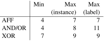
dis-tribution (“label balanced”) each block contains all possible instances with the minimum number of rep-etitions to insure equal numbers of each label. The distributions differ only for those patterns that have an unequal number of positive/negative labels (e.g., AND/OR). Let us now look at the minimum and maximum number of runs through the main loop of the algorithm required for convergence for each type of pattern. The minimum is computed by finding the shortest sequence of data that leads to convergence and counting the number of runs on this data. The maximum is computed analogously by finding the longest sequence of data. The table below summa-rizes min. and max. number of runs for the feature space with 3 binary features (8 possible instances) and for two distributions.

Min Max Max

(instance) (label)

AFF 4 7 7

AND/OR 4 8 11

XOR 7 9 9

Table 2: Complexity in the neutral mode

The difference between AFF and AND/OR in the number of runs to convergence is more obvi-ous for the label balanced distribution. On the other hand, the difference between AND/OR and XOR is clearer for the instance balanced distribution. This difference is not expected to be large for the label balanced distribution, which is not consistent with Gottwald’s experiment in which the stimuli were label balanced, and neutral XOR was significantly more difficult to learn than any other condition.

We now turn to the biased learning mode. Here, the observed order of difficulty was: AFFb>ANDb

>ORb, XORb. In terms of errors, both AFFb and ANDb are predicted to be learned with no errors since both are conjunctive categories. ORb is pre-dicted to involve a temporary overgeneralization of the positive label to the negative contexts. The same is true for XORb except that the proportion of errors will be higher than for ORb (since the latter category has fewer negative instances).

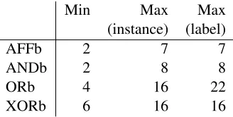
balanced) is given below. Notice that the minimum numbers are lower than in the previous table because in the biased mode some categories can be learned from positive examples alone.

Min Max Max

(instance) (label)

AFFb 2 7 7

ANDb 2 8 8

ORb 4 16 22

XORb 6 16 16

Table 3: Complexity in the biased mode

The difference between affirmation and conjunc-tion is not very large which is not surprising (both are conjunctive categories). Again we see that the two types of distributions give us slightly different predictions. While ANDb seems to be learned faster than ORb in both distributions, it is not clear whether and to what extent ORb and XORb are on average different from each other in the label balanced dis-tribution. Recall that Gottwald found no significant difference between ORb and XORb (in fact numer-ically ORb was harder than XORb). Interestingly, in a morphological analogue of Gottwald’s study in which the number of instances rather than labels was balanced, I found the opposite difference: ORb was easier to learn than XORb (the number of people to reach learning criterion was 8 vs. 4 correspondingly) although the difference in error rates on the testing trials was not significant (Pertsova, 2012). More testing is needed to confirm whether the relative dif-ficulty of these two categories is reliably affected by the type of distribution as predicted by the learner.3

Finally, we look at the effect of labeling within each condition. In the AFF condition, Gottwald found no significant difference between neutral la-beling and biased lala-beling. This could be due to the fact that subjects were already almost at ceiling

3

Another possible reason for the fact that Gottwald did not find a difference between ORb and XORb is this: if selective at-tention is used during learning, it will take longer for the learner to realize that ORb requires the use of two features compared to XORb especially when the number of positive and negative ex-amples are balanced. In particular, a one feature analysis of ORb can explain 5/6 of the data with label balanced stimuli, while a one feature analysis of XORb can only explain 1/2 of the data, so it will be quickly abandoned.

in learning this pattern (median number of trials to convergence for both conditions was ≤ 5). In the AND/OR condition, Gottwald observed the interest-ing order ANDb >AND/OR > ORb. This order is also predicted by the current algorithm. Namely, the neutral category AND/OR is predicted to be harder than ANDb because (1) ANDb requires less computational resources (2) on some distributions of data overgeneralization will occur when learn-ing an AND/OR pattern but not an ANDb category. The AND/OR>ORb order is also predicted and is particularly pronounced for label balanced distribu-tion. Since two labels are available when learning the AND/OR pattern, the AND portion of the pat-tern can be learned quickly and subsequently listed as an exception for the OR portion (which becomes the“elsewhere” case). On the other hand, when learning the ORb category, the conjunctive part of the pattern is initially ignored because it is not as-sociated with a label. The learner only starts paying attention to negative instances when it overgeneral-izes. For a similar reason, the biased XOR category is predicted to be harder to learn than the neutral XOR category. This latter prediction is not consis-tent with Gottwald’s finding, who found XORn not just harder than other categories but virtually impos-sible to learn: 6 out of 8 subjects in this condition failed to learn it after more than 256 trials. In con-trast to this result (and in line with the predictions of the present learner), Pertsova (2012) found that the neutral XOR condition was learned by 8 out of 12 subjects on less than 64 trials compared to only 4 out of 12 subjects in the biased XOR condition.

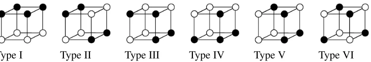
Type I Type II Type III Type IV Type V Type VI

Figure 3: Shepard et. al. hierarchy

6 Other predictions

Another well-studied hierarchy of category com-plexity is the hierarchy of symmetric patterns (4 pos-itive and 4 negative instances) in the space of three binary features originally established by Shepard et. al (1961). These patterns are shown in figure 3 us-ing cubes to represent the three dimensional feature space.

Most studies find the following order of complex-ity for the Shepad patterns: I>II>III, IV, V>VI (Shepard et al., 1961; Nosofsky et al., 1994a; Love, 2002; Smith et al., 2004). However, a few studies find different rankings for some of these patterns. In particular, Love (2002) finds IV>II with a switch to unsupervised training procedure. Nosofsky and Palmeri (1996) find the numerical order I>IV>III

>V>II>VI with intergral stimulus dimensions (feature values that are difficult to pay selective at-tention to independent of other features, e.g., hue, brightness, saturation). More recently Moreton and Persova (2012) also found the order IV >III>V, VI (as well as I>II, III,>VI) in an unsupervised phonotactics learning experiment.

So, one might wonder what predictions does the present learner make with respect to these patterns. We already know that it predicts Type I (affirmation) to be easier than all other types. For the rest of the patterns the predictions in terms of speed of acquisi-tion are II>III>IV, V>VI in the neutral learning mode (similar to the typical findings). In the biased learning mode, patterns II through VI are predicted to be learned roughly at the same speed (since all re-quire listing four exceptions). If selective attention is used, Type II will be the second easiest to learn after Type I because it can be stated using only two features. However, based on the error rates, the order of difficulty is predicted to be I>IV>III>V>

II>VI (similar to the order found by Nosofsky and Palmeri (1996)). No errors are ever made with Type

I. The proportion of errors in other patterns depends on how closely the positive examples cluster to each other. For instance, when learning a Type VI pattern (in the biased mode) the learner’s grammar will be correct on 6 out of 8 instances after seeing any two positive examples (the same is not true for any other pattern, although it is almost true for III). After see-ing the next instance (dependsee-ing on what it is and on the previous input) the accuracy of the grammar will either stay the same, go up to 7/8, or go down to 1/2. But the latter event has the lowest probability. Note that this learner predicts non-monotonic behav-ior: it is possible that a later grammar is less accurate than the previous grammar. So, for a non-monotonic learner the predictions based on the speed of acqui-sition and accuracy do not necessarily coincide.

There are many differences across the categoriza-tion experiments that may be responsible for the dif-ferent rankings. More work is needed to control for such differences and to pin down the sources for dif-ferent complexity results found with the patterns in figure 3.

7 Summary

The current proposal presents a unified account for learning a single category and a set of categories par-titioning the stimuli space. It is consistent with many predictions about subjective complexity rankings of simple categories, including the ranking AND >

OR, not predicted by most categorization models, and the difference between the biased and the neu-tral learning modes not previously modeled to my knowledge.

References

George N. Clements. 2003. Feature economy in sound systems. Phonology, 20(3):287–333.

Michael Cysouw. 2003. The paradigmatic structure of person marking. Oxford studies in typology and lin-guistic theory. Oxford University Press, Oxford. V´ıctor Dalmau. 1999. Boolean formulas are hard to

learn for most gate bases. In Osamu Watanabe and Takashi Yokomori, editors,Algorithmic Learning The-ory, volume 1720 ofLecture Notes in Computer Sci-ence, pages 301–312. Springer Berlin / Heidelberg. Jacob Feldman. 2000. Minimization of Boolean

com-plexity in human concept learning. Nature, 407:630– 633.

Mark A. Gluck and Gordon H. Bower. 1988. evaluating an adaptive network model of human learning. Jour-nal of memory and language, 27:166–195.

Richard L. Gottwald. 1971. Effects of response labels in concept attainment. Journal of Experimental Psychol-ogy, 91(1):30–33.

Morris Halle and Alec Marantz. 1993. Distributed mor-phology and the pieces of inflection. In K. Hale and S. J. Keyser, editors,The View from Building 20, pages 111–176. MIT Press, Cambridge, Mass.

Michael Kearns and Umesh Vazirani. 1994. An intro-duction to computational learning theory. MIT Press, Cambridge, MA.

Michael Kearns, Ming Li, and Leslie Valiant. 1994. Learning boolean formulas. J. ACM, 41(6):1298– 1328, November.

Anthony Kroch. 1994. Morphosyntactic variation. In Katharine Beals et al., editor, Papers from the 30th regional meeting of the Chicago Linguistics Soci-ety: Parasession on variation and linguistic theory. Chicago Linguistics Society, Chicago.

Bradley C. Love, Douglas L. Medin, and Todd M. Gureckis. 2004. SUSTAIN: a network model of cat-egory learning. Psychological Review, 111(2):309– 332.

Bradley C. Love. 2002. Comparing supervised and unsu-pervised category learning. Psychonomic Bulletin and Review, 9(4):829–835.

Jeff Mielke. 2004. The emergence of distinctive features. Ph.D. thesis, Ohio State University.

Elliott Moreton and Katya Pertsova. 2012. Is phonolog-ical learning special? Handout from a talk at the 48th Meeting of the Chicago Society of Linguistics, April. Ulrich Neisser and Paul Weene. 1962. Hierarchies in

concept attainment. Journal of Experimental Psychol-ogy, 64(6):640–645.

Robert M. Nosofsky and Thomas J. Palmeri. 1996. Learning to classify integral-dimension stimuli. Psy-chonomic Bulletin and Review, 3(2):222–226.

Robert M. Nosofsky, Mark A. Gluck, Thomas J. Palmeri, Stephen C. McKinley, and Paul Gauthier. 1994a. Comparing models of rule-based classification learn-ing: a replication and extension of Shepard, Hov-land, and Jenkins (1961). Memory and Cognition, 22(3):352–369.

Robert M. Nosofsky, Thomas J. Palmeri, and Stephen C. McKinley. 1994b. Rule-plus-exception model of clas-sification learning. Psychological Review, 101(1):53– 79.

Katya Pertsova. 2007. Learning Form-Meaning Map-pings in the Presence of Homonymy. Ph.D. thesis, UCLA.

Katya Pertsova. 2011. Grounding systematic syncretism in learning. Linguistic Inquiry, 42(2):225–266. Katya Pertsova. 2012. Logical complexity in

morpho-logical learning. In Proceedings of the 38th Annual Meeting of the Berkeley Linguistics Society.

Roger N. Shepard, C. L. Hovland, and H. M. Jenkins. 1961. Learning and memorization of classifications.

Psychological Monographs, 75(13, Whole No. 517). Andrea Sims. 1996. Minding the Gaps: inflectional

defectiveness in a paradigmatic theory. Ph.D. thesis, The Ohio State University.

J. David Smith, John Paul Minda, and David A. Wash-burn. 2004. Category learning in rhesus monkeys: a study of the Shepard, Hovland, and Jenkins (1961) tasks. Journal of Experimental Psychology: General, 133(3):398–404.

Leslie G. Valiant. 1984. A theory of the learnable. In

Proceedings of the sixteenth annual ACM symposium on Theory of computing, STOC ’84, pages 436–445, New York, NY, USA. ACM.