Dynamic Memory Efficient Frequent Pattern Growth for Data Excavation

32

Dynamic Memory Efficient Frequent Pattern Growth for

Data Excavation

G. Gunasekaran

Assistant Professor of Computer Science

Nehru Memorial College

Puthnampatti, Trichy

S. Murugan,

PhD

Associate Professor of Computer Science

Nehru Memorial College

Puthnampatti, Trichy

ABSTRACT

Advancements in information technology increase the data volume of many domains into manyfold. Dynamic Memory Efficient Frequent Pattern (DMEFP) technique introduces new methods to represent data and redundant frequent patterns. Introduction of Repeat Pattern Table (RPT) and new node type ‘Tree Pattern Node’ (TPN) in frequent pattern tree softens the data mining process to be performed in a modern way. DMEFP technique comprises new rules to aggregate pattern nodes and RPT. Computational resources are used sagely in DMEFP technique for data mining. Reduced resource consumption helps to parse large amount of data in short time durations without much complexity.

Keywords

Information Technology, Data Mining, FP-Growth, Frequent Pattern Tree, Memory efficient data mining

1. INTRODUCTION

Finding correlations between associated data create a valuable cognition. Modern databases are huge in volume and require complex procedures for parsing. Data mining techniques are designed to perform deviation detection, dependency modelling (association rule learning), clustering, classifying, regression and summarization. Association rules are used to relate data items in a procedural way. Deviation detection otherwise called as Anomaly detection is a process of identifying unusual records in a dataset. An anonymous record requires special investigation to find whether the transaction is occurred by mistake or a special rule has to be introduced to validate the record. Dependency modelling is used to define the relationships between the variables in the transaction records. Clustering is used to find and organize same or similar group of records under a common label. Classification procedure is used to identify a new record based on the existing known structures created by clustering. Regression is used to introduce a common function to correlate the data of same group with no or least errors. This is used to estimate the relationships within records or datasets. Summarization is used to enable data structure visualizations and to produce reports based on different requirements.

2. EXISTING SYSTEMS

2.1 Apriori

Apriori[1] is a standard well known procedure for extracting association rules from binary transaction databases. Apriori starts with a frequent individual item in a dataset and broadens it to the frequent item sets in a dataset. In Apriori algorithm, the frequency of the item sets are handled using a threshold value of C. Apriori uses ‘Candidate Generation’ a bottom-up approach to extend a single frequent item into frequent item

sets. This process continues until there are no successful

Candidate Generations. Candidate Item sets’ count is

calculated using Hash-Tree structure and breath-first-search by Apriori. It can generate candidate item set with length of k

from item set length k-1. Then the frequent item sets are determined from the candidates.

If T is a transaction database with support threshold ∈ then the pseudo code for Apriori will be

Apriori(𝑇, 𝜖)

L1 = { Large 1 – itemsets } K= 2

while 𝐿𝑘−1≠ ∅

𝐶𝑘 = 𝑎𝑈 𝑏 𝑎𝜖 𝐿𝑘−1∧ 𝑏 ∉ 𝑎} − {𝑐| 𝑠 𝑠 ⊆ 𝑐 ∧

s = 𝑘 − 1} ⊈ 𝐿𝑘−1}

for transactions 𝑡 ∈ 𝑇

𝐶𝑡 = { 𝑐 | 𝑐 ∈ 𝐶𝑘 ∧ 𝑐 ⊆ 𝑡 }

for candidates 𝑐 ∈ 𝐶𝑡

count[c] = count[c] + 1

𝐿𝑘 = {c|c ∈ 𝐶𝑘∧ 𝑐𝑜𝑢𝑛𝑡 𝑐 ≥ ∈ }

k = k + 1

return ⋃

𝑘𝐿𝑘

where 𝐶𝑘 is the candidate set for level 𝑘.

In Apriori algorithm, Candidate Generation is a resource consuming process that involves large number of subsets scans. Bottom-up approach in breadth-first traversal can find maximum subset count only after finding all 2 𝑠 _{− 1 proper}

subsets. This disadvantage makes it difficult to use Apriori algorithm with larger database. To overcome this issue some other procedures are introduced.

2.2 FP-Growth

33 no items in common between transactions, then the size of the

FP-Tree will be as large as the actual data. FP-Tree Structure:

1. Root Node (Null Node) which holds item-prefix sub-trees is used to initializes tree structure

2. Each item prefix sub-tree node consists three fields {Item Name, Count, Next Node Link}

3. Frequent-Item-header table consists of two fields {Item Name, Link to first node}

4. Frequent –Item-header table has optional support count for an item

FP-Tree Construction Pseudo code:

FPTree ConstructFPTree(Transaction Database DB)

1. Perform DB scan, Accumulate F (set of frequent items) and the support of each frequent item. Sort F in support-descending order in the list of frequent items named FList

2. Initialize Tree with Root Node T (null Node)

3. For each transaction Trans in DB do the following:

i. Assort frequent items from transactions and sort them based on the order of FList.

ii. Represent sorted frequent-item list as [p | P], where p is the first element and P is the remaining list

iii. If T has a child N then item-name = p

N = N+1

Else Create new node N with count 1 iv. Repeat step iii recursively for full database

The size of the FP-Tree depends on the order of the items. Therefore the memory consumption of FP-Growth is very high in general when large databases are involved.

2.3. ECLAT

Eclat[5] is recursively defined procedure to perform item set mining that is used to frequent pattern identification. These frequent patterns are also called as association rules. Eclat uses Tidset[6] intersections to compute candidate item set support count and avoids generation of candidate subsets those are not present in prefix tree.

The initial Eclat call uses all the single item sets with their transaction IDs (tids). Then the recursive calls are initialized to verify all itemset-tidset pair 𝑋, 𝑡 𝑋 with other pairs 𝑌, 𝑡 𝑌 to generate new candidates 𝑁𝑋𝑌. Whenever the new

candidates is found to be frequent, then it is added with set 𝑃𝑋.

Pseudo code: 1. Let S be an Item set

2. T is the transaction tag

3. Multiset transaction U = 𝑋 ∈ 𝑇 𝑆 ⊆ 𝑡

4. Absolute Support of S = 𝑈 = | 𝑋 ∈ 𝑇 𝑆 ⊆ 𝑡 |

5. Relative support of S = 𝑈 ∕ 𝑇 ∗ 100%; where 𝑈 and 𝑇 are the number of elements in U and T respectively

6. The anti-monotone support is ∀ 𝐼, 𝐽: 𝐽 ⊆ 𝐼 = (supp 𝐽 ≥ supp 𝐼 )

Eclat’s Depth-First-Search procedure and its vertical database layout causes more time for intersection of Tidlists. When the database is considerably large, the memory consumption of Eclat’s is large and occupying other computational resources makes it less manageab

le.

2.4 DFEM

DFEM[7] refers Dynamic FP-Tree and Eclat Method. It uses both FP-Growth and Eclat algorithms for mining. A threshold value is used to determine the switching process between FP-Growth and Eclat algorithm. DFEM has four major modules, they are Construction of FP-Tree, Mining FP-Tree, Mining Bit Vector and updating the threshold.

FP-Tree Construction Procedure:

1. Find frequent items by scanning the database 2. Construct FP-Tree based on the scan results

3. Call FP-Tree Mining

FP-Tree Mining Procedure:

1. If FP-Tree has a single path, then all combinations of X nodes P = X ∪ suffix

2. For all Items of Y in the header table P = Y ∪ suffix

3. Construct Conditional pattern of Y based on C

4. If number of nodes in Y > K, then construct Y’s conditional FP-Tree and call FP-Mining Procedure recursively

5. Else transform C into Bit Vector V, Weight Vector W and call Bit Vector Mining

Bit Vector Mining Procedure:

1. Arrange V based on its item support in descending order

2. For each vector 𝑣𝑖 in V

Output = 𝑣𝑖 ∪ suffix

3. For each vector 𝑣𝑘 in V, where k<i

𝑢𝑘= 𝑣𝑖 AND 𝑣𝑘

4. 𝑠𝑢𝑝𝑘 = support of 𝑢𝑘 based on weight 𝑤

5. If all 𝑢𝑘 in U are identical to 𝑣𝑖, then for each combination

of X in U output = X ∪ output

else if U is empty, then call Bit Vector Mining again

Threshold updating procedure:

In DFEM, FP-Tree mining[8] has a set of values of threshold K as K= 𝑘₀, 𝑘1…𝑘𝑛 . The difference between previous pattern

𝑃𝑖−1 and current pattern 𝑃𝑖 is represented as 𝑅𝑖. 𝑅𝑖 is

calculated as

𝑅𝑖=

𝑃𝑖−1

𝑃𝑖, 𝑖 = 1 𝑡𝑜 𝑁

34 Threshold updating pseudo code:

1. If Update K called for the first time

Then Create an array P with N elements. 2. Initialize the array with zero

3. For i=0 to N-1

If size > I * size then 𝑃𝑖 = 𝑃𝑖 + New

Pattern

Else exit loop

4. Initalize K as Zero (K=0) 5. For i=N-1 to 1

If 𝑅𝑖≥ 2 then K=(i+1) * step

6. exit loop

DFEM is quicker and more accurate than the previous methods. But the memory consumption is comparatively high when dealing with a larger size database.

2.5 MEFP

Memory Efficient Frequent Pattern mining[9][10] uses transposition of database. The space complexity of MEFP is 𝑂 𝑛 and the longest common sequence space complexity is 𝑂 𝑛2 _{. The time consumption of MEFP is 𝑂 𝑚𝑛 . It uses X}

data or Y data based on the quantity of support counts. The space is either 𝑂 𝑚 or 𝑂 𝑛 whichever is smaller.

MEFP Procedure:

1. Convert Database DB into Transpose Form DT

2. Compute F1 for all frequent Items

3. C1 = DT [Frequent Item Row with Transaction ID String]

4. Assign K=2

5. While Lk-1 ≠ {𝐾} do

Compute 𝐶𝑘 for all candidates k-1 item sets

Compute Lk = APS(𝐶𝑘)

Increment the value of K by 1

In MEFP, there is a need to shift rows and columns and X-Y variable values interchanging[11][12] takes more time. Even though MEFP consumes lesser memory, the time for formatting frequent patterns and generating corresponding association rules takes more time for larger databases.

3. PROPOSED METHOD

Dynamic Memory Efficient Frequent Pattern (DME-FP) procedure introduces a new node type named Tree Pattern Node (TPN). It also introduces Repeat Pattern Table (RPT) – a table to manage TPN. This procedure is designed with caution to handle computational resources[13][ like memory[14] and time[15] with improved basic metrics of a data mining procedure of accuracy, precision and recall.

Table 1 contains a transaction history with different item sets of items {a, b, c, d, e, j, k, l, m, n}. As given in table, the transactions can be any possible combination of the taken items.

Table 1

TID Items

1 {a,b}

2 {b,c,d}

3 {a,c,d,e}

4 {a,d,e}

5 {a,b,c}

6 {a,b,c,d}

7 {a}

8 {a,b,c}

9 {a,b,d}

10 {b,c,e}

11 {c,j,k}

12 {c,k,l,m}

13 {c,j,l,m,n}

14 {c,j,m,n}

15 {c,j,k,l}

16 {c,j,k,l,m}

17 {c,j}

18 {c,j,k,l}

19 {c,j,k,m}

20 {c,k,l,n}

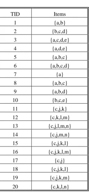
35 Figure 1

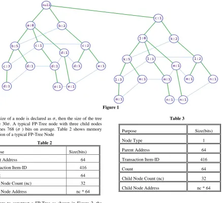
If the size of a node is declared as 𝜎, then the size of the tree will be 30𝜎. A typical FP-Tree node with three child nodes consumes 768 (𝜎 ) bits on average. Table 2 shows memory allocation of a typical FP-Tree Node

Table 2

Purpose Size(bits)

Parent Address 64

Transaction Item-ID 416

Count 64

Child Node Count (nc) 32

Child Node Address nc * 64

Therefore to construct a FP-Tree as shown in Figure 2, the memory consumption will be 23040 Bytes. This implies to handle twenty transactions with ten different items FP-Tree method requires 2880 Bytes of memory. Modern databases contain vast number of items with large number of transactions. To organize a complete database into FP-Tree for analysis will be a memory starving process.

Proposed DME-FP uses a different type of tree nodes. Since DME-FP has an additional node type of TPN, one more field with single bit length is added with the default FP-Tree Node. So the size of a DME-FP node will be 769 bits. DME-FP node architecture is given in Table 3

Table 3

Purpose Size(bits)

Node Type 1

Parent Address 64

Transaction Item-ID 416

Count 64

Child Node Count (nc) 32

Child Node Address nc * 64

The Node Type field will have the value 0 is to represent a regular node and 1 is to represent a Tree Pattern Node. In DME-FP, a RPT consists of four fixed length fields and a variable length field. Pattern ID, Root Node ID, Number of nodes in BFS and Number of Substitute Items Count are fixed with 16 bits, 64 bits, 8 bits and 4 bits respectively. The Number of nodes in BFS filed can hold up to 255 refers a pattern can have

255 nodes maximum including the root node. The fifth variable length field is based on the fourth field Substitute Item Count. If the value of Substitute Item count is 𝜂 then the size of fifth filed will be 𝜂 × 416 bits. Since the size of Substitute Item Count is limited to 4 bits, the value of 𝜂 can go up to 16. This refers the number of substitute items can be 16 at maximum.

For the transaction history as in Table 1, Repeat Pattern Table will be generated as follows

Pattern

ID

Root Node ID

Number of Nodes

on BFS

Substitute Item

Count

36 Figure 2

The size of this RPT is 1664 bits. The DME-FP tree representation for the transaction history is shown in Figure 2.

This DME-FP Tree the size of 15 regular nodes is 11535 bits, the size of 1 tree pattern node is 577 bits and the size of RPT is 1664 bits. In total, the DME-FP tree consumes 13776 bits (12112 bits for tree + 1664 for RPT) whereas regular FP-Tree consumes 23040 bits for the same transaction history. Content of tree pattern node PN1 is given in table 4.

Overall memory preservation of DME-FP over regular FP-Tree is 9264 bits (1158 Bytes). This proves using DME-FP saves greater than 1KB of memory for a 20 item set transaction history.

Table 4

Field Value Size (Bits)

Node Type 1 1

Parent Address Address(null) 64

Transaction

Item ID 11 416

Count 1 64

Child Node

Count 0 32

Child Node

Address 0 0

Total Size 577

4. EXPERIMENTAL SETUP

To evaluate the performance of DME-FP procedure, benchmark datasets Chess, Kosarak, Mushroom, pumbsb_star, Retail and T10I4D100K are used. Accuracy, Precision, Recall, Processing Time and Memory are measured with noted datasets and for a comparative analysis, existing methods Apriori, FP-Growth, Eclat, DFEM and MEFP are taken. The processing time and memory consumption are measured in a computer with Processor 2.4 GHz i5-4210U Quad-core processor and 4GB RAM. Visual Studio IDE is used to develop the user interface and VC++ programming language is used to code the proposed method. Standard data mining libraries are used to evaluate existing methods. Readings are measured up to 100000 records in equal interval of 10000 records for all methods.

5. RESULTS AND ANALYSIS

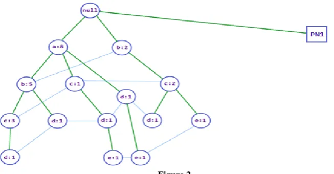
Accuracy is one of the vital parameter in data mining. It refers number of correct predictions over total number of predictions. The higher accuracy indicates the higher stability of the data mining procedure. DME-FP achieved highest accuracy of 92.92% with the average of 91.25%. The nearest accuracy is achieved by MEFP. MEFP gains 89.91% of highest accuracy with the average of 88.89%. Remaining methods Apriori, FP-Growth, Eclat and DFEM are scoring 79.91%, 82.43%, 85.45% and 86.64% of accuracy respectively.

The accuracy report is given in table 5 and compared in Figure 3.

Table 5

Accuracy (%)

Records Apriori FP-Growth Eclat DFEM MEFP DME-FP

10000 80.56 83.59 86.63 87.66 89.69 92.73

20000 80.98 81.24 84.51 85.78 87.37 90.63

30000 79.44 83.96 85.49 85.01 88.53 90.05

40000 80.42 82.12 84.5 87.2 88.58 90.29

50000 79.64 82.12 85.27 85.75 87.9 91.06

60000 79.86 81.76 84.35 87.94 88.85 91.43

70000 78.55 81.56 86.89 87.9 89.91 92.92

80000 79.2 83.96 85.72 85.47 89.23 90.98

90000 80.91 81.61 85.32 87.03 89.73 90.44

37 Figure 3

Table 6

Precision (%)

Records Apriori FP-Growth Eclat DFEM MEFP DME-FP

10000 80.72 83.56 87.08 87.59 89.43 92.95

20000 81.13 81.52 84.23 85.63 87.34 90.73

30000 79.08 84.04 85.01 84.97 88.93 89.89

40000 80.07 82.27 84.15 87.35 88.23 90.12

50000 79.33 81.94 84.9 85.51 87.47 90.76

60000 80.15 81.45 84.45 88.12 88.44 91.42

70000 78.2 81.9 86.59 88.29 89.99 93.37

80000 79.55 84.19 85.5 85.81 89.13 91.44

90000 80.65 81.99 85.03 87.39 89.41 90.77

100000 79.77 82.87 85.65 87.05 88.83 91.92

Precision score determines the reliability of a data mining procedure. Higher precision refers higher reliability. DME-FP achieved highest precision value of 93.37% with precision average of 91.34% whereas MEFP achieved 89.99% of highest precision

with the average of 88.72%. Precision measurement values for proposed method along with existing methods are given in Table 6 and compared in graph given as Figure 4.

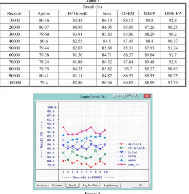
Figure 4 Recall refers the fraction of successfully retrieved relevant items and it is an important parameter in data mining. A good mining procedure should score higher recall values. As per the readings, DME-FP reached 92.8% recall score with 91.22% average

38 Table 7

Recall (%)

Records Apriori FP-Growth Eclat DFEM MEFP DME-FP

10000 80.46 83.45 86.13 88.13 89.8 92.8

20000 80.97 80.95 84.95 85.95 87.26 90.25

30000 79.68 83.91 85.83 85.06 88.29 90.2

40000 80.6 82.55 84.5 87.45 88.4 90.37

50000 79.44 82.07 85.69 85.31 87.93 91.24

60000 79.38 81.36 84.71 88.37 89.04 91.7

70000 78.24 81.88 86.52 87.84 89.48 92.8

80000 79.35 84.25 85.82 85.7 89.27 90.83

90000 80.41 81.11 84.82 86.53 89.55 90.25

100000 79.4 82.88 86.36 86.83 88.99 91.79

Figure 5

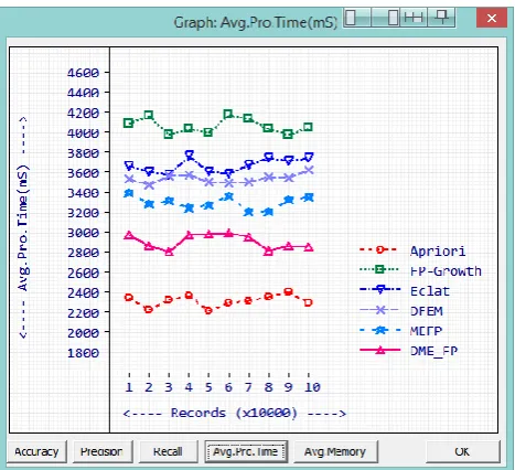
Processing time of a data mining procedure is also a parameter that determines the quality. A good data mining procedure has to produce results with a reasonable time. DME-FP consumed 2918mS of average processing time to process a data block. Apriori consumes the least time of 2324mS average processing time which is lesser than DME-FP. FP-Growth, Eclat, DFEM and MEFP consumed 4072mS, 3677mS, 3548ms and 3306mS

respectively. While comparing other methods excluding Apriori, DME-FP consumed lesser time. With the betterment in other parameters the 594mS time delay can be compromised. Complete processing time readings for all methods are given in Table 8. A comparison graph of processing times is given in Figure 6.

Average Processing Time (mS)

Records Apriori FP-Growth Eclat DFEM MEFP DME-FP

10000 2353 4096 3672 3549 3400 2987

20000 2230 4174 3618 3483 3295 2870

30000 2338 3984 3583 3575 3329 2819

40000 2370 4049 3773 3584 3251 2986

50000 2228 4003 3610 3518 3281 2991

60000 2308 4185 3591 3509 3374 3003

70000 2324 4147 3683 3519 3210 2969

80000 2369 4040 3756 3560 3219 2826

90000 2414 3989 3729 3557 3332 2870

39 Table 8

Figure 6

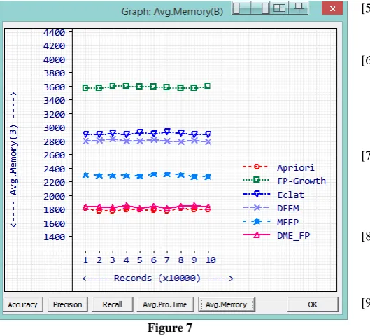
Memory is one of the important computational resources. More memory consumption affects the stability of data mining procedures. While handling large number of item sets and transaction history, consuming more memory will slow down the process. DME-FP consumed 1844 Bytes to process a data

block. The nearest performance method MEFP consumed 2304 Bytes. Apriori consumed the least average memory of 1802 Bytes. Average memory consumption to process a data block by all the methods are recorded in table 9. Memory comparison chart is given in Figure 7.

Table 9

Memory (B)

Records Apriori FP-Growth Eclat DFEM MEFP DME-FP

10000 1821 3586 2902 2817 2312 1846

20000 1781 3583 2905 2825 2307 1846

30000 1787 3611 2924 2848 2302 1832

40000 1807 3614 2909 2815 2302 1865

50000 1804 3607 2930 2815 2298 1821

60000 1792 3609 2915 2832 2329 1852

70000 1786 3598 2948 2810 2320 1820

80000 1821 3580 2927 2804 2311 1858

90000 1809 3586 2900 2826 2283 1865

40 Figure 7

6. CONCLUSION

Based on the experimental results DME-FP scored higher in standard data mining parameters of accuracy, precision and recall. The variation in consumption of computational resources like processing time and memory is very lesser to achieve more reliable association rules in proposed DME-FP. The introduction of TPN and RPT results improved performance of proposed DME-FP makes it is more suitable to use in modern data analytical processes.

7. REFERENCES

[1] Chien Chiang Lin, Hsing-Hung Lin, Kun-Chih Huang. TRIZ retrospect and prospect. Systems and Informatics (ICSAI) IEEE November 2016

[2] Jeff Heaton. Comparing dataset characteristics that favor the Apriori, Eclat or FP-Growth frequent itemset mining algorithms. IEEE April 2016

[3] Arkan A.G.AL-Hamodi, Songfeng LU, Yahya

E.A.AL-Salhi. AN ENHANCED FREQUENT PATTERN

GROWTH BASED ON MAPREDUCE FOR MINING ASSOCIATION RULES. International Journal of Data Mining & Knowledge Management Process (IJDKP) March 2016

[4] Dea Delvia Arifin, Shaufiah, Moch.Arif Bijaksana. Enhancing Spam Detection on Mobile Phone Short Message Service (SMS) Performance using FP-Growth and Naive Bayes Classifier. Asia Pacific Conference on Wireless and Mobile (APWiMob). IEEE 2016

[5] Chunkai Zhang, Xudong Zhang, Panbo Tian. An Approximate Approach to Frequent Itemset Mining, Data Science in Cyberspace (DSC). IEEE June 2017

[6] Wan Aezwani Bt Wan Abu Bakar, Zailani B.Abdullah, Md.Yazid B.Md Saman, Masila Bt Abd Jalil, Mustafa B. Man, Tutut Herawan, Abdul Razak Hamdan. Incremental-Eclat Model: An Implementation via Benchmark Case Study. Advances in Machine Learning and Signal Processing. Springer June 2016

[7] Iona Sudheendran, Ganesh Kumar R. A Dynamic Approach for Frequent Pattern Mining Using Database Characteristics. International Journal for Research in Applied Science & Engineering Technology (IJRASET) MAY 2015

[8] Sagar Bhise1, Prof. Sweta Kale, Effieient Algorithms to find Frequent Itemset Using Data Mining, International Research Journal of Engineering and Technology (IRJET) JUNE 2017

[9] Duo Liu, Yi Lin, Po-Chun Huang, Xiao Zhu, Liang Liang. Durable and Energy Efficient In-Memory Frequent Pattern Mining. IEEE Transactions on Computer-Aided Design of Integrated Circuits and Systems, IEEE March 2017

[10]Mukesh Bathre, Vivek Kumar Vaidya, Alok Sahelay. Memory Efficient Frequent Pattern Mining using Transposition of Database. International Journal of Computer Engineering & Technology (IJCET). APRIL 2016

[11]Data Mining Algorithms In R/Frequent Pattern Mining/The FPGrowthAlgorithm,https://en.wikibooks.org/wiki/Data_M ining_Algorithms_In_R/Frequent_Pattern_Mining/The_FP -Growth_Algorithm

[12]Mahito Sugiyama, Karsten M. Borgwardt, Significant Pattern Mining on Continuous Variables. Cornell University Library 2017

[13]Ian H. Witten, Eibe Frank, Mark A. Hall, Christopher J. Pal. Data Mining: Practical machine learning tools and techniques. Fourth Edition

[14]Mahsa Salehi, Christopher Leckie, James C.Bezdek, Tharshan Vaithianathan, Xuyun Zhang. Fast Memory Efficient Local Outlier Detection in Data Streams, IEEE Transactions on Knowledge and Data Engineering, IEEE December 2016

[15]Souleymane Zida, Philippe Fournier-Viger, Jerry Chun-Wei Lin, Cheng-Chun-Wei Wu, Vincent S. Tseng. EFIM: a fast and memory efficient algorithm for high-utility itemset mining. Knowledge and Information Systems. Springer May,2017