Unsupervised Machine Learning for
Networking: Techniques, Applications
and Research Challenges
MUHAMMAD USAMA1, JUNAID QADIR1, AUNN RAZA2,HUNAIN ARIF2, KOK-LIM ALVIN
YAU3,YEHIA ELKHATIB4, AMIR HUSSAIN5,and ALA-AL-FUQAHA.6
1Information Technology University (ITU)-Punjab, Lahore, Pakistan 2
National University of Science and Technology (NUST), Pakistan
3
Sunway University, Malaysia
4
MetaLab, School of Computing and Communication, Lancaster University, UK
5
Edinburgh Napier University, UK
6
Hamad Bin Khalifa University, Qatar
Corresponding author: Muhammad Usama (e-mail: [email protected]).
ABSTRACT While machine learning and artificial intelligence have long been applied in networking research, the bulk of such works has focused on supervised learning. Recently, there has been a rising trend of employing unsupervised machine learning using unstructured raw network data to improve network per-formance and provide services such as traffic engineering, anomaly detection, Internet traffic classification, and quality of service optimization. The interest in applying unsupervised learning techniques in networking emerges from their great success in other fields such as computer vision, natural language processing, speech recognition, and optimal control (e.g., for developing autonomous self-driving cars). Unsupervised learning is interesting since it can unconstrain us from the need for labeled data and manual handcrafted feature engineering thereby facilitating flexible, general, and automated methods of machine learning. The focus of this survey paper is to provide an overview of the applications of unsupervised learning in the domain of networking. We provide a comprehensive survey highlighting the recent advancements in unsupervised learning techniques and describe their applications in various learning tasks in the context of networking. We also provide a discussion on future directions and open research issues, while also identifying potential pitfalls. While a few survey papers focusing on the applications of machine learning in networking have previously been published, a survey of similar scope and breadth is missing in the literature. Through this paper, we advance the state of knowledge by carefully synthesizing the insights from these survey papers while also providing contemporary coverage of recent advances.
INDEX TERMS Machine Learning,Deep Learning,Unsupervised Learning,Computer Networks
I. INTRODUCTION
Networks—such as the Internet and mobile telecom networks—serve the function of the central hub of modern human societies, which the various threads of modern life weave around. With networks becoming increasingly dy-namic, heterogeneous, and complex, the management of such networks has become less amenable to manual administra-tion, and it can benefit from leveraging support from methods for optimization and automated decision-making from the fields of artificial intelligence (AI) and machine learning (ML). Such AI and ML techniques have already transformed multiple fields—e.g., computer vision, natural language pro-cessing (NLP), speech recognition, and optimal control (e.g., for developing autonomous self-driving vehicles)—with the success of these techniques mainly attributed tofirstly,
FIGURE 1. Outline of the paper
in scope by their need for labeled data. With network data becoming increasingly voluminous (with a disproportionate rise in unstructured unlabeled data), there is a groundswell of interest in leveragingunsupervised ML methodsto utilize unlabeled data, in addition to labeled data where available, to optimize network performance [3]. The rising interest in applying unsupervised ML in networking applications also stems from the need to liberate ML applications from restrictive demands of supervised ML. Another reason of em-ploying unsupervised ML in networking is the expensiveness of curating labeled network data at scale, since labeled data may be unavailable and manual annotation is prohibitively inconvenient, in addition, to be outdated quickly (due to the highly dynamic nature of computer networks) [4].
We are already witnessing the failure of human network administrators to manage and monitor all bits and pieces of network [5], and the problem will only exacerbate with further growth in the size of networks with paradigms such as becoming the Internet of things (IoT). An ML-based network management system (NMS) is desirable in such large networks so that faults/bottlenecks/anomalies may be predicted in advance with reasonable accuracy. In this re-gard, networks already have ample amount of untapped data, which can provide us with decision-making insights making networks more efficient and self-adapting. With unsupervised ML, the pipe dream is that every algorithm for adjusting network parameters (be it, TCP congestion window or rerout-ing network traffic durrerout-ing peak time) will optimize itself
in a self-organizing fashion according to the environment and application, user, and network Quality of Service (QoS) requirements and constraints [6]. Unsupervised ML methods, in concert with existing supervised ML methods, can provide a more efficient method that lets a network manage, monitor, and optimize itself while keeping the human administrators in the loop with the provisioning of timely actionable infor-mation.
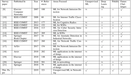
TABLE 1. Comparison of our paper with existing survey and review papers. (Legend:√means covered;×means not covered;≈means partially covered.)
Survey paper
Published In Year # Refer-ences
Areas Focused Unsupervised ML
Deep Learn-ing
Pitfalls Future Chal-lenges [9] Elsevier
Computer Networks
2007 100 ML for Network Intrusion De-tection
≈ × × √
[10] IEEE COMST 2008 68 ML for Internet Traffic Classi-fication
≈ × × ×
[11] IEEE COMST 2013 177 ML for Cognitive Radios ≈ × × ×
[12] IEEE COMST 2014 152 ML for WSNs ≈ × × √
[13] IEEE COMST 2016 113 ML for Cyber Security Intru-sion Detection
≈ × × √
[14] IEEE COMST 2017 269 ML in SONs ≈ × × √
[15] Springer Book Chapter
2017 16 ML for Anomaly Detection in Industrial Networks
≈ × × √
[16] IEEE COMST 2017 260 ML for Network Traffic Con-trol
≈ √ × √
[17] ArXiv 2017 154 ML for Network Intrusion De-tection
≈ √ × ×
[18] Arxiv 2018 282 ML applications in the internet of things
≈ ≈ √ √
[19] Elsevier 2018 148 ML applications in the internet of things
≈ ≈ × ≈
[20] Springer 2018 501 ML in networking √ ≈ × √
[21] Springer 2018 79 ML applications in the internet of things
≈ × × ≈
This Pa-per
- 2019 321 Unsupervised ML in Network-ing
√ √ √ √
learning is a class of machine learning, where hierarchical architectures are used for unsupervised feature learning and these learned features are then used for classification and other related tasks [23]. The versatility of deep learning and distributed ML can be seen in the diversity of their applica-tions that range from self-driving cars to the reconstruction of brain circuits [22]. Unsupervised learning is also often used in conjunction with supervised learning in semi-supervised learning setting to preprocess the data before analysis and thereby help in crafting a good feature representation and in finding patterns and structures in unlabeled data.
The rapid advances in deep neural networks, the democra-tization of enormous computing capabilities through cloud computing and distributed computing, and the ability to store and process large swathes of data have motivated a surging interest in applying unsupervised ML techniques in the networking field. The field of networking also appears to be well suited to, and amenable to applications of un-supervised ML techniques, due to the largely distributed decision-making nature of its protocols, the availability of large amounts of network data, and the urgent need for intelligent/cognitivenetworking. Consider the case of routing in networks. Networks these days have evolved to be very complex, and they incorporate multiple physical paths for redundancy and utilize complex routing methodologies to direct the traffic. The application traffic does not always take the optimal path we would expect, leading to unexpected and inefficient routing performance. To tame such complexity, unsupervised ML techniques can autonomously self-organize the network taking into account a number of factors such as
real-time network congestion statistics as well as application QoS requirements [24].
The purpose of this paper is to highlight the important advances in unsupervised learning, and after providing a tutorial introduction to these techniques, to review how such techniques have been, or could be, used for various tasks in modern next-generation networks comprising both computer networks as well as mobile telecom networks.
appli-cations of unsupervised ML techniques in computer networks and provides readers with a comprehensive discussion of the unsupervised ML trends, as well as the suitability of various unsupervised ML techniques. A tabulated comparison of our paper with other existing survey and review articles is presented in Table 1.
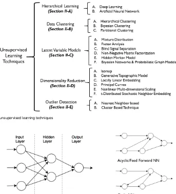
Organization of the paper:The organization of this paper is depicted in Figure 1. Section II provides a discussion on various unsupervised ML techniques (namely, hierarchical learning, data clustering, latent variable models, and outlier detection). Section III presents a survey of theapplications of unsupervised ML specifically in the domain of computer networks. Section IV describes future work and opportuni-ties with respect to the use of unsupervised ML in future networking. Section V discusses a few major pitfalls of the unsupervised ML approach and its models. Finally, Section VI concludes this paper. For the reader’s facilitation, Table 2 shows all the acronyms used in this survey for convenient referencing.
II. TECHNIQUES FOR UNSUPERVISED LEARNING In this section, we will introduce some widely used unsuper-vised learning techniques and their applications in computer networks. We have divided unsupervised learning techniques into six major categories: hierarchical learning, data clus-tering, latent variable models, dimensionality reduction, and outlier detection. Figure 2 depicts a taxonomy of unsuper-vised learning techniques and also the relevant sections in which these techniques are discussed. To provide a bet-ter understanding of the application of unsupervised ML techniques in networking, we have added few subsections highlighting significant applications of unsupervised ML techniques in networking domain.
A. HIERARCHICAL LEARNING
[image:4.576.298.550.80.579.2]Hierarchical learning is defined as learning simple and com-plex features from a hierarchy of multiple linear and non-linear activations. In learning models, a feature is a measur-able property of the input data. Desired features are ideally informative, discriminative, and independent. In statistics, features are also known as explanatory (or independent) vari-ables [26]. Feature learning (also known as data representa-tion learning) is a set of techniques that can learn one or more features from input data [27]. It involves the transformation of raw data into a quantifiable and comparable representation, which is specific to the property of the input but general enough for comparison to similar inputs. Conventionally, features are handcrafted specific to the application on hand. It relies on domain knowledge but even then they do not generalize well to the variation of real-world data, which gives rise to automated learning of generalized features from the underlying structure of the input data. Like other learning algorithms, feature learning is also divided among domains of supervised and unsupervised learning depending on the type of available data. Almost all unsupervised learning algorithms undergo a stage of feature extraction in order to
TABLE 2. List of common acronyms used
ADS Anomaly Detection System
A-NIDS Anomaly & Network Intrusion Detection System AI Artificial Intelligence
ANN Artificial Neural Network ART Adaptive Resonance Theory BSS Blind Signal Separation
BIRCH Balanced Iterative Reducing and Clustering Using Hierarchies CDBN Convolutional Deep Belief Network
CNN Convolutional Neural Network CRN Cognitive Radio Network DBN Deep Belief Network DDoS Distributed Denial of Service
DNN Deep Neural Network DNS Domain Name Service
DPI Deep Packet Inspection EM Expectation-Maximization GTM Generative Topographic Model
GPU Graphics Processing Unit GMM Gaussian Mixture Model HMM Hidden Markov Model
ICA Independent Component Analysis IDS Intrusion Detection System IoT Internet of Things LSTM Long Short-Term Memory
LLE Locally Linear Embedding LRD Low Range Dependencies
ML Machine Learning MLP Multi-Layer Perceptron MDS Multi-Dimensional Scaling MCA Minor Component Analysis NMF Non-Negative Matrix Factorization NMS Network Management System
NN Neural Network
NMDS Nonlinear Multi-dimensional Scaling OSPF Open Shortest Path First
PU Primary User
PCA Principal Component Analysis PGM Probabilistic Graph Model
QoE Quality of Experience QoS Quality of Service
RBM Restricted Boltzmann Machine RNN Recurrent Neural Network SDN Software Defined Network SOM Self-Organizing Map SON Self-Organizing Network SVM Support Vector Machine SON Self Organizing Network SSAE Shrinking Sparse Autoencoder
TCP Transmission Control Protocol
t-SNE t-Distributed Stochastic Neighbor Embedding TL Transfer Learning
VoIP Voice over IP
VoQS Variation of Quality Signature VAE Variational Autoencoder WSN Wireless Sensor Network
learn data representation from unlabeled data and generate a feature vector on the basis of which further tasks are performed.
FIGURE 2. Taxonomy of unsupervised learning techniques
FIGURE 3. Illustration of an ANN (left); Different types of ANN topologies (right)
learning [40] is a hierarchical technique that models high-level abstraction in data using many layers of linear and nonlinear transformations. With deep enough stack of these transformation layers, a machine can self-learn a very com-plex model or representation of data. Learning takes place in hidden layers and the optimal weights and biases of the neurons are updated in two passes, namely, the forward pass and backward pass. A typical ANN and typical cyclic and acyclic topologies of interconnection between neurons are shown in Figure 3. A brief taxonomy of Unsupervised NNs is presented in Figure 4.
An ANN has three types of layers (namely input, hidden and output, each having different activation parameters). Learningis the process of assigning optimal activation pa-rameters enabling ANN to perform input to output map-ping. For a given problem, an ANN may require multiple hidden layers involving a long chain of computations, i.e.,
its depth [41]. Deep learning has revolutionized ML and
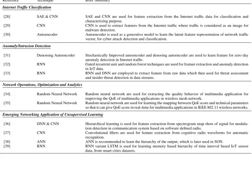
TABLE 3. Applications of hierarchical learning/ deep learning in networking applications
Reference Technique Brief Summary
Internet Traffic Classification
[28] SAE & CNN SAE and CNN are used for feature extraction from the Internet traffic data for classification and characterizing purpose.
[29] CNN CNN is used to extract features from the Internet traffic where traffic is considered as an image for malware detection.
[30] Autoencoder Autoencoder is used as a generative model to learn the latent feature representation of network traffic vector, for cyber attack detection and classification.
Anomaly/Intrusion Detection
[31] Denoising Autoencoder Stochastically Improved autoencoder and denosing autoencoder are used to learn feature for zero day anomaly detection in Internet traffic.
[32] RNN Gated recurrent unit and random forest techniques are used for feature extraction and anomaly detection in IoT data.
[33] RNN RNN and DNN are employed to extract feature from raw data which then used for threat assessment and insider threat detection in data streams.
Network Operations, Optimization and Analytics
[34] Random Neural Network Random neural network are used for extracting the quality behavior of multimedia application for improving the QoE of multimedia applications in wireless mesh network.
[35] Random Neural Network Random neural network are used for learning the mapping between QoE score and technical parameters so that it can give QoE score in real-time for multimedia applications in IEEE 802.11 wireless networks.
Emerging Networking Application of Unsupervised Learning
[36] DNN & CNN Hierarchical learning is used for feature extraction from spectrogram snap shots of signal for modula-tion detecmodula-tion in communicamodula-tion system based on software defined radio.
[37] CNN Convolutional filters are used for feature extraction from cognitive radio waveforms for automatic recognition.
[38] ANN ANN is recommended to learn the hierarchy of the output, which is later used in SON.
[39] RNN RNN variant LSTM is used for learning memory based hierarchy of time interval based IoT sensor data, from smart cities datasets.
[image:6.576.106.466.496.667.2]1) Unsupervised Multilayer Feed Forward NN
Unsupervised multilayer feedforward NN, with reference to graph theory, has a directed graph topology as shown in Fig-ure 3. It consists of no cycles, i.e., does not have a feedback path in input propagation through NN. Such kind of NN is often used to approximate a nonlinear mapping between inputs and required outputs. Autoencoders are the prime examples of unsupervised multilayer feedforward NNs.
a: Autoencoders
An autoencoder is an unsupervised learning algorithm for ANN used to learn compressed and encoded representation of data, mostly for dimensionality reduction and for un-supervised pre-training of feedforward NNs. Autoencoders are generally designed using approximation function and trained using backpropagation and stochastic gradient de-scent (SGD) techniques. Autoencoders are the first of their kind to use the back-propagation algorithm to train with unlabeled data. Autoencoders aim to learn a compact rep-resentation of the function of input using the same number of input and output units with usually less hidden units to encode a feature vector. They learn the input data function by recreating the input at the output, which is called encod-ing/decoding, to learn at the time of training NN. In short, a simple autoencoder learns a low-dimensional representation of the input data by exploiting similar recurring patterns.
Autoencoders have different variants [46] such as vari-ational autoencoders, sparse autoencoders, and denoising autoencoders. Variational autoencoder is an unsupervised learning technique used clustering, dimensionality reduction, and visualization, and for learning complex distributions [47]. In asparse autoencoder, a sparse penalty on the latent layer is applied for extracting a unique statistical feature from unlabeled data. Finally,denoising autoencoders are used to learn the mapping of a corrupted data point to its original location in the data space in an unsupervised manner for manifold learning and reconstruction distribution learning.
2) Unsupervised Competitive Learning NN
Unsupervised competitive learning NNs is a winner-take-all neuron scheme, where each neuron competes for the right of the response to a subset of the input data. This scheme is used to remove the redundancies from the unstructured data. Two major techniques of unsupervised competitive learning NNs are self-organizing maps and adaptive resonance theory NNs.
Self-Organizing/ Kohonen Maps: Self-Organizing Maps
(SOM), also known as Kohonen’s maps [48] [49], are a spe-cial class of NNs that uses the concept ofcompetitive learn-ing, in which output neurons compete amongst themselves to be activated in a real-valued output, results having only single neuron (or group of neurons), calledwinning neuron. This is achieved by creating lateral inhibition connections (negative feedback paths) between neurons [50]. In this orientation, the network determines the winning neuron within several iterations; subsequently, it is forced to reorganize itself based on the input data distribution (hence they are called
Self-Organizing Maps). They were initially inspired by the hu-man brain, which has specialized regions in which different sensory inputs are represented/processed by topologically ordered computational maps. In SOM, neurons are arranged on vertices of a lattice (commonly one or two dimensions). The network is forced to represent higher-dimensional data in lower-dimensional representation by preserving the topolog-ical properties of input data by using neighborhood function while transforming the input into a topological space in which neuron positions in the space are representatives of intrinsic statistical features that tell us about the inherently nonlinear nature of SOMs.
Training a network comprising SOM is essentially a three-stage process after random initialization of weighted connec-tions. The three stages are as follow [51].
• Competition:Each neuron in the network computes its
value using a discriminant function, which provides the basis of competition among the neurons. Neuron with the largest discriminant value in the competition group is declared the winner.
• Cooperation:The winner neuron then locates the center of the topological neighborhood of excited neurons in the previous stage, providing a basis for cooperation among excited neighboring neurons.
• Adaption: The excited neurons in the neighborhood
increase/decrease their individual values of the discrimi-nant function in regard to input data distribution through subtle adjustments such that the response of the winning neuron is enhanced for similar subsequent input. Adap-tion stage is distinguishable into two sub-stages: (1) theordering or self-organizing phase, in which weight vectors are reordered according to topological space; and (2) the convergence phase, in which the map is fine-tuned and declared accurate to provide statistical quantification of the input space. This is the phase in which the map is declared to be converged and hence trained.
One essential requirement in training a SOM is the redun-dancy of the input data to learn about the underlying structure of neuron activation patterns. Moreover, sufficient quantity of data is required for creating distinguishable clusters; withstanding enough data for classification problem, there exist a problem of gray area between clusters and creation of infinitely small clusters where input data has minimal patterns.
mod-els is that they lose old information (updating/diminishing weights) as new information arrives, therefore an ideal model should be flexible enough to accommodate new information without losing the old one, and this is called the plasticity-stability problem. ART models provide a solution to this problem by self-organizing in real time and creating a com-petitive environment for neurons, automatically discriminat-ing/creating new clusters among neurons to accommodate any new information.
ART model resonates around (top-down) observer expec-tations and (bottom-up) sensory information while keeping their difference within the threshold limits of vigilance pa-rameter, which in result is considered as the member of the expected class of neurons [52]. Learning of an ART model primarily consists of a comparison field, recognition field, vigilance (threshold) parameter, and a reset module. The comparison field takes an input vector, which in result is passed, to best match in the recognition field; the best match is the current winning neuron. Each neuron in the recognition field passes a negative output in proportion to the quality of the match, which inhibits other outputs, therefore, exhibiting lateral inhibitions (competitions). Once the winning neuron is selected after a competition with the best match to the input vector, the reset module compares the quality of the match to the vigilance threshold. If the winning neuron is within the threshold, it is selected as the output, else the winning neuron is reset and the process is started again to find the next best match to the input vector. In case where no neuron is capable to pass the threshold test, a search procedure begins in which the reset module disables recognition neurons one at a time to find a correct match whose weight can be adjusted to accom-modate the new match, therefore ART models are called self-organizing and can deal with the plasticity/stability dilemma.
3) Unsupervised Deep NN
In recent years unsupervised deep NN has become the most successful unsupervised structure due to its application in many benchmarking problems and applications [53]. Three major types of unsupervised deep NNs are deep belief NNs, deep autoencoders, and convolutional NNs.
Deep Belief NN: Deep Belief Neural Network or simply Deep Belief Networks (DBN) is a probability-based genera-tive graph model that is composed of hierarchical layers of stochastic latent variables having binary valued activations, which are referred as hidden units or feature detectors. The top layers in DBNs have undirected, symmetric connections between them forming an associative memory. DBNs provide a breakthrough in unsupervised learning paradigm. In the learning stage, DBN learns to reconstruct its input, each layer acting as feature detectors. DBN can be trained by greedy layer-wise training starting from the top layer with raw input, subsequent layers are trained with the input data from the previously visible layer [43]. Once the network is trained in an unsupervised manner and learned the distribution of the data, it can be fine-tuned using supervised learning methods,
or supervised layers can be concatenated in order to achieve the desired task (for instance, classification).
Deep Autoencoder: Another famous type of DBN is the
deep autoencoder, which is composed of two symmetric
DBNs—the first of which is used to encode the input vector, while the second decodes. By the end of the training of the deep autoencoder, it tends to reconstruct the input vector at the output neurons, and therefore the central layer between both DBNs is the actual compressed feature vector.
Convolutional NN: Convolutional NN (CNN) are feed
forward NN in which neurons are adapted to respond to overlapping regions in two-dimensional input fields such as visual or audio input. It is commonly achieved by local sparse connections among successive layers and tied shared weights followed by rectifying and pooling layers which results in transformation invariant feature extraction. Another advantage of CNN over simple multilayer NN is that it is comparatively easier to train due to sparsely connected layers with the same number of hidden units. CNN represents the most significant type of architecture for computer vision as they solve two challenges with the conventional NNs: 1) scalable and computationally tractable algorithms are needed for processing high-dimensional images; and 2) algorithms should be transformation invariant since objects in an image can occur at an arbitrary position. However, most CNN’s are composed of supervised feature detectors in the lower and middle hidden layers. In order to extract features in an unsupervised manner, a hybrid of CNN and DBN, called Convolutional Deep Belief Network (CDBN), is proposed in [54]. Making probabilistic max-pooling1 to cover larger input area and convolution as an inference algorithm makes this model scalable with higher dimensional input. Learning is processed in an unsupervised manner as proposed in [44], i.e., greedy layer-wise (lower to higher) training with unla-beled data.
CDBN is a promising scalable generative model for learn-ing translation invariant hierarchical representation from any high-dimensional unlabeled data in an unsupervised manner taking advantage of both worlds, i.e., DBN and CNN. CNN, being widely employed for computer vision applications, can be employed in computer networks for optimization of Quality of Experience (QoE) and Quality of Service (QoS) of multimedia content delivery over networks, which is an open research problem for next-generation computer networks [55].
4) Unsupervised Recurrent NN
Recurrent NN (RNN) is the most complex type of NN, and hence the nearest match to an actual human brain that processes sequential inputs. It can learn temporal behaviors of a given training data. RNN employs an internal memory per neuron to process such sequential inputs in order to
1Max-pooling is an algorithm of selecting the most responsive receptive
FIGURE 5. Clustering process
exhibit the effect of the previous event on the next. Compared to feed forward NNs, RNN is a stateful network. It may contain computational cycles among states and uses time as the parameter in the transition function from one unit to another. Being complex and recently developed, it is an open research problem to create domain-specific RNN models and train them with sequential data. Specifically, there are two perspectives of RNN to be discussed in the scope of this survey, namely, the depth of the architecture and the training of the network. The depth, in the case of a simple artificial NN, is the presence of hierarchical nonlinear intermediate layers between the input and output signals. In the case of an RNN, there are different hypotheses explaining the concept of depth. One hypothesis suggests that RNNs are inherently deep in nature when expanded with respect to sequential input; there are a series of nonlinear computations between the input at timet(i)and the output at timet(i+k).
However, at an individual discrete time step, certain tran-sitions are neither deep nor nonlinear. There exist input-to-hidden, hidden-to-input-to-hidden, and hidden-to-output transitions, which are shallow in the sense that there are no intermediate nonlinear layers at discrete time step. In this regard, different deep architectures are proposed in [56] that introduce inter-mediate nonlinear transitional layers in between the input, hidden and output layers. Another novel approach is also proposed by stacking hidden units to create a hierarchical representation of hidden units, which mimic the deep nature of standard deep NNs.
Due to the inherently complex nature of RNN, to the best of our knowledge, there is no widely adopted approach for training RNNs and many novel methods (both supervised and unsupervised) are introduced to train RNNs. Considering unsupervised learning of RNN in the scope of this paper, [57] employ Long Short-term Memory (LSTM) RNN to be trained in an unsupervised manner using unsupervised learning algorithms, namely Binary Information Gain Opti-mization and non parametric Entropy OptiOpti-mization, in order to make a network to discriminate between a set of temporal sequences and cluster them into groups. Results have shown remarkable ability of RNNs for learning temporal sequences and clustering them based on a variety of features. Two major types of unsupervised recurrent NN are Hopfield NN and Boltzmann machine.
Hopfield NN: Hopfield NN is a cyclic recurrent NN where each node is connected to others. Hopfield NN provides an abstraction of circular shift register memory with nonlinear activation functions to form a global energy function with guaranteed convergence to local minima. Hopfield NNs are used for finding clusters in the data without a supervisor.
Boltzmann Machine: The Boltzmann machine is a stochas-tic symmetric recurrent NN that is used for search and learn-ing problems. Due to binary vector based simple learnlearn-ing algorithm of Boltzmann machine, very interesting features representing the complex unstructured data can be learned [58]. Since the Boltzmann machine uses multiple hidden lay-ers as feature detectors, the learning algorithm becomes very slow. To avoid slow learning and to achieve faster feature detection instead of Boltzmann machine, a faster version, namely the restricted Boltzmann machine (RBM), is used for practical problems [59]. Restricted Boltzmann machine learns a probability distribution over its input data but since it is restricted in its layer to layer connectivity RBM loses its property of recurrence. It is faster than a Boltzmann machine because it only uses one hidden layer as a feature detector layer. RBM is used for dimensionality reduction, clustering and feature learning in computer networks.
5) Significant Applications of Hierarchical Learning in Networks
which a hybrid model of ART and RNN is employed to learn and predict traffic volume in a computer network in real time. Real-time prediction is essential to adaptive flow control, which is achieved by using hybrid techniques so that ART can learn new input patterns without re-training the entire network and can predict accurately in the time series of RNN. Furthermore, DNNs are also being used in resource allocation and QoE/QoS optimizations. Using NN for optimization, efficient resource allocation without affecting the user experience can be crucial in the time when resources are scarce. Authors of [62], [63] propose a simple DBN for optimizing multimedia content delivery over wireless networks by keeping QoE optimal for end users. Table 3 also provides a tabulated description of hierarchical learning in networking applications. However, these are just a few notable examples of deep learning and neural networks in networks, refer to Section III for more applications and detailed discussion on deep learning and neural networks in computer networks.
B. DATA CLUSTERING
Clustering is an unsupervised learning task that aims to find hidden patterns in unlabeled input data in the form of clusters [64]. Simply put, it encompasses the arrangement of data in meaningful natural groupings on the basis of the similarity between different features (as illustrated in Figure 5) to learn about its structure. Clustering involves the organization of data in such a way that there are high intra-cluster and low inter-cluster similarity. The resulting structured data is termed asdata-concept[65]. Clustering is used in numerous applications from the fields of ML, data mining, network analysis, pattern recognition, and computer vision. The various techniques used for data clustering are described in more detail later in Section II-B. In networking, clustering techniques are widely deployed for applications such as traffic analysis and anomaly detection in all kinds of networks (e.g., wireless sensor networks and mobile ad-hoc networks), with anomaly detection [66].
Clustering improves performance in various applications. McGregor et al. [67] propose an efficient packet tracing approach using the Expectation-Maximization (EM) proba-bilistic clustering algorithm, which groups flows (packets) into a small number of clusters, where the goal is to analyze network traffic using a set of representative clusters.
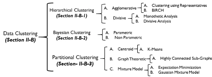
A brief overview of different types of clustering methods and their relationships can be seen in Figure 6. Clustering can be divided into three main types [68], namely hierarchical clustering, Bayesian clustering, and partitional clustering. Hierarchical clustering creates a hierarchical decomposition of data, whereas Bayesian clustering forms a probabilistic model of the data that decides the fate of a new test point probabilistically. In contrast, partitional clustering constructs multiple partitions and evaluates them on the basis of certain criterion or characteristic such as the Euclidean distance.
Before delving into the general sub-types of clustering, there are two unique clustering techniques, which need to be
discussed, namely density-based clustering andgrid-based clustering. In some cases, density-based clustering is classi-fied as a partitional clustering technique; however, we have kept it separate considering its applications in networking. Density-based models target the most densely populated area of data space and separate it from areas having low densities, thus forming clusters [69]. [70] use density-based clustering to cluster data stream in real time, which is important in many applications (e.g., intrusion detection in networks). Another technique is grid-based clustering, which divides the data space into cells to form a grid-like structure; subsequently, all clustering actions are performed on this grid [71]. [71] also present a novel approach that uses a customized grid-based clustering algorithm to detect anomalies in networks. [72] proposed a novel method for clustering the time series data, this scheme was based on a distance measure between temporal features of the time series.
We move on next to describe three major types of data clustering approaches as per the taxonomy is shown in Figure 6.
1) Hierarchical Clustering
Hierarchical clustering is a well-known strategy in data min-ing and statistical analysis in which data is clustered into a hierarchy of clusters using an agglomerative (bottom-up) or a divisive (top-down) approach. Almost all hierarchical clustering algorithms are unsupervised and deterministic. The primary advantage of hierarchical clustering over un-supervised K-means and EM algorithms is that it does not require the number of clusters to be specified beforehand. However, this advantage comes at the cost of computational efficiency. Common hierarchical clustering algorithms have at least quadratic computational complexity compared to the linear complexity of K-means and EM algorithms. Hierarchi-cal clustering methods have a pitfall: these methods fail to ac-curately classify messy high-dimensional data as its heuristic may fail due to the structural imperfections of empirical data. Furthermore, the computational complexity of the common agglomerative hierarchical algorithms is NP-hard. SOM, as discussed in Section II-A2, is a modern approach that can overcome the shortcomings of hierarchical models [73].
2) Bayesian Clustering
FIGURE 6. Clustering taxonomy
data. [75] performed Bayesian non-parametric clustering of network traffic data to determine the network application type.
3) Partitional Clustering
Partitional clustering corresponds to a special class of clus-tering algorithms that decomposes data into a set of disjoint clusters. Givennobservations, the clustering algorithm par-titions a data intok < nclusters [76]. Partitional clustering is further classified into K-means clustering and mixture models.
a: K-Means Clustering
K-means clustering is a simple, yet widely used approach for classification. It takes a statistical vector as an input to de-duce classification models or classifiers. K-means clustering tends to distributemobservations intonclusters where each observation belongs to the nearest cluster. The membership of observation to a cluster is determined using the cluster mean. K-means clustering is used in numerous applications in the domains of network analysis and traffic classification. [77] used K-means clustering in conjunction with supervised ID3 decision tree learning models to detect anomalies in a network. An ID3 decision tree is an iterative supervised decision tree algorithm based on the concept learning system. K-means clustering provided excellent results when used in traffic classification. [78] showed that K-means clustering performs well in traffic classification with an accuracy of 90%.
K-means clustering is also used in the domain of network security and intrusion detection. [79] proposed a K-means algorithm for intrusion detection. Experimental results on a subset of KDD-99 dataset shows that the detection rate stays above 96% while the false alarm rate stays below 4%. Results and analysis of experiments on K-means algorithm have demonstrated a better ability to search clusters globally. Another variation of K-means is known as K-medoids, in which rather than taking the mean of the clusters, the most centrally located data point of a cluster is considered as the reference point of the corresponding cluster [80]. Few of
the applications of K-medoids in the spectrum of anomaly detection can be seen here [80] [81].
b: Mixture Models
Mixture models are powerful probabilistic models for uni-variate and multiuni-variate data. Mixture models are used to make statistical inferences and deductions about the prop-erties of the sub-populations given only observations on the pooled population. They have also used to statistically model data in the domains of pattern recognition, computer vision, ML, etc. Finite mixtures, which are a basic type of mixture model, naturally model observations that are pro-duced by a set of alternative random sources. Inferring and deducing different parameters from these sources based on their respective observations lead to clustering of the set of observations. This approach to clustering tackles drawbacks of heuristic-based clustering methods, and hence it is proven to be an efficient method for node classification in any large-scale network and has shown to yield effective results com-pared to techniques commonly used. For instance, K-means and hierarchical agglomerative methods rely on supervised design decisions, such as the number of clusters or validity of models [82]. Moreover, combining the EM algorithm with mixture models produces remarkable results in deciphering the structure and topology of the vertices connected through a multi-dimensional network [83]. [84] used Gaussian mix-ture model (GMM) to outperform signamix-ture based anomaly detection in network traffic data.
4) Significant Applications of Clustering in Networks
Sup-port Vector Machine (SVM). This hierarchical clustering approach stores abstracted data points instead of the whole dataset, thus giving more accurate and quick classification compared to all past methods, producing better results in detecting anomalies. Another approach [71] discusses the use of grid-based and density-based clustering for anomaly and intrusion detection using unsupervised learning. [86] used k-shape clustering scheme for analyzing spatiotemporal heterogeneity in mobile usage. Basically, a scalable parallel framework for clustering large datasets with high dimensions is proposed and then improved by inculcating frequency pattern trees. Table 4 also provides a tabulated description of data clustering applications in networks. These are just a few notable examples of clustering approaches in networks: refer to Section III for the detailed discussion on some salient clustering applications in the context of networks.
C. LATENT VARIABLE MODELS
A latent variable model is a statistical model that relates the manifest variables with a set of latent or hidden vari-ables. Latent variable model allows us to express relatively complex distributions in terms of tractable joint distributions over an expanded variable space [95]. Underlying variables of a process are represented in higher dimensional space using a fixed transformation, and stochastic variations are known as latent variable models where the distribution in higher dimension is due to small number of hidden variables acting in a combination [96]. These models are used for data visualization, dimensionality reduction, optimization, distribution learning, blind signal separation and factor anal-ysis. Next we will begin our discussion on various latent variable models, namelymixture distribution,factor analysis, blind signal separation, non-negative matrix factorization, Bayesian networks & probabilistic graph models (PGM),
hidden Markov model (HMM), andnonlinear
dimensional-ity reduction techniques (which further includesgenerative topographic mapping, multi-dimensional scaling,principal curves,Isomap,localliy linear embedding, andt-distributed stochastic neighbor embedding).
1) Mixture Distribution
Mixture distribution is an important latent variable model that is used for estimating the underlying density function. Mixture distribution provides a general framework for den-sity estimation by using the simpler parametric distributions. Expectation maximization (EM) algorithm is used for esti-mating the mixture distribution model [97], through max-imization of the log-likelihood of the mixture distribution model.
2) Factor Analysis
Another important type of latent variable model is factor analysis, which is a density estimation model. It has been used quite often in collaborative filtering and dimensionality reduction. It is different from other latent variable models
in terms of the allowed variance for different dimensions as most latent variable models for dimensionality reduction in conventional settings use a fixed variance Gaussian noise model. In the factor analysis model, latent variables have diagonal covariance rather than isotropic covariance.
3) Blind Signal Separation
Blind Signal Separation (BSS), also referred to as Blind Source Separation, is the identification and separation of independent source signals from mixed input signals without or very little information about the mixing process. Figure 7 depicts the basic BSS process in which source signals are extracted from a mixture of signals. It is a fundamental and challenging problem in the domain of signal processing although the concept is extensively used in all types of multi-dimensional data processing. Most common techniques em-ployed for BSS are principal component analysis (PCA) and independent component analysis (ICA).
a) Principal Component Analysis (PCA) is a statistical procedure that utilizes orthogonal transformation on the data to convert n number of possibly correlated variables into lesser k number of uncorrelated variables named principal components. Principal components are arranged in the de-scending order of their variability, first one catering for the most variable and the last one for the least. Being a primary technique for exploratory data analysis, PCA takes a cloud of data in n dimensions and rotates it such that maximum variability in the data is visible. Using this technique, it brings out the strong patterns in the dataset so that these patterns are more recognizable thereby making the data easier to explore and visualize.
PCA has primarily been used for dimensionality reduction in which input data of n dimensions is reduced to k di-mensions without losing critical information in the data. The choice of the number of principal components is a question of the design decision. Much research has been conducted on selecting the number of components such as cross-validation approximations [98]. Optimally, k is chosen such that the ratio of the average squared projection error to the total variation in the data is less than or equal to 1% by which 99% of the variance is retained in thekprincipal components. But, depending on the application domain, different designs can increase/decrease the ratio while maximizing the required output. Commonly, many features of a dataset are often highly correlated; hence, PCA results in retaining 99% of the variance while significantly reducing the data dimensions.
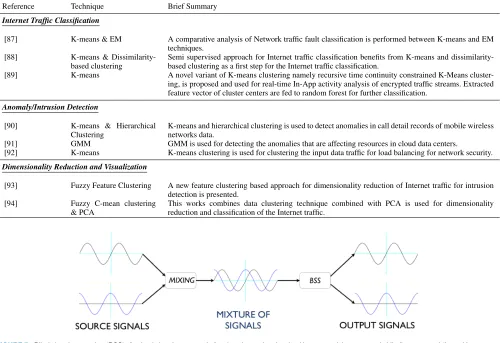
de-TABLE 4. Applications of data clustering in networking applications
Reference Technique Brief Summary
Internet Traffic Classification
[87] K-means & EM A comparative analysis of Network traffic fault classification is performed between K-means and EM techniques.
[88] K-means & Dissimilarity-based clustering
Semi supervised approach for Internet traffic classification benefits from K-means and dissimilarity-based clustering as a first step for the Internet traffic classification.
[89] K-means A novel variant of K-means clustering namely recursive time continuity constrained K-Means cluster-ing, is proposed and used for real-time In-App activity analysis of encrypted traffic streams. Extracted feature vector of cluster centers are fed to random forest for further classification.
Anomaly/Intrusion Detection
[90] K-means & Hierarchical Clustering
K-means and hierarchical clustering is used to detect anomalies in call detail records of mobile wireless networks data.
[91] GMM GMM is used for detecting the anomalies that are affecting resources in cloud data centers.
[92] K-means K-means clustering is used for clustering the input data traffic for load balancing for network security.
Dimensionality Reduction and Visualization
[93] Fuzzy Feature Clustering A new feature clustering based approach for dimensionality reduction of Internet traffic for intrusion detection is presented.
[94] Fuzzy C-mean clustering & PCA
[image:13.576.36.544.78.417.2]This works combines data clustering technique combined with PCA is used for dimensionality reduction and classification of the Internet traffic.
FIGURE 7. Blind signal separation (BSS): A mixed signal composed of various input signals mixed by some mixing process is blindly processed (i.e., with no or minimal information about the mixing process) to show the original signals.
pendence or maximizing the non-Gaussian property among the components in the input signals by keeping the under-lying assumptions valid. Statistically, ICA can be seen as the extension of PCA, while PCA tries to maximize the second moment (variance) of data, hence relying heavily on Gaussian features; on the other hand, ICA exploits inherently non-Gaussian features of the data and tries to maximize the fourth moment of linear combination of inputs to extract non-normal source components in the data [99].
4) Non-Negative Matrix Factorization
Non-Negative Matrix Factorization (NMF) is a technique to factorize a large matrix into two or more smaller matrices with no negative values, that is when multiplied, it recon-structs the approximate original matrix. NMF is a novel method in decomposing multivariate data making it easy and straightforward for exploratory analysis. By NMF, hidden patterns and intrinsic features within the data can be iden-tified by decomposing them into smaller chunks, enhanc-ing the interpretability of data for analysis, with positivity constraints. However, there exist many classes of algorithms
[100] for NMF having different generalization properties, for example, two of them are analyzed in [101], one of which minimizes the least square error and while the other focuses on the Kullback-Leibler divergence keeping algorithm con-vergence intact.
5) Hidden Markov Model
[image:13.576.40.543.83.426.2]6) Bayesian Networks & Probabilistic Graph Models (PGM)
In Bayesian learning we try to find the posterior probability distributions for all parameter settings, in this setup, we ensure that we have a posterior probability for every possible parameter setting. It is computationally expensive but we can use complicated models with a small dataset and still avoid overfitting. Posterior probabilities are calculated by dividing the product of sampling distribution and prior distribution by marginal likelihood; in simple words, posterior probabilities are calculated using Bayes theorem. The basis of reinforce-ment learning was also derived by using Bayes theorem [102]. Since Bayesian learning is computationally expensive a new research trend is approximate Bayesian learning [103]. Authors in [104] have given a comprehensive survey of different approximate Bayesian inference algorithms. With the emergence of Bayesian deep learning framework the deployment of Bayes learning based solution is increasing rapidly.
Probabilistic graph modeling is a concept associated with Bayesian learning. A model representing the probabilistic relationship between random variables through a graph is known as a probabilistic graph model (PGM). Nodes and edges in the graph represent a random variable and their prob-abilistic dependence, respectively. PGM are of two types: directed PGM and undirected PGM. Bayes networks also fall in the regime of directed PGM. PGM is used in many important areas such as computer vision, speech processing, and communication systems. Bayesian learning combined with PGM and latent variable models forms a probabilistic framework where deep learning is used as a substrate for making improved learning architecture for recommender sys-tems, topic modeling, and control systems [105].
7) Significant Applications of Latent Variable Models in Networks
In [106], authors have applied latent structure on email cor-pus to find interpretable latent structure as well as evaluating its predictive accuracy on missing data task. A dynamic latent model for a social network is represented in [107]. Characterization of the end-to-end delay using a Weibull mixture model is discussed in [108]. Mixture models for end host traffic analysis have been explored in [109]. BSS is a set of statistical algorithms that are widely used in differ-ent application domains to perform differdiffer-ent tasks such as dimensionality reduction, correlating and mapping features, etc. [110] employed PCA for Internet traffic classification in order to separate different types of flows in a network packet stream. Similarly, authors of [111] used a semi-supervised approach, where PCA is used for feature learning and an SVM classifier for intrusion detection in an autonomous net-work system. Another approach for detecting anomalies and intrusions proposed in [112] uses NMF to factorize different flow features and cluster them accordingly. Furthermore, ICA has been widely used in telecommunication networks to separate mixed and noisy source signals for efficient service. For example, [113] extends a variant of ICA called Efficient
Fast ICA (EF-ICA) for detecting and estimating the symbol signals from the mixed CDMA signals received from the source endpoint.
In other literature, PCA uses a probabilistic approach to find the degree of confidence in detecting an anomaly in wireless networks [114]. Furthermore, PCA is also chosen as a method of clustering and designing Wireless Sensor Networks (WSNs) with multiple sink nodes [115]. However, these are just a few notable examples of BSS in networks, refer to Section III for more applications and detailed discus-sion on BSS techniques in the networking domain.
Bayesian learning has been applied for classifying Internet traffic, where Internet traffic is classified based on the poste-rior probability distributions. For early traffic identification in campus network real discretized conditional probability has been used to construct a Bayesian classifier [116]. Host-level intrusion detection using Bayesian networks is proposed in [117]. Authors in [118] purposed a Bayesian learning based feature vector selection for anomalies classification in BGP. Port scan attacks prevention scheme using a Bayesian learn-ing approach is discussed in [119]. Internet threat detection estimation system is presented in [120]. A new approach towards outlier detection using Bayesian belief networks is described in [121]. Application of Bayesian networks in MIMO systems has been explored in [122]. Location estima-tion using Bayesian network in LAN is discussed in [123]. Similarly, Bayes theory and PGM are both used in Low-Density Parity Check (LDPC) and Turbo codes, which are the fundamental components of information coding theory. Table 5 also provides a tabulated description of latent variable models applications in networking.
D. DIMENSIONALITY REDUCTION
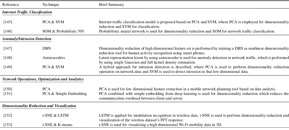
TABLE 5. Applications of latent variable models in networking applications
Reference Technique Brief Summary
Internet Traffic Classification
[124] Mixture Distribution An improved EM algorithm is proposed which derives a better GMM and used for the Internet traffic classification.
[125] PCA PCA based feature selection approach is used for the Internet traffic classification. Where PCA is employed for feature selection and irrelevant feature removal.
[126] NMF NMF based models are applied on the data streams to find the traffic patterns which frequently occurs in network for identification and classification of tidal traffic patterns in metro area mobile network traffic.
Anomaly/Intrusion Detection
[127] Bayesian Networks Bayesian networks are employed for anomaly and intrusion detection such as DDoS attacks in cloud computing networks.
[128] Hidden Semi-Markov Model
Hidden semi-Markov model is used to detect LTE signalling attack.
Network Operations, Optimization and Analytics
[129] Bayesian Networks Scale-able Bayesian network models are used for data flow monitoring and analysis.
[130] HMM HMM and statistical analytic techniques combined with semantic analysis are used to propose a network management tool.
Dimensionality Reduction and Visualization
[131] PCA & Factor Analysis PCA and factor analysis are used for dimensionality reduction and latent correlation identification in mobile traffic demand data.
[132] PCA PCA is used for dimensionality reduction and orthogonal coordinates of the social media profiles in ranking the social media profiles.
considers supervised data labels, while dimensionality reduc-tion focuses on the data points and their distribureduc-tions in an N-dimensional space.
There exist different techniques for reducing data di-mensions [138] including projection of higher dimensional points onto lower dimensions, independent representation, and sparse representation, which should be capable of recon-structing the approximate data. Dimensionality reduction is useful for data modeling, compression, and visualization. By creating representative functional dimensions of the data and eliminating redundant ones, it becomes easier to visualize and form a learning model. Independent representation tries to disconnect the source of variation underlying the data distribution such that the dimensions of the representation are statistically independent [40]. Sparse representation tech-nique represents the data vectors in linear combinations of small basis vectors.
It is worth noting here that many of the latent variable mod-els (e.g., PCA, ICA, factor analysis) also function as tech-niques for dimensionality reduction. In addition to techtech-niques such as PCA, ICA—which infer the latent inherent structure of the data through a linear projection of the data—a number of nonlinear dimensionality reduction techniques have also been developed and will be focused upon in this section to avoid repetition of linear dimensionality reduction techniques that have already been covered as part of the previous subsec-tion. Linear dimensionality reduction techniques are useful in many settings but these methods may miss important nonlin-ear structure in the data due to their subspace assumption,
which posits that the high-dimensional data points lie on a linear subspace (for example, on a 2-D or 3D plane). Such an assumption fails in high dimensions when data points are random but highly correlated with neighbors. In such environments nonlinear dimensionality reductions through
manifold learning techniques—which can be construed as
an attempt to generalize linear frameworks like PCA so that nonlinear structure in data can also be recognized—become desirable. Even though some supervised variants also exist, manifold learning is mostly performed in an unsupervised fashion using the nonlinear manifold substructure learned from the high-dimensional structure of the data from the data itself without the use of any predetermined classifier or labeled data. Some nonlinear dimensionality reduction (manifold learning) techniques are described below:
1) Isomap
Isomap is a nonlinear dimensionality reduction technique that finds the underlying low dimensional geometric infor-mation about a dataset. Algorithmic features of PCA and MDS are combined to learn the low dimensional nonlinear manifold structure in the data [139]. Isomap uses geodesic distance along the shortest path to calculate the low dimen-sion representation shortest path, which can be computed using Dijkstra’s algorithm.
2) Generative Topographic Model
dimen-sional distributions embedded in high dimendimen-sional spaces [140]. Data space in GTM is represented as reference vec-tors and these vecvec-tors are a projection of latent points in data space. It is a probabilistic variant of SOM and works by calculating the Euclidean distance between data points. GTM optimizes the log-likelihood function, and the resulting probability defines the density in data space.
3) Locally Linear Embedding
Locally linear embedding (LLE) [133] is an unsupervised nonlinear dimensionality reduction algorithm. LLE repre-sents data in lower dimensions yet preserving the higher dimensional embedding. LLE depicts data in a single global coordinate of lower dimensional mapping of input data. LLE is used to visualize multi-dimensional dimensional manifolds and feature extraction.
4) Principal Curves
The principal curve is a nonlinear dataset summarizing tech-nique where non-parametric curves pass through the middle of multi-dimensional dataset providing the summary of the dataset [141]. These smooth curves minimize the average squared orthogonal distance between data points, this pro-cess also resembles the maximum likelihood for nonlinear regression in the presence of Gaussian noise [142].
5) Nonlinear Multi-dimensional Scaling
Nonlinear multi-dimensional scaling (NMDS) [143] is a non-linear latent variable representation scheme. It works as an alternative scheme for factor analysis. In factor analysis, a multivariate normal distribution is assumed and similarities between different objects are expressed as a correlation ma-trix. Whereas NMDS does not impose such a condition, and it is designed to reach the optimal low dimensional configu-ration where similarities and dissimilarities among matrices can be observed. NMDS is also used in data visualization and mining tools for depicting the multi-dimensional data in 3 dimensions based on the similarities in the distance matrix.
6) t-Distributed Stochastic Neighbor Embedding
t-distributed stochastic neighbor embedding (t-SNE) is an-other nonlinear dimensionality reduction scheme. It is used to represent high dimensional data in 2 or 3 dimensions. t-SNE constructs a probability distribution in high dimen-sional space and constructs a similar distribution in lower dimensions and minimizes the Kullbackâ ˘A ¸SLeibler (KL) di-vergence between two distributions (which is a useful way to measure the difference between two probability distributions) [144].
Table 6 also provides a tabulated description of dimension-ality reduction applications in networking. The applications of nonlinear dimensionality reduction methods are later de-scribed in detail in Section III-D.
E. OUTLIER DETECTION
Outlier detection is an important application of unsupervised learning. A sample point that is distant from other samples is called an outlier. An outlier may occur due to noise, measurement error, heavy tail distributions and a mixture of two distributions. There are two popular underlying tech-niques for unsupervised outlier detection upon which many algorithms are designed, namely the nearest neighbor based technique and clustering based method.
1) Nearest Neighbor Based Outlier Detection
The nearest neighbor method works on estimating the Eu-clidean distances or average distance of every sample from all other samples in the dataset. There are many algorithms based on nearest neighbor based techniques, with the most famous extension of the nearest neighbor being a k-nearest neighbor technique in which only k nearest neighbors par-ticipate in the outlier detection [154]. Local outlier factor is another outlier detection algorithm, which works as an exten-sion of the k-nearest neighbor algorithm. Connectivity-based outlier factors [155], influenced outlierness [156], and local outlier probability models [157] are few famous examples of the nearest neighbor based techniques.
2) Cluster Based Outlier Detection
Clustering based methods use the conventional K-means clustering technique to find dense locations in the data and then perform density estimation on those clusters. After density estimation, a heuristic is used to classify the formed cluster according to the cluster size. Anomaly score is com-puted by calculating the distance between every point and its cluster head. Local density cluster based outlier factor [158], clustering based multivariate Gaussian outlier score [159] [160] and histogram based outlier score [161] are the famous cluster based outlier detection models in literature. SVM and PCA are also suggested for outlier detection in literature.
3) Significant Applications of Outlier Detection in Networks
Outlier detection algorithms are used in many different appli-cations such as intrusion detection, fraud detection, data leak-age prevention, surveillance, energy consumption anomalies, forensic analysis, critical state detection in designs, elec-trocardiogram and computed tomography scan for tumor detection. Unsupervised anomaly detection is performed by estimating the distances and densities of the provided non-annotated data [162]. More applications of outlier detection schemes will be discussed in Section III
F. LESSONS LEARNT
Key lessons drawn from the review of unsupervised learning techniques are summarized below.
TABLE 6. Applications of dimensionality reduction in networking applications
Reference Technique Brief Summary
Internet Traffic Classification
[145] PCA & SVM Internet traffic classification model is proposed based on PCA and SVM, where PCA is employed for dimensionality reduction and SVM for classification.
[146] SOM & Probabilistic NN Probabilistic neural network is used for dimensionality reduction and SOM for network traffic classification.
Anomaly/Intrusion Detection
[147] DBN Dimensionality reduction of high dimensional feature set is performed by training a DBN as nonlinear dimensionality reduction tool for human activity recognition using smart phones.
[148] Autoencoders Latent representation learnt by using autoencoder is used for anomaly detection in network traffic, which is performed by using single Gaussian and full kernel density estimation.
[149] PCA & SVM A hybrid approach for intrusion detection is described, where PCA is used to perform dimensionality reduction operation on network data and SVM is used to detect intrusion in that low dimensional data.
Network Operations, Optimization and Analytics
[150] PCA PCA is used for low dimensional feature extraction in a mobile network planning tool based on data analytic. [151] PCA & Simple Embedding PCA combined with simple embedding from deep learning is used for dimensionality reduction which reduces the
communication overhead between client and server.
Dimensionality Reduction and Visualization
[152] t-SNE & LSTM LSTM is applied for modulation recognition in wireless data. t-SNE is used to perform dimensionality reduction and visualization of the wireless dataset’s FFT response.
[153] t-SNE & K-means t-SNE is used for visualizing a high dimensional Wi-Fi mobility data in 3D.
2) Learning the joint distribution of a complex distribu-tion over an expanded variable space is a difficult task. Latent variable models have been the recommended and well-established schemes in literature for this prob-lem. These models are also used for dimensionality reduction and better representation of data.
3) Visualization of unlabeled multidimensional data is another unsupervised task. In this research, we have explored the dimensionality reduction as an underlying scheme for developing better multidimensional data visualization tools.
III. APPLICATIONS OF UNSUPERVISED LEARNING IN NETWORKING
In this section, we will introduce some significant appli-cations of the unsupervised learning techniques that have been discussed in Section II in the context of computer networks. We highlight the broad spectrum of applications in networking and emphasize the importance of ML-based tech-niques, rather than classical hard-coded statistical methods, for achieving more efficiency, adaptability, and performance enhancement.
A. INTERNET TRAFFIC CLASSIFICATION
Internet traffic classification is of prime importance in net-working as it provides a way to understand, develop and mea-sure the Internet. Internet traffic classification is an important component for service providers to understand the charac-teristics of the service such as quality of service, quality of experience, user behavior, network security and many other key factors related to the overall structure of a network [163]. In this subsection, we will survey the unsupervised learning applications in network traffic classification.
As networks evolve at a rapid pace, malicious intruders are also evolving their strategies. Numerous novel hacking and intrusion techniques are being regularly introduced causing severe financial jolts to companies and headaches to their administrators. Tackling these unknown intrusions through accurate traffic classification on the network edge, therefore, becomes a critical challenge and an important component of the network security domain. Initially, when networks used to be small, simple port-based classification technique that tried to identify the associated application with the corresponding packet based on its port number was used. However, this approach is now obsolete because recent malicious software uses a dynamic port-negotiation mechanism to bypass fire-walls and security applications. A number of contrasting Internet traffic classification techniques have been proposed since then, and some important ones are discussed next.
Most of the modern traffic classification methods use different ML and clustering techniques to produce accurate clusters of packets depending on their applications, thus pro-ducing efficient packet classification [10]. The main purpose of classifying network’s traffic is to recognize the destination application of the corresponding packet and to control the flow of the traffic when needed such as prioritizing one flow over others. Another important aspect of traffic classification is to detect intrusions and malicious attacks or screen out forbidden applications (packets).