Analysis of Influencing Factors on Survival Time of Patients with Heart Failure

ISSN Print: 2161-718X

DOI: 10.4236/ojs.2018.84042 Jul. 19, 2018 651 Open Journal of Statistics

Analysis of Influencing Factors on Survival

Time of Patients with Heart Failure

Jianwei Sheng

1

_{, Xiyuan Qian}

1

_{, Tong Ruan}

2

1_{School of Science, East China University of Science and Technology, Shanghai, China}

2_{School of Information Science and Engineering, East China University of Science and Technology, Shanghai, China}

Abstract

To explore the influencing factors of survival time of patients with heart fail-ure, a total of 1789 patients with heart failure were collected from Shanghai Shuguang Hospital. The Cox proportional hazards model and the mixed ef-fects Cox model were used to analyze the factors on survival time of patients. The results of Cox proportional hazards model showed that age (RR = 1.32), hypertension (RR = 0.67), ARB (RR = 0.55), diuretic (RR = 1.48) and anti-platelet (RR = 0.53) have significant impacts on the survival time of patients. The results of mixed effects Cox model showed that age (RR = 1.16), hyper-tension (RR = 0.61), lung infection (RR = 1.43), ARB (RR = 0.64), β-blockers (RR = 0.77) and antiplatelet (RR = 0.69) have a significant impact on the sur-vival time of patients. The results are consistent with the covariates age, hypertension, ARB and antiplatelet but inconsistent with the covariates lung infection and β-blockers.

Keywords

Heart Failure, Survival Analysis, Longitudinal Data, Mixed Effects Cox Model

1. Introduction

Heart failure is a syndrome with symptoms and signs caused by cardiac dysfunc-tion, resulting in reduced longevity [1]. The prevalence of heart failure in west-ern countries is 1% - 2% of the adult population and 5 - 10 per 1000 population per year, respectively [2][3]. In China, the prevalence of heart failure in Chinese population aged 35 - 74 is 0.9% and the population significantly increases with age [4][5]. With the acceleration of population aging in China, it is foreseeable that the burden caused by heart failure will become heavier in the near future. So it is important to study and analyze the influencing factors of the survival time How to cite this paper: Sheng, J.W., Qian,

X.Y. and Ruan, T. (2018) Analysis of In-fluencing Factors on Survival Time of Pa-tients with Heart Failure. Open Journal of Statistics, 8, 651-659.

https://doi.org/10.4236/ojs.2018.84042

Received: May 6, 2018 Accepted: July 16, 2018 Published: July 19, 2018

Copyright © 2018 by authors and Scientific Research Publishing Inc. This work is licensed under the Creative Commons Attribution International License (CC BY 4.0).

DOI: 10.4236/ojs.2018.84042 652 Open Journal of Statistics

of patients with heart failure.

In medical research, follow-up is the common way to study the law of things; for instance: study the efficacy of a drug, study the survival time after surgery, study the lifetime of a medical device [6][7]. The common ground of the above studies is that it will take some time to trace the research objects, which was called the survival time in statistics. The study of the distribution and influen-cing factors of survival time is the so-called survival analysis [8] [9][10]. Pro-portional hazard regression model has become the most common used proce-dure for modeling the relationship of covariates to a survival or other censored outcome since this model was proposed by D.R. Cox in 1972 [11]. In clinical practice, many studies collect both longitudinal data [12][13](longitudinal data are data in which a response variable is measured at different time points over time) and survival-time data. In this paper, Cox proportional hazards model was used to model the survival-time data and mixed effects Cox model [14][15] was used to model the survival-time and longitudinal data.

2. Models

2.1. Cox Proportional Hazards Model

The Cox proportional hazards model was proposed by British statistician D.R. Cox in 1972, which has been widely applied to analyze the effect of exposure and other covariates on patient’s survival. The Cox model specifies the hazard for in-dividual i as:

( )

0

( )

exp

(

1 1 2 2

)

0

( )

exp

(

( )

)

i t t Xi Xi pXip t X ti

λ

=

λ

β

+

β

+ +_

β

=

λ

β

₍₁₎

where β =

(

β β1, ,2 βp

)

T is a p×1 column vector of coefficients,

(

1, 2, ,

)

i i i ip

X = X X  X is a 1×p vector of covariates for subject i, and λ0

( )

t

is an unspecified nonnegative function of time called the baseline hazard, de-scribing how the risk of event per time unit changes over time at baseline levels of covariates. Since the hazard ratio for two subjects with fixed covariate vectors

i

X and Xj

( )

( )

00

( )

( )

(

(

)

)

(

(

)

)

exp exp exp i i i j j j t X t X X

t t X

λ β

λ

β

λ = λ β = − (2)

is constant over time, the model is called proportional hazards model.

Let the event be observed to have occurred with subject i at time ti. The

probability that happened can be written as

( )

(

₍

)

₎

:

:j i j i

i i i

i j t t i j t t t X L t X λ θ β θ λ ≥ ≥ = =

∑

∑

(3)

where

θ

j =exp

(

Xj

β

)

and the summation is over the set of subjects j who is

still under observation at time ti, the set is called risk set and denoted by R t

( )

i ,

DOI: 10.4236/ojs.2018.84042 653 Open Journal of Statistics

( )

(

₍

)

₎

( ) 1 exp exp i i n i

i _{j R t j}

X PL X δ β β β = _∈     =    

∏

_∑

(4)

where δi is 1 if the event is happened to subject i and 0 otherwise.

2.2. Mixed Effects Cox Model

In clinical practice, some subjects may be observed more than once during the time from first hospitalization to death. The number of hospitalizations and the days between two hospitalizations varies from patient to patient in the heart failure set. The Cox proportional hazards model only uses the survival-time data, which inevitably lose some useful information. The data obtained from multiple measurements of a series of experimental individuals over time are called longi-tudinal data. More precisely, suppose there are m individuals in an experiment where each individual is measured over time. Y Yi1, ,i2 Y iin_i, =1, , m are the

measured data for the individual i at time ti1<ti2<<tini , then

{

Yik:1≤ ≤k ni,1≤ ≤i m

}

is called longitudinal data, which is also called panel

data in econometrics [16]. This type of data is different from cross-section data and time series data. The linear mixed effects model is a common model to dealing with the longitudinal data [17]. It adds individual difference as random effects into the regression model. These random effects describe how every ob-ject’s measurement changes over time and reflect the internal structure of the longitudinal data. In matrix notation a mixed model can be represented as:

( )

T T _{, 0,}

Y X= β+Z b+ε b N∼ Σ (5)

where X and Z are the design matrices for the fixed and random effects re-spectively, β is the vector of fixed-effects coefficients and b is the vector of random effects coefficients and ε is the random error. The random effects dis-tribution is modeled as Gaussian with mean zero and a variance matrix

Σ

. Combining Equation (1) and (3) yields the mixed effects Cox model:

( )

( )

(

T T

)

( )

0 exp , 0,

t t X Z b b N

λ

=

λ

β

+ ∼ Σ ₍₆₎

Coefficients can be estimated based on the partial likelihood:

(

)

₀

( ) ( )

( )

(

( )

)

1

ln , n _{i i} ln _j exp _j d

i j

PL β b ∞ Y t η t Y t η t t

=      = −   _{  }       

∑

∫

∑

(7)

where ηi

( )

t =X ti

( )

β+Z t bi

( )

_{is the linear score for subject} i at time t and

( )

1

i

Y t = if subject i is still under observation at time t and 0 otherwise [18] [19].

3. Data

DOI: 10.4236/ojs.2018.84042 654 Open Journal of Statistics

time out of hospital date or the date of death or the end date of the study. Ac-cording to the guidance of the doctor formed the heart failure dataset used in this paper. This dataset contains data from 1789 patients with heart failure, for a total of 8332 observations and 23 covariates. See Table 1 for details.

Most are categorical variables, but age is a multi-variable. Its distribution is shown in Figure 1.

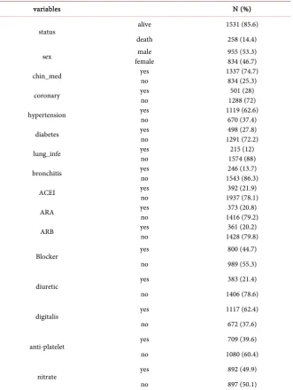
Statistics for other binary variables are shown in Table 2.

4. Results

[image:4.595.198.540.272.738.2]

Firstly, we use the Cox proportional hazards to model the survival-time data with all covariates. The results are shown in Table 3.

Table 1. Variables description in heart failure dataset.

variables Description Data Type

Id Patient id Categorical

num Hospitalization number of patients Categorical Status 1 = dead, 0 = alive Binary

day Number of days between first hospitalization and _{death or last out of hospital} Numeric

days Number of days between first hospitalization and _{this in hospitalization date} Numeric

age 1 = (0,40], 2 = (41,50], 3 =(51,60], 4 = (61,70], _{5 = (71,80], 6 = (81,90], 7 = (91,100]} Multi-category

sex 1 = male, 0 = female Binary Chin_Med Whether used Chinese Medicine? 1 = yes, 0 = no Binary RBC Red blood cells in mg/ml Numeric HGB Hemoglobin in mg/ml Numeric hypertension Presence of hypertension, 1 = yes, 0 = no Binary

coronary Presence of coronary heart disease, 1 = yes, 0 = no Binary diabetes Presence of diabetes, 1 = yes, 0 = no Binary lung_infe Presence of lung infection, 1 = yes, 0 = no Binary bronchitis Presence of chronic bronchitis, 1 = yes, 0 = no Binary

ACEI Whether used angiotensin converting enzyme _{inhibitors? 1 = yes, 0 = no} Binary

ARA Whether used aldosterone receptor antagonists? _{1 = yes, 0 = no} Binary

ARB Whether used angiotensin receptor blocker? _{1 = yes, 0 = no} Binary

[image:5.595.209.541.88.529.2]

DOI: 10.4236/ojs.2018.84042 655 Open Journal of Statistics Table 2. Statistics for binary variable in hear failure set (total = 1789).

variables N (%)

status alive 1531 (85.6)

death 258 (14.4)

sex _female male 955 (53.3) _{834 (46.7)}

chin_med yes _no 1337 (74.7) _{834 (25.3)}

coronary yes _{no 1288 (72)} 501 (28)

hypertension yes _no 1119 (62.6) _{670 (37.4)}

diabetes yes _{no 1291 (72.2)} 498 (27.8)

lung_infe yes _{no 1574 (88)} 215 (12)

bronchitis yes _{no 1543 (86.3)} 246 (13.7)

ACEI yes _{no 1937 (78.1)} 392 (21.9)

ARA yes _{no 1416 (79.2)} 373 (20.8)

ARB yes _{no 1428 (79.8)} 361 (20.2)

Blocker yes 800 (44.7)

no 989 (55.3)

diuretic yes 383 (21.4)

no 1406 (78.6)

digitalis yes 1117 (62.4)

no 672 (37.6)

anti-platelet yes 709 (39.6)

no 1080 (60.4)

nitrate yes 892 (49.9)

no 897 (50.1)

Secondly, we use the mixed effects Cox model to model the survival-time data and longitudinal data with all the covariates and variable day as the covariate for random effects. The results are shown in Table 4.

5. Conclusions

[image:6.595.210.535.81.299.2]

DOI: 10.4236/ojs.2018.84042 656 Open Journal of Statistics Figure 1. Distribution of heart failure patients’ age.

Table 3. Result of Cox proportional hazards model with all covariates.

variables coef RR Se (coef) z p-value sex 0.222649 1.249383 0.178811 1.245 0.21307 age 0.275551 1.317256 0.097916 2.814 0.00489 Chin_med −0.31796 0.727633 0.200295 −1.587 0.11241 RBC −0.1807 0.834684 0.244466 −0.739 0.4598 HGB −0.00859 0.991447 0.007816 −1.099 0.27175 hypertension −0.40512 0.6669 0.196386 −2.063 0.03913 coronary 0.029494 1.029934 0.203818 0.145 0.88494 diabetes −0.01215 0.987926 0.22145 −0.055 0.95625 lung_infe −0.26373 0.768185 0.307327 −0.858 0.39082 bronchitis 0.218949 1.244768 0.21796 1.005 0.31512 ACEI −0.24764 0.780638 0.240374 −1.03 0.3029

ARA −0.27402 0.760313 0.21431 −1.279 0.20102 ARB −0.60086 0.54834 0.266228 −2.257 0.02401 Bblocker −0.19269 0.824737 0.186844 −1.031 0.3024

diuretic 0.389164 1.475747 0.191756 2.029 0.04241 digitalis 0.305065 1.356714 0.184673 1.652 0.09855 anti-platelet −0.64137 0.526573 0.206546 −3.105 0.0019

nitrate 0.319543 1.376498 0.173849 1.838 0.06605

[image:6.595.208.539.353.697.2]

[image:7.595.207.538.88.412.2]

DOI: 10.4236/ojs.2018.84042 657 Open Journal of Statistics Table 4. Results of mixed effects Cox model.

variables coef RR Se (coef) z p-value sex 0.301405 1.351757 0.161594 1.87 0.062 age 0.144165 1.155074 0.067629 2.13 0.033 Chin_med −0.02249 0.977757 0.082878 −0.27 0.79

RBC −0.1126 0.893511 0.169517 −0.66 0.51 HGB −0.01085 0.989209 0.005333 −2.03 0.042 hypertension −0.49125 0.611863 0.127701 −3.85 0.00012

coronary −0.1687 0.844765 0.140132 −1.2 0.23 diabetes −0.23967 0.786885 0.161708 −1.48 0.14 lung_infe 0.356836 1.428802 0.124253 2.87 0.0041 bronchitis 0.250458 1.284613 0.148653 1.68 0.092

ACEI −0.32509 0.722463 0.154382 −2.11 0.035 ARA 0.069231 1.071684 0.123429 0.56 0.57 ARB −0.44209 0.642691 0.122451 −3.61 0.00031 Bblocker −0.26293 0.768796 0.089191 −2.95 0.0032

diuretic 0.115389 1.12231 0.104295 1.11 0.27 digitalis 0.037052 1.037747 0.081806 0.45 0.65 anti-platelet −0.3711 0.689975 0.101789 −3.65 0.00027

[image:7.595.207.531.419.660.2]

nitrate 0.029271 1.029703 0.086633 0.34 0.74

Figure 2. Survival distributions by significant covariates.

DOI: 10.4236/ojs.2018.84042 658 Open Journal of Statistics

consistent with the covariates age, hypertension, ARB and antiplatelet. Further, age was risk factor, namely the older has lower survival rate. Hypertension, ARB, and antiplatelet were protective factors, namely patients with hypertension have higher survival rates than those without hypertension; patients who used ARBs had higher survival rates than unused patients; patients who used antiplatelet drugs had higher survival rates than those who did not. Survival distributions by these covariates are shown in Figure 2.

The difference is that there are another two covariates which have significant-ly effect on the survival rate in the mixed effects Cox model: one was risk factor lung infection (RR = 1.43), and the other was protective factor β blocker (RR = 0.67). In addition, the protective factor diuretic in the Cox proportional hazards model became insignificant in the mixed effects Cox model, which shows that the effect of diuretics on survival rate gradually reduces.

Acknowledgements

This work was partially supported by The National High-Tech R&D Program of China (863 Program) under Grant No. 2015AA020107.

References

[1] Mosterd, A. and Hoes, A.W. (2007) Clinical Epidemiology of Heart Failure. Heart, 93, 1137-1146. https://doi.org/10.1136/hrt.2003.025270

[2] McMurray, J.J., Adamopoulos, S., Anker, S.D., et al. (2012) ESC Guidelines for the Diagnosis and Treatment of Acute and Chronic Heart Failure. European Heart Journal, 33, 1787-1146.

[3] Cowie, M.R., Wood, D.A., Coats, A.J., et al. (1999) Incidence an Aetiology of Heart Failure: A Population-Based Study. European Heart Journal, 20, 421-428.

https://doi.org/10.1053/euhj.1998.1280

[4] Guo, Y., Zhao, D. and Liu, J. (2015) Epidemiological Study of Heart Failure in Chi-na. Cardiovascular Innovations and Applications, 1, 47-55.

https://doi.org/10.15212/CVIA.2015.0003

[5] Gu, D.F., Huang, G.Y., He, J., et al. (2003) Investigation of Prevalence and Distribu-tion Feature of Chronic Heart Failure in Chinese Adult PopulaDistribu-tion. Chinese Journal Cardio, 1, 3-6.

[6] Bland, J.M. (2000) An Introduction to Medical Statistics. 3rd Edition, Oxford Uni-versity Press, New York.

[7] Kirkwood, B.R. and Sterne, J.C. (2003) Essential Medical Statistics. 2nd Edition, Blackwell Publishers, Malden.

[8] Klein, J.P. (2013) Handbook of Survival Analysis. CRC Press, Boca Raton.

[9] Lawless, J.F. (2003) Statistical Models and Methods for Lifetime Data. 2nd Edition, John Wiley and Sons, New York.

[10] Kalbfleisch, J.D. and Prentice, R.L. (2002) The Statistical Analysis of Failure Time Data. John Wiley and Sons, New York. https://doi.org/10.1002/9781118032985 [11] Cox, D.R. (1972) Regression Models and Lifetables (with Discussion). Journal of the

Royal Statistical Society B, 34, 187-220.

So-DOI: 10.4236/ojs.2018.84042 659 Open Journal of Statistics cial Sciences. Cambridge University Press, New York.

https://doi.org/10.1017/CBO9780511790928

[13] Diggle, P.J., Heagerty, P., Liang, K.-Y. and Zeger, S.L. (2002) Analysis of Longitu-dinal Data. 2nd Edition, Oxford University Press, Oxford.

[14] Therneau. T.M. (2015) Mixed Effects Cox Models. BMC Genetics, 6, S127.

[15] Therneau, T.M. and Grambsch, P.M. (2000) Modeling Survival Data: Extending the Cox Model. Springer, New York. https://doi.org/10.1007/978-1-4757-3294-8 [16] Wooldridge, J.M. (2013) Introductory Econometrics: A Modern Approach. 5th

Edi-tion, South-Western, Mason, OH.

[17] Militino, A.F. (2010) Mixed Effects Models and Extensions in Ecology with R.

Journal of Royal Statistical Society, 173, 938-939. https://doi.org/10.1111/j.1467-985X.2010.00663_9.x

[18] Ripatti, S. and Palmgren, J. (2000) Estimation of Multivariate Frailty Models Using Penalized Partial Likelihood. Biometrics, 56, 1016-1022.

https://doi.org/10.1111/j.0006-341X.2000.01016.x