http://www.scirp.org/journal/jmp ISSN Online: 2153-120X ISSN Print: 2153-1196
Generalization of the de Sitter Cosmos
Rainer Burghardt
Independent Researcher, Obritz, Austria
Abstract
First of all, we investigate whether the transformation of Lemaître inevitably leads from the static de Sitter cosmos to an expanding cosmos. A Lorentz transformation which can be assigned to the Lemaître transformation results in a frame of reference that moves relatively to the static dS system. Because of the homogeneity of space, this applies to every point in the space which does not itself undergo any change. We interpret the “expansion” of the cosmos Milne-like. It is not the space that expands, but the mesh of the Lemaître coordinate system. The velocity parameter of the associated Lorentz trans-formation is geometrically based and shows that the joined observer systems are moving in free fall. We also discuss the question of whether the speed of light for free-falling observers in the universe can be reached or can be ceeded, respectively. We raise the question of whether the model can be ex-tended in such a way that the motions take place with a velocity that is lower than the one of the free fall. We believe that the method we have derived can be generalized to models with genuine expansion.
Keywords
De Sitter Cosmos, Accelerated Expansion, Coordinate Transformations, Reference-System Transformations
1. Introduction
We want to discuss the question of whether a cosmological model is possible which expands at a rate lower than the one of free fall. Before we elaborate a procedure that may be universally valid, we examine the problem for the Sitter cosmos.
In Section 2, we give a short overview of the Sitter cosmos. We critically re-view the usual interpretation of the static and expanding versions of the dS cos-mos. We assume that space does not expand, but that a family of observers moves in such a way that their members diverge. It is also pointed out that the recession velocity on the cosmic horizon can only reach the speed of light
How to cite this paper: Burghardt, R. (2018) Generalization of the de Sitter Cosmos. Journal of Modern Physics, 9, 685-700.
https://doi.org/10.4236/jmp.2018.94047
Received: February 18, 2018 Accepted: March 27, 2018 Published: March 30, 2018 Copyright © 2018 by author and Scientific Research Publishing Inc. This work is licensed under the Creative Commons Attribution International License (CC BY 4.0).
http://creativecommons.org/licenses/by/4.0/ Open Access
asymptotically. Since superluminal velocities are excluded, the dS model fulfills the basic laws of special and general relativity. Galactic island formation cannot occur.
In Section 3, we generalize the model. We implement a family of observers that moves at a speed less than the one of free fall. We accomplish this with the double-velocity approach, subtracting relativistically two velocities from one another. As a result of this generalization, acceleration of the recession velocity is possible. With a new parameter, one can manipulate the calculated redshift.
In Section 4, we examine the field equations of the generalized model with the result that the extension of the dS model is an exact solution of the field equa-tions.
In Section 5, we specify the additional part of the recession velocity and thus we gain more insight into the geometric structure of the model.
In Section 6, we also discuss the possibility of a coordinate transformation ac-companying the accelerated observers.
2. Basics of the de Sitter Cosmos
The metric of the dS cosmos in the static version is mostly written down in the
canonical form
(
)
2 2 2 2 2 2 2 2 2 2
2 2
1
d d d sin d 1 d
1
s r r r r t
r ϑ ϑ ϕ
= + + − −
− R R , (1.1)
R being the radius of the pseudo-hypersphere representing the dS cosmos.
With the relations
2 2 2 2
, 1 1 , 1
sin , cos , sin
R R R R R
R R
r
v a v r a
v a r
α
η η η
= = − = − =
= = =
R R
R
(1.2)
one gets
2 2 2 2 2 2 2 2 2
2 1
d d d sin d cos d
cos
s r r ϑ r ϑ ϕ η t
η
= + + − , (1.3)
wherein η is the polar angle of the pseudo-hypersphere and r the radial
coordi-nate. With
sin , const.
r=R η R= (1.4)
one finally has
2 2 2 2 2 2 2 2 2 2 2 2 2
ds =R dη +R sin η ϑd +R sin ηsin ϑ ϕd +R cosη ψdi . (1.5)
The latter notation indicates that the dS metric is the metric on a
pseu-do-hyper sphere of constant radius R. In particular, the coordinate time
inter-val i td =Rdiψ is the arc element of an open pseudo-circle (hyperbola of
con-stant curvature) on the pseudo-hyper sphere extending to infinity. dT=aRdt is
the proper time of an observer being at rest in the cosmos.
Lemaître [1] has specified the coordinate transformation
'
' e , ' ln cos , ' '
r =r −ψ ψ = +ψ η t =Rψ (1.6)
which brings the metric into the form
2 2 ' 2 2 2 2 2 2 2
ds =eψ d 'r +r' dϑ +r' sin ϑ ϕd −d 't . (1.7)
The time-dependent factor 2 '
eψ in the line element indicates that the spatial
arc elements expand equally into all three directions. This leads to the
assump-tion that the space itself is expanding. t' is the coordinate time and at the same
time the proper time of an observer who rests in the primed coordinate system. It applies to all observers of the system and is also called cosmic time.
We note here that a coordinate transformation can neither change the physi-cal content of a theory nor the geometric structure of space. For example, if one introduces a rotating coordinate system, the space will certainly not rotate, but the description of a fact is more complicated. Even a helical coordinate system does not lead to any querying of the space. Thus, (1.7) describes by no means an expanding space but a coordinate system whose meshes enlarge.
At this point, a note about the curvature parameter k is appropriate. From the
canonical form of (1.1) we read off
k
=
1
which stands for a positively curved,closed space—an unquestionable conclusion. The dS cosmos is based on a
pseu-do-hyper sphere. From the metric (1.7) can be read
k
=
0
. In [2] we havedis-cussed in detail that a line element with
k
=
0
need not to indicate a flatinfi-nite space. In addition, it is not clear how a closed, fiinfi-nite space can be trans-formed into a flat infinite space by a coordinate transformation. A metric with
0
k
=
is usually described with the help of a coordinate system that is related tofree fall. To deepen that, we assign a Lorentz transformation to the coordinate transformation.
With (1.7) and with ' | '
i i
i x i
Λ = (i and i' are coordinate indices), and the
scale factor K=eψ'=r r', and using the 4-beine
1' 4'
1 4 1 4 1' 4'
1 4 1' 4'
1 4 1' 4'
1
, , , , , 1, , 1
R R R R
e =α e =a e =a e =α e =K e = e = e =
K (1.8)
we establish the matrices of the coordinate transformation
2
' '
2 2
2
1
1 ,
1
1 1
R R
R
i i
i i
R R R
R R
iv iv
i v
i v
α
α α
α
−
Λ = Λ =
−
K
K K
K
. (1.9)
We determine the Lorentz transformation with
'
' '
' m
m i i
m i i
m
L = Λe e (1.10)
and we obtain
'
1 1
R R R
m m
R R R
i v L
i v
α α
α α
−
=
, (1.11)
with αR as Lorentz factor associated to the recession velocity vR of the
galax-ies. The parameters occurring in it have already been mentioned in (1.2). After having succeeded in assigning a Lorentz transformation to the coordinate
trans-formation, one can unambiguously assign a speed vR (the recession velocity of
the galaxies) to every point in the universe—relatively to an observer who de-fines his position as a pole on the hyper sphere. Since all points on the sphere are
equivalent, this applies to any observer. vR is the velocity with which observers
are driven away by the force E1= −U1,
(
)
4 4 1
1 41 44|1 |1
1 1
cos
cos R R
U A e e η α v
η
= = − = = −
R
from any point into all directions. We recognize that the equatorial sphere is
de-scribed in the dS space with r=R. In this location is vR =1, i.e., in the natural
measurement system the speed of light. That surface is called the cosmic hori-zon.
The Lorentz transformation together with the tetrad representation enables us to clearly describe the cosmos in the “freely falling” frame of reference. Due to
Einstein’s elevator principle[2], it can be expected that the force U1 will no
longer occur in the freely falling system. Instead tidal forces are to be expected. In fact, the relation
' 1
, 0, 0, 0 ' 0, 0, 0,
m R R m
i U = − α v → U = −
R R (1.12)
is obtained from the inhomogeneous transformation law of the Ricci-rotation
coefficients. Furthermore, the spatial part of the lateral field quantities [2]
ob-tains a flat form
' '
1 1 1
, 0, 0, , , cot , 0,
m m
i i
B C
r r r ϑ
= − = −
R R, (1.13)
and as the 4th components one gets the tidal forces. Freely falling observers do
not feel the acceleration of their system, they experience the space to be flat [2].
With the question of how observers behave at the horizon, we want to occupy ourselves in detail. First of all, we follow the path customary in cosmology. For
the change of the radial coordinate we obtain with ∂ = ∂1 aR r and with (1.11)
{
}
{
}
|m 1, 0, 0, 0 R, | 'm R, 0, 0, R R R
r = a r = α −iα v a . (1.14)
Thus, one has r|4'= −ivR, and with ∂ = ∂ ∂4' i t'
R
r r=v =
R . (1.15)
With (1.6) we find the relation between the comoving and non-comoving radial coordinates
'
', e
r=Kr K= ψ . (1.16)
With this one can write
1 ,
r=Hr H = K
K (1.17)
instead of (1.15). H is called the Hubble parameter and (1.17) the linear expan-sion law. According to our interpretation of the dS cosmos it is the expanexpan-sion law of the coordinate mesh.
Equation (1.17) suggests that r can accept arbitrarily high values. That may be
correct for a flat or a negatively curved, thus open cosmos. Both models are infi-nite and contain an infiinfi-nite amount of matter. Apart from the fact that it is hard to imagine the infinite, the question of how an infinite amount of matter may have been created by the Big Bang remains unanswered. Therefore we believe that only positively curved, spatially closed universes are physically meaningful.
Thus, the range of r is limited, namely to the range
[
0,R]
and thus thereces-sion velocity is also limited. Its highest value is the speed of light as we have stated above.
However, we doubt that a drifting galaxy in the cosmos can really reach the speed of light. This would violate the laws of special relativity. Therefore, we examine the behavior of an observer when approaching the cosmic horizon more closely.
Now we write (1.15) as
d d '
r r
T =R . (1.18)
Therein T' is the proper time of the comoving observer. We face the region in
front of the cosmic horizon. We calculate the time that passes if an observer ap-proaches the horizon or if he possibly reaches the horizon.
Thus, we integrate (1.18) in the interval mentioned
( )
1(
)
' d ln ln
r
T r r r
r
−
=
∫
R = − − R
R R R .
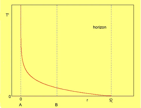
[image:5.595.234.513.493.706.2]The time function obtained we have plotted in Figure 1.
Figure 1. Time function for the dS cosmos.
It can be seen that an observer A, who starts at r=0 and travels the whole
distance from r=0 to r=R needs an infinite amount of time to get infinitely
close to the cosmic horizon. Drifting observers in the cosmos neither exceed the velocity of light nor do they even reach it.
A second observer B, released anywhere in the considered interval, reaches the horizon of A in finite time, but at a speed that is respectively lower than that of A. Since all points on a sphere are equal, any observer will call his starting point a pole. When the observer B leaves his pole, he travels through the horizon of A
with subluminal speed and he reaches his individual equator, i.e., he reaches his
horizon only asymptotically. The equator of B lies beyond the equator of A.
In an earlier paper [3] we have extended the dS cosmos to a genuine
expand-ing model by givexpand-ing up the condition R=const ., i.e., allowing an expansion of
the pseudo-hyper sphere. In this case, the observer’s motion described above is related to expansion and is responsible for the recession velocity of the galaxies. In the subluminal model we have proposed this velocity is also geometrically de-fined. We can access the same formulae as above and we get the results dis-cussed. Even in a generalized expanding model, the speed of light is the unat-tainable barrier to any motion of galaxies.
If A sends a beam of light to a galaxy B and is reflected back to A, both run-times are equal in accordance with the special theory of relativity, because B can define his position as a pole on the hypersurface. Both distances have the same length and the motion of the light source has no influence on the behavior of a light beam. This applies likewise to motions in the static model as well as to mo-tions caused by expansion in the subluminal model.
With the subluminal model one has a cosmological model at hand which sa-tisfies all requirements of special and general relativity. It is supported by Melia’s
carefully performed evaluation of observational data. Melia1 refers to the
h
R =ct model proposed by him which is flat and infinite. However in [2] and
[3] we have shown that this model is identical to our subluminal model if we
reinterpret the model of Melia using Einstein’s elevator principle. It should also
be mentioned that Chodorowski [4] [5] [6] has dealt with the question of
whether the recession velocity of the galaxies is due to an expansion of space or whether is a motion in the static space in the sense of Milne.
We have extensively dealt with the transformation of coordinate systems into
reference systems in the dS family in the papers [7][8][9]. In particular, the
pa-per of Florides [10] should be pointed out.
3. The Generalized de Sitter Model
We raise the question of whether the expansion of a cosmos can take place at a lower speed than that of free fall. We simplify the problem by studying it in the dS cosmos. We start with its static form. We define a motion by relativistically subtracting a second velocity from the velocity of free fall.
1The papers of Melia are listed in [3].
This double-velocity model will by no means describe Nature. It only serves to elaborate the mathematical methods. But it can also be stimulating to think about a genuine expanding model that expands more slowly and that predicts to have a lower recession velocity for its galaxies. This can affect the interpretation of the redshift.
To formulate the problem we use the formula apparatus of the special relativ-ity theory for relative velocities. We use the Lorentz transformations
1' 4' 1' 4'
1 1 4 4
1'' 4'' 1'' 4''
1' 1' 4' 4'
1'' 4'' 1'' 4''
1 1 4 4
, , ,
, , ,
, , ,
E E E E E E
R R R R R R
L L i v L i v L
L L i v L i v L
L L i v L i v L
α α α α
α α α α
α α α α
= = − = =
= = − = =
= = − = =
. (2.1)
Therein vR is the speed of a fictional observer driven by the dS forces. This
velocity is reduced by a second speed vE. This gives the actual recession velocity
v. In the formulae m'' tags the fictitious system, m' the physical comoving
[image:7.595.271.478.304.382.2]system, and m the static system. We illustrate this with Figure 2 below:
Figure 2. The composition of the velocities.
Furthermore, we need the formulae for the relativistic relation of the velocities
, ,
1 1 1
R E E R
R E
R E E R
v v v v v v
v v v
v v vv v v
− + −
= = =
− + − (2.2)
together with the Lorentz relations
2 2 2
1 1 v , R 1 1 vR, E 1 1 vE
α = − α = − α = − , (2.3)
(
1)
,(
1)
,(
1)
R E v vR E R E vvE E R v vR
α α α= − α =αα + α =α α − , (2.4)
(
)
,(
)
,(
)
R E R E R R E E E E R R
v v v v v v v v v
α =α α − α =αα + α =α α − . (2.5)
The analytic form of the new speed cannot be chosen arbitrarily. All quantities
which contain vE must satisfy Einstein’s field equations and the conservation
law. Furthermore, we expect that in case of reduced recession velocity radial re-pulsive forces in the comoving system still occur, but with lower strength than those in the freely falling system. Furthermore, we expect tidal forces. The latter are
easy to derive and they give first useful hints for the ansatz of the velocity vE.
In addition, we convince ourselves that the recession velocity is relativistically
defined. For the dS coordinate r applies
|1 R, |4 0
R
r
r a r r
α ∂
= = =
∂ .
Thus, one gets
{
}
{
}
| 1, 0, 0, 0 , | ' ' | , 0, 0, m
m R m m m R
r = a r =L r =
α
−i v aα
. (2.6)With 4'
dx =i Td ' one has αRdr d 'T =αv. In the dS cosmos is
1
dx =αRdr
and for the comoving system one has 1'
dx =0, dT dT′ =α. This finally results
in
1
1' d
, const .
d R
x
v v x
T = < = . (2.7)
On the other hand, one obtains from 1
dx =0, d ' dT T=α
1'
1 d
, const .
d '
x
v x
T = − = . (2.8)
The recession velocity fits the basic structure of the special theory of relativity. To calculate the new field quantities, we need the inhomogeneous transforma-tion law of the Ricci-rotatransforma-tion coefficients. Since the motransforma-tions take place in the [1, 4]-slice of the space, the [2, 3]-quantities transform homogeneously, just like vectors. Thus,
{
}
(
)
| |
' ' ' '
1 1 1
1, 0, 0, 0 , sin , cot , 0, 0
sin
,
R R
m m m m
m m
m m m m m m
a a
B r C r
r r r r r
B L B C L C
ϑ ϑ
ϑ
= = = =
= =
applies for the lateral field quantities. With (1.1) they attain the form
' '
1
, 0, 0, , , cot , 0,
R R R R
m m
a a a a
B i v C i v
r r r r r
α α α ϑ α
= − = −
. (2.9)
With this we recognize that the radial part and the timelike part of these quantities no longer appear to be flat, as it was the case for the freely falling frame of reference of the dS Model with (1.13). The formula (1.13) for free fall is
obtained only if α α= R, i.e., if vE =0. If one now demands that the comoving
volume element expands equally in all three directions one has
4' 4' ' 4'
R
a
B C U i v
r α
∗ ∗
= = = − (2.10)
and thus one has derived the timelike component of the radial quantity 'Um' of
the comoving system. Since one must obtain the same expression with the in-homogeneous transformation law of the Ricci-rotation coefficients, one can
draw conclusions about the properties of the quantity vE.
The inhomogeneous transformation law of the Ricci-rotation coefficients
' ' ' ' '
' ' ' ' ' ' ' ' ' | '
'Am ns =Am ns +'Lm ns, 'Lm ns =L Lss sn m (2.11)
can be simplified, since in the present case the Lorentz transformation is a pseudo rotation in the [1, 4]-slice of the surface. The inhomogeneous term
which we call the Lorentz term, can be expressed with hm n' '=diag 1, 0, 0,1
{
}
andcan be brought into vector form with
{
}
' ' ' ' 4' 1'
' ' ' ' ' ' ' ' ' 4'1' 1'4'
' s s' ' s, ' ' s ' , '
m n m n m n n s n
L =h L −h L L = L = L L . (2.12)
From (2.11) remains only Einstein’s elevator law[2]
{
}
' ' ' '
1 'Um Um 'Lm, Um α, 0, 0, i vα αR Rv
= + = − −
R. (2.13)
With (2.11), (2.12), and (2.1) we calculate
2 2
1' |4' 4' |1'
'L =i
α
v , 'L = −iα
v .With the help of the relation
2 2 2
dv RdvR EdvE
α =α −α
we evaluate
2 2 2 2
1' |4' |4' 4' |1' |1'
'L =i
α
R Rv −iα
E Ev , 'L = −iα
R Rv +iα
E Ev .First, we determine the first terms of these relations. In analogy to (1.14) we now have
{
}
{
}
| | '
1 1
1, 0, 0, 0 , , 0, 0,
R m R R m R
v = a v = α −i v aα
R R . (2.14)
With (2.10) and (2.13) on hand we obtain
(
)
2 2
4' |1'
2 2
|1' |1'
1 1
'
1 1
R R R R E E
R R E R E E E
U i v v i i v
i vv i v i i v
α α α αα α
αα α α α
= − ⋅ +
= − − + = − +
R R
R
.
We take the value for 'U4' from (2.10) and after some calculation we get
|1'
1
E E E
v a v
r
= . (2.15)
Furthermore, we require that the quantity vE in the comoving system is time
independent, so that we finally obtain
{
}
{
}
| ' |
1 1
1, 0, 0, 0 , , 0, 0,
E m E E E m E E
v a v v i v a v
r α α r
= = . (2.16)
Now we are also able to clearly present the Lorentz term
{
}
{
}
' ' ' ' '
1 1
'Lm Gm lm, Gm i v, 0, 0, i R , lm 0, 0, 0,1 i E Ev
r
α α α α
= − + = =
R (2.17)
and also with '
'
'
m m m m
L = −L L the inverse transformation
{
}
1{
}
1, 0, 0, 0,1 , , 0, 0,
m m m m R m E E
L G l G i l i v i v r
α α α α
= − = = −
R . (2.18)
The components G and l are assigned to the changes of vR and vE,
respec-tively.
Now we can continue with (2.13)
1'
1 1
'U = −ααR Rv +ααRv
R R.
Finally, we have with (2.5)
'
1 1
'Um E Ev , 0, 0, i vaR
r
α α
= − −
R . (2.19)
It can be seen that, in contrast to the “free falling” observer (1.12), radial forces
act on a less rapidly comoving observer
1' 1'
1 'E = −'U =αE Ev
R ,
acting repulsively. At the same time tidal forces occur.
With (2.11) we have obtained this quantity from the non-comoving system by an inhomogeneous transformation law. But since the field quantities of the freely falling system are also known, we can derive (2.19) from this system as well.
The inhomogeneous transformation law for m''→m' is
' " " ' '' ' ' ' "
' ' ' ' " '' '' ' ' ' ' " ' | '
'Am ns =Lm n sm n s "Am ns +lm ns, lm ns =L Lss sn m. (2.20)
The Lorentz term
{
2 2}
' |4', 0, 0, |1'
m E E E E
l = −iα v iα v (2.21)
leads to the simple expression
{
}
'
1 0, 0, 0,1
m E E
l i v
r α
= (2.22)
which we have already worked out on the way to (2.17). But now we can give a better justification. We write (1.12) as
{
}
" '
" m 0, 0, 0, , " m E E, 0, 0, E
i i
U = − U = −iα v α −
R R
and finally we have recovered the quantity (2.19) with
' ' '
'Um ="Um +lm. (2.23)
We have deduced all field quantities which we need for the generalized ver-sion of the dS model.
4. The Field Equations of the Generalized dS Model
The ansatz introduced in the last Section for a double-velocity model as a gene-ralization of the dS model can only be justified if the field quantities obtained sa-tisfy Einstein’s field equations. For verification, we have to process the quantities
' '
'
1
, 0, 0, , , cot , 0,
1
' , 0, 0,
R R R R
m m
R
m E E
a a a a
B i v C i v
r r r r r
a U v i v
r
α α α ϑ α
α α
= − = −
= − −
R
. (3.1)
With these quantities and the unit vectors
{
}
{
}
{
}
{
}
' 1, 0, 0, 0 , ' 0,1, 0, 0 , ' 0, 0,1, 0 , ' 0, 0, 0 1,
m m m m
m = b = c = u = (3.2)
the Riccitensor and Ricci scalar take the form
1
2 2
3 3
1 2 3
' '
' ' || ' ' ' '
' '
' || ' ' ' ' ' || ' '
' ' ' || ' ' ' ' ' || ' '
' ' ' ' ' '
|| ' ' || ' ' || '
' ' '
1
' ' '
2
s s
m n s s m n
s s
n m n m n m s s
s s
n m n m n m s s
s s s s s s
s s s s s
R U U U h
B B B b b B B B
C C C c c C C C
R U U U B B B C C
= − +
− + − +
− + − +
− = + + + + +
Cs'
. (3.3)
Therein we have used the graded derivatives [11][12]
1
2 3
'|| ' '| '
' ' '
'|| ' '| ' ' ' ' '|| ' '| ' ' ' ' ' ' '
' '
' , '
n m n m
s s s
n m n m m n s n m n m m n s m n s
U U
B B U B C C U C B C
=
= − = − − (3.4)
which allow a clear representation of the field equations. The subequations of (3.3) describe the curvatures in the radial and lateral slices of the dS space, as viewed by the comoving observers. Therefore we solve the subequations of Eins-tein’s field equations separately
(
)
2 2
3 3
' '
| ' ' 2
' '
'|| ' ' ' ' ' 2 || ' ' 2
' '
'|| ' ' ' ' ' ' ' 2 || ' ' 2
1
' ' '
1 2
,
1 3
,
s s
s s
s s
m n m n m n s s
s s
m n m n m n m n s s
U U U
B B B h B B B
C C C h b b C C C
+ = −
+ = − + = −
+ = − + + = −
R
R R
R R
. (3.5)
With this we get for the Ricci-quantities
' ' ' ' 2 2 ' ' ' ' 2 ' '
3 12 3
, ,
m n m n m n m n m n
R =g R= G = −g = −κT
R R R . (3.6)
From the last relation we get for the components of the stress-energy-momentum tensor and the equation of state
0 0
2 2
3 3
, , 0
p p
κ = − κµ = +µ =
R R . (3.7)
The values obtained are equal to those of the static dS cosmos. We note that matter transport cannot be observed in the comoving system. The cause is the
form of the equation of state. For all models with p+µ0=0 one has T1'4'=0,
as we can easily convince ourselves with the transformation ' ' ' '
m n
m n m n m n
T =L T .
5. More about the Velocities
While the velocity vR=r R is geometrically determined, we do not so far have
knowledge of the second part of the recession velocity. We only know the
change from vE which we have determined as a general feature of the model.
We have succeeded in establishing plausible field quantities which fulfill Eins-tein’s field equations and which lead to the familiar expressions for the pressure and the density of matter in the cosmos.
Now we will examine whether an analytic expression can be found which is compatible with all relations of Section 4 and provides a deeper insight into the geometric structures of the model.
We put
( )
, ' ' '
' E
r
v = R= R T
R . (4.1)
'R is a new time-dependent parameter and we notice the analogy with the
de-finition vR=r R. Thus, we can assume that vE has a similar geometrical
meaning in a fictive cosmos, which is preliminary to the dS cosmos, where vR
is well defined.
For the recession velocity of the galaxies we then have
2 '
1 '
r r v
r
− =
−
R R
R R
(4.2)
according to (2.2). For 'R R= the recession velocity is v=0. For 'R→ ∞ is
0 E
v = and v takes its maximum value, namely the dS velocity. At the cosmic
horizon, the recession velocity asymptotically reaches the velocity of light
re-gardless of the value of vE. Thus, the ranges of 'R and r are
' , 0 r
≤ ≤ ∞ ≤ ≤
R R R (4.3)
and 'R is a parameter with which one can manipulate the recession velocity
v. If this technique can be applied to a model that is closer to Nature, the
cal-culable redshift values may be better adapted to the values observed. In Figure 3,
the recession velocity is plotted in the range 0≤ ≤r R for different 'R. It can
be seen that a deviation from the linear velocity law ('R= ∞) by an appropriate
choice of 'R is possible.
Since v depends on time, as shown in (4.1) and (4.2), the generalized dS
[image:12.595.234.514.400.625.2]model allows accelerations of the drifting systems.
Figure 3. Recession velocity.
Now all we have to do is to show that the approach (4.1) meets the require-ments made in the previous sections. In particular, we have to check if
{
}
| '
1 1, 0, 0, 0
E m E E
v a v
r
= (4.4)
is well-matched with Equation (2.6) and (4.1). Following (4.1) we write
| ' | ' | '
1 1
' '
E m E m m
v v r r
= −
R R . (4.5)
Since (2.14) has already been calculated, we only need to know more about the quantity
' | '
1
' '
'
m = m
R R
R (4.6)
which we obtain by equating (4.4) with (4.5). After some calculation and re-peated use of (2.3)-(2.5) we get
'
1 1
' , 0, 0,
'
m vaR i vaR
r
α α
= − −
R
R .
We recognize that the 4th component of this quantity has already arisen as
4'
'U . Applying again the Lorentz relations leads to
{
}
{
}
' ''
' , 0, 0, , ' 0, 0, 0,1
' '
m E E E m
i i i i
iα v α
= − − = −
R R
R R R R . (4.7)
The second relation (4.7) contains the already known expression
4"
"U = −i R which results from the temporal change of the scale factor K.
Therefore the ansatz (4.1) is satisfactory and thus (4.4) can be written as
{
}
2| ' 1, 0, 0, 0 , 1 2
' '
E
E m E
a r
v = a = −
R R , (4.8)
i.e., in the same way as in (2.14). The inhomogeneous transformation law of the
Ricci-rotation coefficients can be simplified with the quantities (2.17) and (2.18), if one considers (4.1)
{
}
{
}
{
}
{
}
{
}
{
}
' '
'
1 1
0, 0, 0,1 , , 0, 0,
'
1 1
, 0, 0, , 0, 0, 0,1
'
' , 0, 0, 0, 0, 0,1
'
m R m E
m R m E
m E E E E
G i l i v i
G i v i l i
i i
U i v
α α α α
α α α α
α α α
= = −
= =
= − +
R R
R R
R R
. (4.9)
One should note the analogy of the quantities G and l.
6. Coordinate Transformations
The model described above was carried out in the tetrad calculus. A resort to a coordinate system was only necessary when basic mathematical operations had to be performed. For this, the static dS coordinate system was sufficient. Cos-mologists, however, are trying to find coordinate systems for both the comoving and the non-comoving frames of reference. We want to investigate whether coordinate systems exist for all states of motion and also transformations be-tween them. The reader who is only interested in the general structure of the model can skip this section.
Coordinate systems have been known for the static and the fictitious
ing systems since de Sitter and Lemaître. The question is, however, whether there is not only a frame of reference for the physical comoving system, but also a coordinate system.
To get closer to the problem, let us start with the static dS system
1 2 3 4
2 2
1 R, 2 , 3 sin , 4 R, R 1 R 1
e=
α
e =r e =rϑ
e =a a =α
= −r R (5.1)and the expanding one
" " " "
1 2 3 4
1" , 2" , 3" sin , 4" 1,
"
r
e e r e r e
r ϑ
=K = = = K= , (5.2)
where r is the non-comoving and r" is the comoving radial coordinate and
K the scale factor. From (5.2) it can be seen that the coordinate time and the
proper time of the drifting observers coincide (t"=T"). T" is the cosmic time
common to all drifting observers.
The coordinate transformation between the two systems has been given in
(2.9)2 and the associated Lorentz transformation in (1.11). Since the Lorentz
transformation to the physical system is known as (2.1), we first transform the static system (5.1) into the physically comoving system while maintaining the static coordinates
' '
1 4 ' 1' 4
1 1 4 4
1 1 4 4
1' 4 ' 1' 4 '
, , ,
, , , .
R R R R
R R R R
e e i v e i va e i a
e a e i va e i v e
αα α α α α
α α α α αα
= = − = =
= = − = = (5.3)
The Ricci-rotation coefficients for this system provide the values obtained in the previous Section. With the help of
' '
' '
m i m
i i i
e = Λ e (5.4)
the system can be diagonalized. For the matrix of the coordinate transformation we get
2 2 2
2 2
' '
2
2 2 2
1 , 1 1 1 1 R R R i i i i R v v i i v i v i v
α α α
α α α α α −
Λ = Λ =
−
. (5.5)
Alternatively, one can start with the freely falling dS system
' ' " ' ' " " " ", ' " '
m m m m m i
i m i i i i
e =L e e =e Λ . (5.6)
With " ' ' " 1 1 1 1 , 1 1 R R
E E E E E E
R R
i i
i i
R R
E E E E E E
R R
v
i v i v
v v
v
i v i v
α α α α
α α α α
α α α α
α α α α
α α α α
α α α α
−
Λ = Λ =
− − K K K K
2The primes on the indices of Section 2 are now to be replaced by double primes.
(5.7) one also arrives at the diagonalized system for the physical comoving observer:
' '
1 4 1' 4'
1' 4'
1' 4 '
, , R , R
R R
v
e e e e
v
α α
α α
α α α α
= = = = . (5.8)
Herewith the line element takes the form
2 2 2
2 2 2 2 2 2 2 2
2 2
d d ' d sin d d '
R R
v
s
α
r rϑ
rϑ ϕ
α
tα
α
= + + − . (5.9)
The two observer transformations (5.5) and (5.7) are related to the holonomic Lemaître transformation (1.9) by
" " ' " "
' , |
i i i i i
i i i i x i
Λ = Λ Λ Λ = .
It can be seen that there is no cosmic universal time for the comoving physical observer system. Rather, one has for the proper time of the observers
d ' d '
R
T α t
α
= (5.10)
in accordance with the general theory of relativity.
However, the Ricci-rotation coefficients cannot be derived from the 4-bein system (5.8), as we have learned in the previous sections. The reason is the an-holonomicity of the two coordinate transformations (5.5) and (5.7). One easily convinces oneself that
[ ]|' 0 ' '|, [" | "' ] 0 "' '| "
j j j j j j
i i i i
i k x i k x
Λ ≠ ⇒ Λ ≠ Λ ≠ ⇒ Λ ≠ . (5.11)
Thus, there exists no associated global coordinate mesh for the comoving ob-server system, but only anholonomic coordinates. These are mathematical
arti-facts described in detail by Schouten [13].
If one proceeds in the usual way and elaborates with (5.8) the expression
' '
'
' ' ' ' ' ' ' '
' ' ' ' ' ' ' ' '
[ ' | '] [ ' | '] [ ' | ']
t t
s
s j s r j s r j
m n j n t j m t j
n m r m r n
A =e e +g g e e −g g e e
and if one then complements the object of anholonomity
[ ] '
' '
' '
' ' ' ' | '
' ' s
i k
s j j
m n j j k i
m n
e e e
Λ = Λ Λ (5.12)
one finally gains the Ricci-rotation coefficients
' ' ' ' '
' ' ' ' ' ' ' ' ' '
' s s s s s
m n m n m n m n n m
A =A + Λ + Λ + Λ (5.13)
with the values known of Section 3.
It is clear that the search for coordinate systems which accompany the families of observers is not necessary and often not practical.
7. Conclusions
We have proposed a model which we do not assume to be realized by Nature.
However, it includes useful mathematical techniques which can be transferred to more sophisticated models. In particular, it is possible to reduce the recession
velocity of the galaxies compared to those of the “free fall” and thus to manipu-late the calcumanipu-lated values for the redshift. This could allow a better adjustment to the observed values.
In the next step, by dropping the relation R=const ., we want to examine a
genuine expanding model with these methods. We hope to publish this else-where.
References
[1] Lemaître, G. (1933) Annales de la Société scientifique de Bruxelles, A53, 51-85. [2] Burghardt, R. (2016) Journal of Modern Physics, 7, 2347-2356.
https://doi.org/10.4236/jmp.2016.716203
[3] Burghardt, R. (2017) Journal of Modern Physics, 8, 583-601.
https://doi.org/10.4236/jmp.2017.84039
[4] Chodorowski, M.J. (2016) A Direct Consequence of the Expansion of Space? https://arxiv.org/pdf/astro-ph/0610590.pdf
[5] Chodorowski, M.J. (2005) Cosmology under Milne’s Shadow. https://arxiv.org/pdf/astro-ph/0503690.pdf
[6] Chodorowski, M.J. (2008) Eppur si muove. https://arxiv.org/pdf/0812.3972.pdf [7] Burghardt, R. (2016) Austrian Reports on Gravitation.
http://members.wavenet.at/arg/Wpdf/WTrans1.pdf [8] Burghardt, R. (2016) Austrian Reports on Gravitation.
http://members.wavenet.at/arg/Wpdf/WTrans2.pdf [9] Burghardt, R. (2016) Austrian Reports on Gravitation.
http://members.wavenet.at/arg/Wpdf/WTrans3.pdf
[10] Florides, P.S. (1980) GRG, 12, 563-574. https://doi.org/10.1007/BF00756530 [11] Burghardt, R. (2016) Spacetime Curvature. 1-597.
http://members.wavenet.at/arg/EMono.htm [12] Burghardt, R. (2016) Raumkrümmung. 1-623.
http://members.wavenet.at/arg/Mono.htm
[13] Schouten, J.A. (1954) Ricci-Calculus. Springer, Berlin Heidelberg. https://doi.org/10.1007/978-3-662-12927-2