University of Warwick institutional repository:
http://go.warwick.ac.uk/wrap
A Thesis Submitted for the Degree of PhD at the University of Warwick
http://go.warwick.ac.uk/wrap/72853
This thesis is made available online and is protected by original copyright.
Please scroll down to view the document itself.
M A
E
G
NS I
T A T MOLEM
U N
IV
ER
SITAS WARWICEN
SIS
The Temporal and Spatial Analysis of
Single Cell Gene Expression
by
Kirsty Hey
Thesis
Submitted to the University of Warwick
for the degree of
Doctor of Philosophy
Department of Statistics, University of Warwick
CONTENTS
List of Figures vii
List of Tables xii
Acknowledgements xiii
Declarations xiv
Abstract xv
Chapter 1 Introduction 1
1.1 Biological Background . . . 2
1.1.1 Gene Expression . . . 2
1.1.2 Experimental Techniques . . . 3
1.2 Motivating Data . . . 5
1.2.1 Temporal Dynamics . . . 6
1.2.2 Spatial Organisation . . . 8
1.2.3 Spatial Coordination . . . 9
1.3 Thesis Outline . . . 10
I Temporal Analysis of Gene Transcription 12 Chapter 2 Stochastic Reaction Networks 13 2.1 Introduction . . . 13
2.2 Exact Inference . . . 17
2.3.1 Macroscopic Limit . . . 20
2.3.2 Limiting Diffusion Processes . . . 21
2.3.3 Birth Death Approximation . . . 26
2.3.4 Other Approximations . . . 30
2.4 Comparative Study . . . 31
Chapter 3 Inference for State Space Models of Stochastic Gene Tran-scription 34 3.1 State Space Representation . . . 34
3.2 Filtering, Smoothing and Backward Sampling . . . 37
3.2.1 Filtering . . . 37
3.2.2 Smoothing and Backward Sampling . . . 38
3.3 Towards an Inference Framework . . . 39
3.4 The Likelihood . . . 40
3.4.1 Exact Likelihood . . . 40
3.4.2 LNA Likelihood . . . 40
3.4.3 BDA Likelihood . . . 43
3.4.4 Likelihood Comparison . . . 51
3.5 Parameter Inference . . . 57
3.5.1 Random Walk Metropolis Hastings . . . 57
3.5.2 Reversible Jump MCMC scheme . . . 58
3.5.3 Hierarchical Model . . . 59
3.6 Prior Specification . . . 63
3.7 Inferring the Latent States . . . 65
3.7.1 Particle Gibbs . . . 65
3.7.2 Particle Marginal Metropolis Hastings . . . 67
3.8 Algorithm Specification . . . 67
3.9 Simulation Study . . . 69
3.9.1 Study Design . . . 69
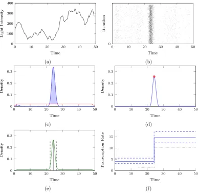
3.9.2 Illustrative Example . . . 70
3.9.3 Results . . . 84
Chapter 4 Application to Single Cell Imaging Data 91
4.1 Pre-processing . . . 92
4.2 Preliminary Analysis . . . 96
4.3 Stochastic Switch Tool Specification . . . 97
4.4 Illustrative Example . . . 98
4.5 Posterior Analysis . . . 100
4.5.1 Parametric Transcriptional Process . . . 108
4.6 Discussion . . . 116
II Spatial Organisation of Lactotroph Cells 122 Chapter 5 Spatial Point Processes 123 5.1 Introduction . . . 123
5.2 Basic Principles . . . 124
5.3 Exploratory Analyses of Stationary Point Processes . . . 127
5.4 Cox Processes . . . 130
5.5 Gibbs Processes . . . 131
5.5.1 Hybrid Gibbs Processes . . . 137
5.5.2 Model Fitting . . . 138
5.6 Literature Examples . . . 143
Chapter 6 Application to Single Cell Imaging Data 145 6.1 Introduction . . . 145
6.2 Exploratory Analyses . . . 147
6.2.1 Intensity Analysis . . . 148
6.2.2 Network Analysis . . . 149
6.2.3 Summary Statistics . . . 152
6.3 Point Process Modelling . . . 155
6.3.1 Model Fitting . . . 155
6.3.2 Results . . . 159
III Spatio-Temporal Coupling of Gene Transcription 168
Chapter 7 Spatial Transcriptional Dynamics 169
7.1 Introduction . . . 169
7.2 Biological Coupling . . . 170
7.3 Spatial Score Functions . . . 171
7.4 Spatial Likelihood . . . 180
7.4.1 Spatial Transition Times . . . 182
7.4.2 Spatial Transcriptional Levels . . . 183
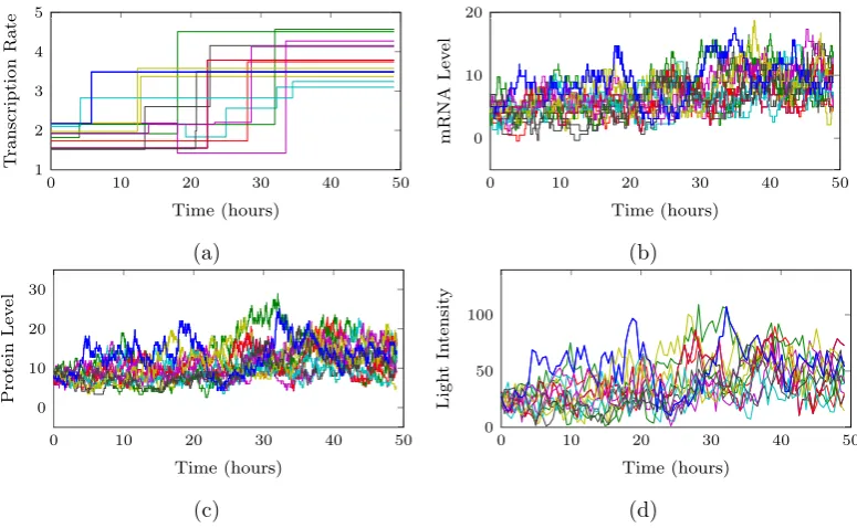
7.5 Simulation Model . . . 184
7.5.1 Hub Behaviour . . . 185
7.5.2 Correlation Behaviour . . . 185
7.6 Towards an Inferential Framework . . . 189
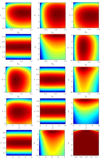
7.6.1 Parameter Identifiability . . . 192
7.6.2 Model Identifiability . . . 193
7.7 Discussion . . . 196
IV Summary 198 Chapter 8 Future Work, Extensions and Conclusions 199 8.1 Future Work and Extensions . . . 199
8.2 Conclusions . . . 201
V Appendices and Bibliography 202 Appendix A Supplementary Review Material 203 A.1 Exact Inference Approaches . . . 203
A.2 Alternative Approximations . . . 207
Appendix B Technical Appendices 211 B.1 Transition Densities for SRNs . . . 211
B.2 Reparameterisation of the LNA . . . 214
Appendix C Figures 217
References 227
LIST OF FIGURES
1.1 Illustration of gene expression. . . 3
1.2 Diagrammatic representation of the measurement process through reporter genes. . . 4
1.3 Example data of single cell Prolactin gene expression measured through a GFP reporter. . . 6
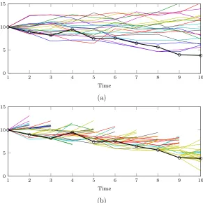
2.1 Simulation envelopes for M∗ in the BDA under three different ap-proximations. . . 27
2.2 Simulation envelopes for protein populations under three different approximations ofM∗ under the BDA. . . 28
2.3 Empirical transition densities for protein populations under three dif-ferent approximations ofM∗ under the BDA. . . 28
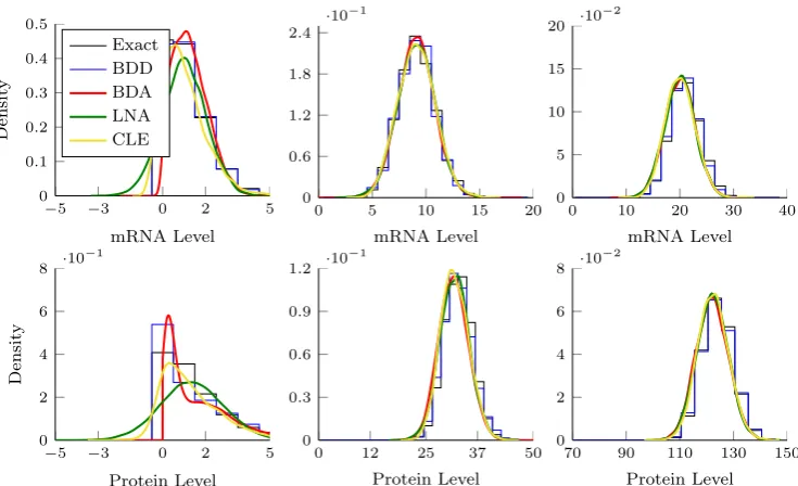
2.4 Empirical transition densities for the exact SRN, the BDD, BDA, LNA and CLE. . . 32
2.5 Simulation envelopes for the exact SRN, the truncated normal BDA, the LNA and the CLE. . . 33
3.1 A pictorial representation of a general hidden Markov model. . . 35
3.2 Illustration of weight degeneracy and particle degeneracy. . . 48
3.3 Bivariate likelihood transects under the exact joint likelihood. . . 52
3.4 Bivariate likelihood transects under the LNA joint likelihood. . . 53
3.5 Bivariate likelihood transects under the BDA joint likelihood. . . 54
3.6 Bivariate likelihood transects under the restarting LNA data likelihood. 55 3.7 Bivariate likelihood transects under the non-restarting LNA data like-lihood. . . 56
3.10 Thinned Markov chains under the BDA. . . 72
3.11 Posterior densities under the LNA. . . 73
3.12 Posterior densities under the BDA. . . 74
3.13 Illustrative example of fitting a marginal parametric switch model to
the posterior samples under the LNA. . . 76
3.14 Illustrative example of fitting a marginal parametric switch model to
the posterior samples under the LNA. . . 77
3.15 Posterior density of the number of switches sampled under the LNA. 78
3.16 All possible sub-models of a three switch marginal model. . . 79
3.17 All possible sub-models for transcription for two example cells
esti-mated via the reversible jump procedure. . . 81
3.18 Diagnostic plots of the posterior switch model under the LNA. . . . 83
3.19 Diagnostic plots of the posterior switch model under the BDA. . . . 84
3.20 Mean square error under each methodology for the different simula-tion scenarios. . . 86
3.21 The width of the 50% credible intervals under each methodology for the different simulation scenarios. . . 87
3.22 WAIC comparison for the LNA and BDA methodologies. . . 89
4.1 Light intensity measurements from two separate channels and the
resulting combined measurements. . . 94
4.2 Illustration of combining two channels of light intensity measurements. 95
4.3 The residuals of the linear fit between the two channel measurements
as shown in Figure 4.2. . . 95
4.4 Time series data of eight different datasets. . . 96
4.5 Autocorrelation function of the time series shown in Figure 4.4. . . . 97
4.6 Subset of data, to illustrate the LNA and BDA methodologies. . . . 98
4.7 Single cell example of the transcriptional back-calculation. . . 99
4.8 Marginal posterior transcriptional profiles. . . 101
4.9 The back-calculated marginal posterior of the log translation
trans-formed transcriptional profiles. . . 102
4.10 A representative sample of posterior transcriptional profiles. . . 103
4.11 Histograms of the number of switches in the posterior transcriptional profile. . . 105
4.13 Combined histograms of the number of switches in the posterior
tran-scriptional profile. . . 107
4.14 Proportion of cells with more than two transcriptional switches. . . . 107
4.15 Density estimate of the inter-switch waiting times. . . 108
4.16 Illustration of the binary switch model. . . 109
4.17 Posterior transcriptional waiting times between successive switches. . 117
4.18 Illustration of the multi-state switch model. . . 118
4.19 Fitting a model to the observed waiting times between consecutive switches. . . 119
4.20 Boxplots showing how the type of next switch depends on the current transcriptional rate. . . 119
4.21 Density plots of how the current transcriptional rate changes with the type of next switch. . . 120
4.22 Linear regression fits between consecutive transcriptional rates. . . . 120
4.23 The relationship between the time spent in any transcriptional state and the level of transcription. . . 121
5.1 Realisations of three different spatial point processes. . . 127
5.2 Realisation of a hardcore process. . . 133
5.3 Illustration of a two component multiscale process. . . 135
6.1 The spatial location of individual cells within datasets A1-A3, P1-P2 and E1. . . 147
6.2 Spatial intensity analysis of the location of individual cells within datasets A1-A3, P1-P2 and E1. . . 148
6.3 Example of the Euclidean network for dataset P1. . . 150
6.4 Examples of the Euclidean network for dataset A3. . . 150
6.5 Geodesic network examples for datasets P1 and A3. . . 151
6.6 Geodesic networks for dataset A1. . . 151
6.7 Observed L-,J- and pair correlation functions for each dataset com-pared to a homogeneous Poisson process. . . 153
6.8 Observed L-,J- and pair correlation functions for each dataset com-pared to an inhomogeneous Poisson process. . . 154
6.10 Summary statistics of the fitted hardcore Strauss model to dataset A2.156
6.11 Profile pseudo-likelihood for the range of interaction in a hybrid
hard-core Strauss Area-Interaction model of dataset A2. . . 157
6.12 Summary statistics of the fitted hybrid hardcore Strauss and Area-Interaction model to dataset A2. . . 158
6.13 Residuals of a fitted point process to dataset A2. . . 159
7.1 The relationship between the Pearson correlation coefficient of any two time series and the pairwise Euclidean distance. . . 170
7.2 Illustration of the different spatial Score functions. . . 172
7.3 Relationship between each Score function for dataset A1. . . 173
7.4 The relationship between Score 2 and Euclidean distance for datasets A1-A4. . . 175
7.5 The relationship between Score 1 and Euclidean distance. . . 175
7.6 The relationship between Score 1 and Euclidean distance for datasets A1-A4. . . 175
7.7 The spatial distribution of Feature 1. . . 177
7.8 The spatial distribution of Feature 2. . . 177
7.9 The spatial distribution of Feature 3. . . 178
7.10 The spatial distribution of Feature 4. . . 178
7.11 Illustration of how the parameter p varies over distance under three different definitions given in the main text. . . 183
7.12 Simulating spatial hub behaviour. . . 186
7.13 Simulating spatial correlation behaviour through different spatial de-pendencies. . . 187
7.14 Simulating spatial correlation behaviour through different transcrip-tional models. . . 188
7.15 Simulating spatial correlation behaviour as the threshold distance varies. . . 188
7.16 Simulating spatial correlation behaviour as the threshold time varies. 188 7.17 Profile likelihood transects of spatial transcriptional model 1. . . 190
7.18 Bivariate likelihood surface of spatial transcriptional model 1. . . 191
7.19 Profile likelihood transects as the number of cells varies. . . 192
7.21 Likelihood comparison of different transcriptional models. . . 195
B.1 Example variograms. . . 216
C.1 Boxplots of each individual time series for all datasets. . . 218
C.2 Recursive residuals of the posterior model for a single A1 time series. 219 C.3 Posterior densities estimated via the LNA on the subset of dataset P1.220 C.4 Posterior densities estimated via the BDA on the subset of dataset P1.221 C.5 Posterior densities estimated via the LNA on the subset of dataset A1.222 C.6 Posterior densities estimated via the BDA on the subset of dataset A1.223 C.7 Box-Cox transform of the correlation-distance relationship. . . 224
C.8 Variograms for spatial feature 1. . . 224
C.9 Variograms for spatial feature 2. . . 225
C.10 Variograms for spatial feature 3. . . 225
LIST OF TABLES
3.1 Model comparison of the different transcriptional profiles sampled in
the reversible jump MCMC. . . 82
4.1 Parameter estimates of fitting a parametric model to the waiting time
distributions of the marginal transcriptional process. . . 112
4.2 Parameter estimates of fitting a parametric model to the waiting time
distributions of the weighted conditional transcriptional process. . . 112
4.3 Parameter estimates of the linear regression model fitted to the weighted
conditional transcriptional process. . . 114
6.1 Threshold ranges for the existence of Euclidean networks. . . 151
6.2 Estimated parameter values of the fitted hybrid Gibbs models for
ACKNOWLEDGEMENTS
First of all I would like to thank my supervisor Dr B¨arbel Finkenst¨adt for her
guidance and support throughout the past years. Her advice and encouragement
have helped shape both this research and me as a researcher. In addition, I would like
to thank Prof. David Rand and the research group as a whole (both current and past
members) for many stimulating discussions and general solidarity at Friday morning
group meetings. The collaborative nature of this project has been truly enjoyable
due to the general enthusiasm to share both data and ideas. Acknowledgement
should be given to the labs of both Mike White and Julian Davis. In particular, I’d
like to thank Karen Featherstone for her patience with my many biology questions
and also for letting me see first hand the experimental procedures.
The Department of Statistics has provided me with many opportunities to broaden
my knowledge and expertise through funding to attend numerous conferences and
workshops. Additionally, the Engineering and Physical Sciences Research Council
has provided me with financial support (EPSRC grant number ASTAA1112.KXH)
throughout my studies.
To my friends, old and new, whether it’s Axel for patiently describing SMC, Kasia
for introducing me to green tea, Silvia for shared commiserations of non-converging
MCMC or Lorna and Cata for the shared enjoyment of apple cake. Along with
many others you have made my time at Warwick all the more enjoyable.
A special thanks to my family, for always being there. Words can’t express the
DECLARATIONS
This thesis is submitted to the University of Warwick in support of my application
for the degree of Doctor of Philosophy. It has been composed by myself and has not
been submitted in any previous application for any degree.
All experimental data discussed in this thesis have been kindly provided by the
labs of Mike White and Julian Davis at the University of Manchester. In
partic-ular, acknowledgement should be given to Karen Featherstone who performed the
experimental procedures.
In addition, Chapter 7 is collaborative work with Hiroshi Momiji whose contribution
greatly aided both the methodology and analysis.
Parts of this thesis have been published by the author in the following publication:
K Hey, H Momiji, K Featherstone, J Davis, M White, D Rand and B Finkenst¨adt
(2015). Inference for a Transcriptional Stochastic Switch Model from
ABSTRACT
It is the aim of this thesis to provide a rigorous and comprehensive analysis of single
cell gene expression data. Specifically, the focus is on expression of the human
Pro-lactin gene, which can be measured in intact tissue samples via a reporter process.
To do this, we develop a robust statistical procedure, the stochastic switch model,
to model the transcriptional regulation within single cells that properly accounts for
both intrinsic and extrinsic variability whilst also incorporating a realistic
measure-ment process. The stochastic switch model provides a highly flexible framework for
coupling the regulatory system without the need for detailed prior knowledge of the
underlying regulatory mechanisms. In this thesis, this methodology is applied to
numerous datasets to find different regulatory behaviour evident in different
biolog-ical conditions. Moreover, since the data provided has in addition a representative
spatial resolution, we investigate how the spatial organisation of the expressing cells
changes in these different biological conditions. This is achieved via spatial point
processes and makes use of the recently developed hybrid Gibbs processes. The
thesis ends by revisiting the transcriptional regulation within single cells and how
analysing these processes in space reveals evidence of cell signalling. From this
evidence, various semi-mechanistic models are derived with attention focused on
model identifiability. Consequently, this thesis provides both methods and analysis
for the temporal, the spatial and the spatio-temporal data regarding single cell gene
CHAPTER
1
INTRODUCTION
So perhaps the best thing to do is to
stop writing introductions and get on with the book.
A.A. Milne, Winnie-the-Pooh
During the last few decades there have been huge advances in experimental biology and the techniques employed that have yielded many interesting and important
in-sights into the underlying biological processes. With increasing frequency, many of
these processes have been shown to have stochastic variation at the molecular level. Moreover, as experiments become increasingly complex, relating the biology to the
measured outcomes becomes challenging. It has therefore become clear that robust
and rigorous statistical analysis is key to extracting information from such experi-ments. The objective of this research is to provide robust statistical methodology
for the analysis of gene expression dynamics where observations consist of single cell
measurements of reporter protein levels. Section 1.1 provides a basic introduction to the fundamentals of gene expression and the particular experimental techniques
to which we focus our attention. Motivating data is presented in Section 1.2 and
1.1
Biological Background
1.1.1 Gene Expression
Information encoded within individual genes is transferred through the process of
gene expression. This process results in the synthesis of some gene product, which most commonly is a specific protein that is required for some role within the body.
Examples include the production of hormones that in turn regulate physiology and
behaviour. Consequently, the regulation of gene expression within single cells en-ables individual cells to control and respond to the molecular environment. For
example, the expression of the Prolactin hormone will be highly up-regulated in response to lactation in order to produce increasing amounts of milk.
Gene expression typically consists of three main processes:
Gene activation/regulation. For a gene to be expressed it first has to be
ac-tivated. This activation occurs through a series of reactions including the
binding and/or unbinding of transcription factors to the gene promoter region of the DNA.
Transcription. Once a gene has been activated, it can be transcribed to result in
the production of mRNA molecules.
Translation. The mRNA molecules will then move out of the cell nucleus and into
the cytoplasm to either be degraded or translated into proteins. Proteins are the final product of gene expression and will move on to play some role either
within the same cell or somewhere else within the body.
The above processes are depicted in Figure 1.1, which provides a coarse level
rep-resentation. There are many other molecular processes involved in gene expression, including protein folding and unfolding, which we do not consider in our applications
due to the limited resolution of the data available.
In single cells, gene expression is made up of fundamentally stochastic processes (Raj
and Van Oudenaarden, 2008) due to bothintrinsicandextrinsicvariation. Intrinsic
variability is the variation observed between the molecular processes of identical gene
copies, which arise from random microscopic events determining these processes. For instance the reactions involved within these processes will occur randomly
accord-ing to the law of mass action and thus the event of a successful reaction will be a
(a) (b)
Figure 1.1: Illustration of gene expression where in a) the gene is activated through the binding of certain molecules to allow mRNA molecules to be created through transcription. Following this, shown in b), the mRNA molecules then move out of the nucleus and into the cytoplasm to either degrade or be translated into proteins.
extrinsic variability is the intercellular variability of gene expression caused by fluc-tuations in molecular activity due to both interacting processes and randomness in
molecular machinery (Elowitz et al., 2002). This can be interpreted mathematically
by considering fluctuations in the reaction rate constants across differing cells. Con-sequently, one must incorporate both these sources of stochasticity when analysing
gene expression within single cells.
Analysing gene expression data has attracted much attention (see for example, Kærn et al. (2005); Raj and Van Oudenaarden (2008); Spiller et al. (2010); Zechner et al.
(2014)) with many interesting features having been elicited. The main feature we
investigate in this thesis is the pulsatile behaviour of expression that has been found for many different genes (Suter et al., 2011; Harper et al., 2011). In particular, this
pulsatility has been shown to be highly variable between individual cells. Recent papers (Blake et al., 2006; Paszek et al., 2010; Harper et al., 2010, 2011) hypothesise
this varying pulsatile behaviour to be necessary for robust tissue level response to
a range of physiological conditions and we will investigate this further for a single gene application.
1.1.2 Experimental Techniques
There are many different techniques used to collect data on gene regulation and
expression. Examples include microarray experiments where the concentration of mRNA molecules is measured from aggregated data or qPCR (quantitative
poly-merase chain reaction) experiments, which measure something proportional to the
DNA
mRNA
reporter mRNA
Protein
reporter Protein
Light Intensity
∅
∅
∅
∅
translation
degradation degradation
translation
degradation degradation
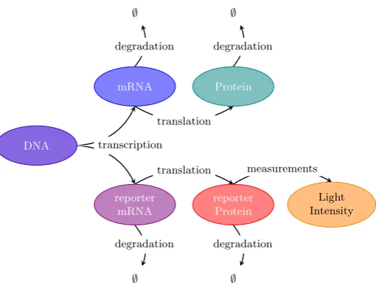
[image:21.595.185.459.108.314.2]measurements transcription
Figure 1.2: A diagrammatic representation of how the measurement process through reporter genes relates to the underlying process of native gene expression. Specifically, both native and reporter mRNA are transcribed in parallel, after which the two processes become independent with the reporter mRNA being translated into reporter protein independently of the translation of native mRNA. The reporter protein can then be measured through light microscopy techniques.
aggregated over many cells and represent an average behaviour. Here, however, we
are particularly interested in quantifying the dynamics within individual cells.
Mea-surements on individual cells can be obtained through live cell imaging techniques and has proven successful for studying the stochastic temporal expression dynamics
of reporter genes (Stephens and Allan, 2003; Spiller et al., 2010). A reporter gene is a gene that is inserted into cell DNA and engineered to be controlled by the same
promoter as the gene of interest. Examples of reporter genes are the genes coding
for fluorescent and luminescent proteins, which can be measured indirectly through light microscopy. Figure 1.2 gives a diagrammatic representation of how expression
of the reporter gene relates to native gene expression. Specifically, since the reporter
is under the control of the native gene promoter, both reporter and native mRNA will be transcribed in parallel. The reporter mRNA will then be translated into
reporter protein independently of the native mRNA. Levels of these reporter
pro-teins can then be measured indirectly through light microscopy. For instance for a green fluorescent protein, under a laser, levels of fluorescence can be measured and
will be proportional (with error) to the number of reporter protein molecules.
2002; Nelson et al., 2004; Paulsson, 2005),
DNA−−−→β(t) mRNA, mRNA−−−→ ∅δm , (1.1)
mRNA−−−→α mRNA + Protein, Protein−−−→ ∅δp , (1.2)
where the superscript for each reaction denotes the corresponding reaction rate. The
rate of transcription,β(t), will be time varying as it depends on the activation state
of the underlying gene and will therefore represent the regulation of the underlying
gene promoter. Moreover, these transcriptional dynamics of the reporter will relate
to the transcriptional dynamics of the native gene (Finkenst¨adt et al., 2008; Harper
et al., 2011) due to the coupling depicted in Figure 1.2. Consequently, it is these
transcriptional dynamics that relate the observed reporter gene expression dynamics
to the regulation of the native gene of interest, also termed the target gene.
1.2
Motivating Data
Representative data following the above reporter construction are shown in Figure
1.3. The target gene for these data is the Prolactin (PRL) gene whose regulation
is of particular interest, due to its important roles in mammalian reproduction and also its frequent over-production by pituitary adenomas (Harper et al., 2010). In
order to obtain measurements, a line of transgenic rats was created. Specifically, the
rat genome was modified so that the native DNA contained the human Prolactin promoter that in turn controlled the expression of a destabilised green fluorescent
reporter protein. Since rats naturally produce the regulatory transcription factors that bind to the human Prolactin promoter, this rat model allows one to study the
regulation of the human Prolactin gene within mammalian tissue, specifically rat
pituitary tissue. A number of different samples have been collected from different physiological conditions. Namely, pituitary tissue has been taken from animals in
different stages of development ranging from adulthood to post-natal day 1.5 and
embryonic day 18.5. Further details of the reporter construct used and associated experimental framework can be found in Semprini et al. (2009); Harper et al. (2010)
and Featherstone et al. (2011).
As an example, two representative datasets are shown in Figure 1.3 where the top row corresponds to a pituitary tissue sample taken from an adult male rat and the
bottom row corresponding to a pituitary tissue sample of a post-natal day 1.5 rat.
(a)
0 20 40
1 2
·104
Time (hours) Ligh t In tensit y (b)
0 50 100 150
−0.5
0 0.5 1 Lag Auto cor rel a ti o n (c)
0 50 100
−0.5
0 0.5 1 ● ●● ● ● ● ● ● ● ● ● ● ● ● ● ●● ● ● ● ● ● ● ● ● ● ● ● ● ● ● ● ● ● ● ● ● ● ● ● ● ● ● ● ● ● ● ● ● ● ● ● ● ● ● ● ● ● ●●● ● ● ● ● ● ● ● ● ● ● ● ● ● ● ● ● ● ● ● ● ● ● ● ● ● ● ● ● ● ● ● ● ● ● ●● ● ● ● ● ● ● ● ● ● ● ● ● ● ● ● ● ● ● ● ● ● ● ● ● ● ● ● ●● ● ● ● ● ● ● ● ● ● ● ● ● ● ● ●● ● ● ● ● ● ● ● ● ● ● ● ● ●● ● ● ● ● ● ● ● ● ● ● ● ● ● ● ● ● ● ● ● ● ● ● ● ● ● ● ● ● ● ● ● ● ● ● ● ● ● ● ● ● ●● ● ● ● ● ● ● ● ● ● ● ● ● ● ●● ● ●● ● ● ● ● ● ● ●● ● ● ● ● ● ● ● ● ● ● ● ● ● ● ● ● ● ● ● ● ● ● ● ● ● ● ● ● ● ● ● ● ● ● ● ● ● ● ● ● ●● ● ● ● ● ● ● ● ● ● ● ● ● ● ● ● ● ● ● ● ● ● ● ● ● ● ● ● ● ● ● ● ● ● ● ● ● ● ● ● ● ● ● ● ● ● ● ● ● ● ● ● ● ● ● ● ● ● ● ● ● ● ● ● ● ● ● ● ● ● ● ● ● ● ● ● ● ● ● ● ● ● ● ● ● ● ● ●● ● ● ● ● ● ● ● ● ● ● ● ● ● ● ● ● ● ● ● ● ● ● ● ●● ● ● ● ● ● ● ● ●● ● ● ● ● ● ● ● ● ● ● ● ● ● ● ● ● ● ● ● ● ● ● ● ● ●● ● ● ● ● ● ● ● ● ● ● ● ● ● ● ● ● ● ● ● ● ● ● ● ● ● ● ● ● ● ● ●● ●● ● ● ● ● ● ● ● ● ● ● ● ● ● ● ● ● ● ● ● ● ● ● ● ● ● ● ● ● ● ● ● ● ● ● ● ● ● ● ● ● ● ● ● ● ● ● ● ● ●● ● ● ● ● ● ● ● ● ● ● ● ● ● ● ● ● ● ● ● ● ● ● ● ● ● ● ● ●● ● ● ● ● ● ●● ● ● ● ● ● ● ● ● ● ● ● ● ● ● ● ● ● ● ● ● ● ● ●● ● ● ● ● ● ● ● ● ● ● ● ● ● ● ● ● ● ● ● ● ● ● ● ● ● ● ● ● ● ● ● ● ● ● ● ● ● ● ● ● ● ● ● ● ● ● ● ● ● ● ● ● ● ● ● ● ● ● ● ● ● ● ● ● ● ● ● ● ● ● ● ●●● ● ● ● ● ● ● ● ● ● ● ● ● ● ● ● ● ● ● ● ● ● ● ● ● ● ● ● ● ● ● ● ● ● ● ● ● ● ● ● ● ● ● ● ● ● ● ● ● ● ● ● ● ● ● ● ● ● ● ● ● ● ● ● ● ● ● ● ● ● ● ●●●● ● ● ● ● ● ● ● ● ●●● ● ● ● ● ● ● ● ● ● ● ● ● ●● ● ● ● ● ● ● ● ● ● ● ● ●● ● ● ● ● ● ● ● ● ● ● ● ● ● ● ● ● ● ● ● ● ● ● ● ● ● ● ● ● ● ● ● ● ● ● ● ● ● ● ● ● ● ●● ● ● ● ● ● ● ● ●●● ● ● ● ● ● ●● ● ● ● ● ● ● ● ● ● ● ● ● ● ● ● ● ● ● ● ● ●● ● ● ● ● ● ● ● ● ● ● ● ● ● ● ● ● ● ● ● ● ● ● ● ● ● ● ● ● ● ● ● ● ● ● ● ● ● ● ● ●● ● ● ● ● ● ● ● ● ● ● ● ● ● ● ●● ● ● ● ● ● ● ● ● ● ● ● ● ● ● ● ● ● ● ● ● ● ● ● ● ●● ● ● ● ● ● ● ● ● ● ● ● ● ● ● ● ● ● ● ● ● ● ● ● ● ● ● ● ● ● ● ● ● ● ● ● ● ● ● ● ● ● ● ● ● ● ● ● ● ● ● ● ●● ● ● ● ● ● ● ● ● ● ● ● ● ● ● ● ● ● ● ● ● ● ● ● ● ● ● ● ● ● ● ● ● ● ●●● ● ● ● ● ● ● ● ● ● ● ● ● ● ● ● ● ● ● ● ● ● ● ● ● ● ● ● ● ● ● ● ● ● ● ● ● ● ● ● ● ● ●● ● ● ● ● ● ● ● ● ● ● ● ● ● ● ● ● ● ● ● ● ● ● ● ● ● ● ● ● ● ● ● ● ● ● ● ● ● ● ● ● ● ● ● ● ●● ● ● ● ● ● ● ● ● ● ● ● ● ● ● ● ● ● ● ● ●● ● ● ● ● ● ● ● ● ● ● ● ● ● ● ● ● ● ● ● ● ● ● ● ● ● ● ● ● ● ● ● ● ● ● ● ● ● ● ● ● ● ● ● ● ● ● ● ● ● ● ● ● ● ● ● ● ● ● ● ● ● ● ● ● ● ● ● ● ● ● ● ● ● ● ● ● ● ● ● ● ● ● ●● ● ● ● ● ● ● ●● ● ● ● ● ● ● ● ● ● ● ● ● ● ● ● ● ● ● ● ● ● ● ● ● ● ● ● ● ● ●● ● ● ● ● ● ● ● ● ● ● ● ● ● ● ● ● ● ● ● ● ● ● ● ● ● ● ● ● ● ● ● ● ● ● ● ● ● ● ● ● ● ● ● ● ● ● ● ● ● ● ● ● ● ● ● ● ● ● ● ● ● ● ● ● ● ● ● ● ● ● ● ● ● ● ● ● ● ● ● ●● ● ● ● ● ● ● ● ● ● ● ● ● ● ● ● ● ● ● ●● ● ● ● ● ● ● ● ● ● ● ● ● ● ● ● ● ● ● ● ● ● ● ● ● ● ● ● ● ● ● ● ● ● ● ● ● ● ● ● ● ● ● ● ● ● ● ● ● ● ● ●● ● ● ● ● ● ● ● ● ● ● ● ● ● ● ● ● ● ● ● ●● ● ● ● ● ● ● ● ● ● ● ● ● ● ● ● ● ● ● ● ● ● ● ● ● ● ● ● ● ● ● ●● ● ● ● ● ● ● ● ● ● ● ● ● ● ● ● ● ● ● ● ● ● ● ● ● ● ● ● ● ● ● ● ● ● ● ● ● ● ● ● ● ● ● ● ● ● ● ● ● ● ● ● ● ● ● ● ● ● ● ● ● ●● ● ● ● ●● ● ● ● ● ● ● ● ● ● ● ● ● ● ● ● ● ● ● ● ● ● ● ● ● ● ● ● ● ● ● ●● ● ● ● ● ● ● ● ● ● ● ●● ●● ● ● ●● ● ● ● ● ● ● ● ● ● ● ● ● ● ● ● ● ● ● ● ● ● ● ● ●● ● ● ● ● ● ● ● ● ● ● ●● ● ● ● ● ● ●● ● ● ●● ● ● ● ● ● ● ● ● ● ● ● ● ● ● ● ● ● ● ● ●● ● ● ● ● ● ● ●● ● ● ● ● ● ● ● ● ● ● ● ● ● ● ● ● ● ● ● ● ● ● ● ● ● ● ●● ● ● ● ● ● ● ●● ● ● ● ● ● ● ● ● ● ● ● ● ● ● ● ● ● ● ● ● ● ● ● ● ● ● ● ● ● ● ● ● ● ● ● ● ● ● ● ● ● ● ● ● ● ● ● ● ● ● ● ● ● ● ● ● ● ● ● ● ● ● ● ● ● ● ● ● ● ● ● ● ● ● ● ● ● ● ● ● ● ● ● ● ● ● ● ● ● ● ● ● ● ● ● ● ● ● ● ● ● ● ● ● ● ● ● ● ● ● ● ● ● ● ● ● ● ● ● ● ● ● ● ● ● ● ● ● ● ● ● ● ● ● ● ● ● ● ● ● ● ● ● ●● ● ● ● ● ● ● ● ● ● ● ● ● ● ● ● ● ● ● ● ● ● ● ● ● ● ● ● ● ● ● ●● ● ● ● ● ● ● ● ● ● ● ● ● ● ● ● ● ● ● ● ● ● ● ● ● ● ● ● ● ● ● ● ● ● ● ● ● ● ● ● ● ● ● ● ● ● ● ● ● ● ● ● ● ● ●● ●● ● ● ●● ● ● ● ● ● ● ● ● ● ● ● ● ● ● ● ● ● ● ● ● ● ● ● ● ● ● ● ● ●● ● ● ● ● ● ●● ● ● ● ● ● ● ● ● ● ● ● ● ● ● ● ● ● ● ● ● ● ● ● ● ● ● ● ● ● ● ● ● ● ● ● ● ● ● ● ● ● ● ● ● ● ● ● ●●● ● ● ● ● ● ● ● ● ● ● ● ● ●● ● ● ● ● ● ● ● ● ● ● ● ● ● ● ●●● ● ● ● ● ● ● ● ● ● ● ●● ● ● ● ● ● ● ● ● ● ● ● ● ● ● ● ● ● ● ● ● ● ● ● ● ● ● ● ● ● ● ● ● ● ● ● ● ● ● ● ● ● ● ● ● ● ● ● ● ● ● ●● ● ●● ● ● ●● ● ● ● ● ● ● ● ● ● ● ● ● ● ● ● ● ● ● ● ●● ● ● ● ● ● ● ● ● ● ● ● ● ● ● ● ● ● ● ● ● ● ● ● ● ● ● ● ● ● ● ●● ● ● ● ● ●● ● ● ● ● ● ● ● ● ● ●● ● ● ● ● ● ● ● ● ● ● ● ● ● ● ● ● ● ● ● ● ● ● ● ● ● ● ● ● ● ● ● ● ● ● ● ● ● ● ● ● ● ● ● ● ● ● ● ●● ● ● ●●● ● ● ● ● ● ● ● ● ● ● ● ● ● ● ● ● ● ● ● ● ● ● ● ● ● ● ● ● ● ● ● ● ● ● ● ● ● ● ● ● ● ● ● ● ● ● ● ● ● ● ● ● ● ● ● ● ● ● ● ● ● ● ● ● ● ● ● ● ● ● ● ● ● ● ● ● ● ● ● ● ● ● ● ● ● ● ● ● ●● ● ● ● ● ● ● ● ● ● ● ● ● ● ● ● ● ● ● ● ● ● ● ● ● ● ● ● ● ● ● ● ● ● ● ● ● ● ● ● ● ● ● ● ●● ● ● ● ● ● ● ● ● ● ● ● ● ● ● ● ● ● ● ● ● ● ● ● ● ● ● ● ● ● ● ● ● ● ● ● ● ● ● ● ● ● ● ● ● ● ● ● ● ● ● ● ● ● ● ● ● ● ● ● ● ● ● ● ● ● ● ● ● ● ● ● ● ● ● ● ● ● ● ● ● ● ● ● ● ● ● ● ● ● ● ● ● ● ● ● ● ● ● ● ● ● ● ● ● ● ● ● ● ● ● ● ● ● ● ● ● ● ● ● ● ● ● ● ●● ● ● ● ● ● ● ● ●● ● ●● ● ●● ● ● ● ● ● ● ● ● ● ● ● ● ● ● ● ● ● ● ● ● ● ● ● ● ● ● ● ● ● ● ● ● ● ● ● ● ● ● ● ● ● ● ● ● ● ● ● ● ● ● ● ● ● ● ● ● ● ● ● ● ● ● ● ● ● ● ● ● ● ● ● ● ● ● ● ● ● ● ● ● ● ● ● ● ● ● ● ● ● ● ● ● ● ● ●● ● ● ● ● ● ● ● ● ● ● ● ● ● ● ● ● ● ● ● ● ● ● ● ● ● ● ● ● ● ● ● ● ● ● ● ● ● ● ● ● ● ● ● ●● ● ● ● ● ● ● ● ● ● ● ● ● ● ● ● ● ● ● ● ● ● ● ● ● ● ● ● ● ● ● ● ● ● ● ● ● ● ● ● ● ● ● ● ● ● ● ● ● ● ● ● ● ● ● ● ●● ● ● ● ● ● ● ● ● ● ● ● ● ● ● ● ● ● ● ● ● ● ● ● ● ● ● ● ● ● ● ● ● ● ● ● ● ● ● ● ● ● ● ● ● ● ● ● ● ● ● ● ● ● ● ● ● ● ● ● ● ● ● ● ● ● ● ● ● ● ● ● ● ● ● ● ● ● ● ● ● ● ● ● ● ● ● ● ● ● ● ● ● ● ● ● ● ● ● ● ● ● ● ● ● ● ●● ● ● ● ● ● ● ● ● ● ● ● ● ● ● ● ● ● ● ● ● ● ● ● ● ● ● ● ● ● ● ● ● ● ● ● ● ● ● ● ● ● ● ● ● ● ●● ● ● ● ● ● ●● ● ● ● ● ● ● ● ● ● ● ● ● ● ● ● ● ● ● ● ● ● ● ● ● ● ● ● ● ● ● ● ● ● ● ● ● ● ● ● ● ● ● ● ● ● ● ● ● ● ● ● ● ● ● ● ● ● ● ● ● ● ● ● ● ● ● ● ● ● ● ● ● ● ● Distance (micron) P ea rson Cor rel a ti o n (d) (e)
0 20 40
0 2 4 6 ·10
3 Time (hours) Ligh t In tensit y (f)
0 50 100 150
−0.5
0 0.5 1 Lag Auto cor rel a ti o n (g)
0 100 200
−0.5
0 0.5 1 ● ● ● ● ● ● ● ● ● ● ● ● ● ● ● ● ● ● ● ● ● ● ● ● ● ● ● ● ● ● ● ● ● ● ● ● ● ● ● ● ●● ●● ● ●● ● ● ●● ● ● ● ● ●●● ●●● ● ● ● ● ● ● ● ● ● ● ● ● ● ● ● ● ● ● ● ● ● ● ● ● ● ● ● ● ● ● ● ● ● ● ● ● ● ● ● ● ● ● ● ● ● ● ● ● ● ● ● ● ● ● ● ● ● ● ● ● ● ● ● ● ● ● ● ● ● ● ● ● ● ● ● ● ● ● ● ● ● ● ● ● ● ● ● ● ● ● ●● ● ● ● ● ● ● ● ● ● ● ● ● ● ● ● ● ● ● ● ● ● ● ● ● ● ● ● ● ● ● ● ● ● ● ● ● ● ● ● ● ● ● ● ● ● ● ● ● ● ● ● ● ● ● ● ● ● ● ●● ● ● ● ● ● ● ● ● ● ● ● ● ● ● ● ● ● ● ● ● ● ● ● ● ● ● ● ● ● ● ● ● ● ● ● ● ● ● ● ● ● ●●● ● ●●● ● ● ● ● ● ● ● ● ● ● ● ● ● ● ● ● ●● ● ● ● ● ● ● ● ● ● ● ● ●● ● ● ● ● ● ● ● ● ● ●● ● ● ● ● ● ● ● ● ● ● ● ● ● ● ● ● ● ● ● ● ● ● ● ● ● ● ● ● ● ● ● ● ● ● ● ● ● ● ● ● ● ● ● ● ●● ● ● ● ● ● ● ● ● ● ● ● ● ● ● ● ● ● ● ● ● ● ● ● ● ● ● ● ● ● ● ● ● ● ● ● ● ● ● ● ● ● ● ● ● ● ● ● ● ● ● ● ● ● ● ● ● ● ● ● ● ● ● ● ● ● ● ● ● ● ● ● ● ● ● ● ● ● ● ● ● ● ● ● ● ● ● ● ● ● ● ● ● ● ● ● ● ● ● ● ● ● ● ● ● ● ● ● ● ● ● ● ● ● ● ● ● ● ● ● ● ● ●● ● ● ● ● ● ● ● ● ● ● ● ● ● ● ● ● ● ● ● ● ● ● ● ● ● ● ● ● ● ● ● ● ● ● ●● ● ●● ● ● ● ● ● ● ● ● ● ● ● ● ● ● ● ● ● ● ●● ● ●● ●● ● ● ●● ● ● ● ● ● ● ● ● ● ● ● ● ● ● ● ● ● ● ● ● ● ●● ● ● ● ● ● ● ● ● ● ● ● ● ●● ● ● ● ● ● ● ● ● ● ● ● ● ● ● ● ● ● ● ● ● ● ● ●● ●● ● ● ●● ● ● ● ● ● ● ● ● ● ● ● ● ● ● ● ● ● ● ● ● ● ● ● ●●● ●●● ● ● ● ● ●● ● ● ●● ● ● ● ● ● ● ● ● ● ● ●● ● ● ● ● ● ● ● ● ● ● ● ●● ● ● ● ● ● ● ● ● ● ● ● ● ● ● ● ● ● ● ● ●● ●● ● ● ● ● ● ● ● ●● ● ● ● ● ● ● ● ● ● ● ●● ● ● ● ● ● ● ● ● ● ● ● ● ● ● ● ● ● ● ● ● ● ● ● ●● ● ● ●● ●● ● ● ● ● ● ●● ● ● ● ● ● ● ● ● ● ● ● ● ● ● ●● ● ● ● ● ● ● ● ● ● ● ● ● ●● ● ● ● ● ● ● ● ● ● ● ● ● ● ● ● ● ● ● ● ● ● ●● ●● ● ● ● ● ● ● ● ●● ● ● ● ● ● ● ●● ● ● ● ● ● ●● ● ● ●● ● ●● ● ● ● ● ● ● ● ● ● ● ● ● ● ● ● ● ●● ● ● ● ● ● ● ● ● ● ● ● ● ● ● ●● ● ● ● ● ● ●● ● ● ● ● ● ● ● ●● ● ● ● ● ● ● ● ● ● ● ● ● ● ● ● ● ● ●● ● ● ● ● ● ●● ●● ● ● ● ●● ●● ● ● ● ● ● ●● ● ● ● ● ● ● ● ●● ● ● ● ● ●● ● ● ● ● ● ● ● ● ● ● ● ● ● ● ● ● ● ● ● ● ● ● ● ● ● ● ● ● ● ● ● ● ● ● ● ● ● ● ● ● ● ● ● ● ● ● ● ● ●● ● ● ● ● ●● ● ●● ● ● ● ●● ● ● ● ● ● ● ●● ● ● ● ● ● ● ● ● ● ●● ● ● ● ● ● ● ● ● ● ●●● ● ● ● ● ● ● ● ●● ● ● ● ● ● ● ● ● ● ● ● ● ● ● ● ● ● ● ● ● ● ● ● ● ● ● ● ● ● ● ● ● ● ● ● ●● ●● ● ● ● ● ● ● ● ● ● ● ● ● ● ● ● ● ● ● ● ● ● ● ● ● ● ● ● ● ● ● ● ● ● ● ● ● ● ● ● ●● ● ●●● ●● ● ● ● ● ● ● ● ● ● ● ● ● ● ● ● ● ● ● ●● ● ● ● ● ● ● ● ● ● ● ● ● ● ● ● ● ● ● ● ● ● ● ● ●●● ● ● ● ● ● ● ● ● ●● ● ● ● ● ● ● ● ● ● ● ● ● ● ● ● ● ● ● ● ●● ● ● ● ● ● ● ● ● ● ● ● ● ● ● ● ● ●● ●● ● ● ● ● ● ● ● ● ● ● ● ● ● ● ● ● ● ● ●● ● ● ● ● ● ● ● ●● ●● ● ● ● ● ● ● ● ● ● ● ● ● ● ● ● ● ●●● ● ● ● ● ● ● ● ● ● ● ● ● ● ● ● ● ● ● ● ● ● ● ● ● ● ● ● ● ● ● ● ●● ● ● ● ● ● ● ● ● ● ● ● ● ● ● ●● ● ● ● ● ● ● ● ● ● ● ● ● ● ● ● ● ● ● ● ● ● ● ● ● ● ● ● ● ● ● ● ● ● ● ● ● ● ● ● ● ● ● ● ● ● ● ● ● ● ● ●● ● ● ● ● ● ● ● ● ● ● ● ● ● ● ● ● ● ● ● ● ● ● ● ● ● ● ● ● ● ●● ● ● ● ● ● ● ● ● ● ● ● ● ● ● ● ● ● ● ● ● ● ● ● ● ● ● ● ● ● ● ● ● ● ● ● ● ● ● ● ● ● ● ● ● ● ● ● ● ● ● ● ●● ● ● ● ● ● ● ● ● ● ● ● ● ● ● ● ● ● ● ● ● ● ●● ● ● ● ● ● ● ● ● ● ● ● ●● ● ● ● ● ●● ● ●● ● ● ● ● ● ● ● ● ● ● ● ● ● ● ● ● ● ● ● ● ● ● ● ● ● ● ● ● ● ● ● ●● ● ● ● ● ● ● ● ● ● ●● ● ● ● ● ● ● ● ● ● ● ● ● ● ● ● ● ● ● ● ● ● ● ● ● ● ● ● ● ● ● ● ● ● ● ● ● ● ● ● ● ● ● ●● ● ● ● ● ● ● ● ● ● ● ● ● ● ● ● ● ● ● ● ● ● ● ● ● ● ● ● ● ● ● ●● ● ● ● ● ● ● ● ● ● ● ● ● ● ● ● ● ●● ● ● ● ● ● ●●●● ● ● ● ● ● ● ● ● ● ● ● ● ● ● ● ● ● ● ● ●● ● ● ● ● ● ● ● ●● ● ● ● ● ● ● ● ● ● ● ● ● ● ● ● ● ● ● ● ● ● ● ● ● ● ●●● ● ● ● ● ● ● ● ● ● ● ● ● ● ● ● ● ● ● ● ● ● ● ● ● ● ● ● ● ●● ● ● ● ● ● ● ● ● ● ● ● ● ● ● ● ● ● ●● ● ● ● Distance (micron) P ea rson Cor rel a ti o n (h)
Figure 1.3: Example data of a green fluorescent reporter under the control of the human Prolactin promoter. The top row shows data obtained from an adult male rat pituitary tissue sample with the bottom row corresponding to data obtained from a post-natal day 1.5 (P1.5) rat pituitary. Figures a) and e) show the raw image file from which an area of approximately 100 cells were tracked every 15 minutes over a 46 hour period to obtain the time series data in Figures b) and f). The corresponding autocorrelation plots are shown in Figures c) and g). Figures d) and h) then show the relationship between the Pearson correlation coefficient between each pair of time series and their Euclidean distance. The fitted red line is a penalised regression spline with associated 95% confidence bands about the mean response.
100 cells were tracked every 15 minutes over a 46 hour period to obtain the time series data in Figures 1.3 b) and f). These data exemplify some of the issues arising in
single cell imaging data. In particular, the data consist of time discrete observations
of the underlying reporter protein levels measured indirectly through the imaging process. Moreover, reporter mRNA abundance is completely unobserved. There is
clear stochasticity in the data and in addition, the corresponding autocorrelation functions in Figures 1.3 c) and g) demonstrate evidence of clear pulsatile behaviour
as has also been observed in Harper et al. (2011).
1.2.1 Temporal Dynamics
Little is known about the regulation mechanisms driving Prolactin gene expression.
Previous papers (Harper et al., 2010) have analysed similar data to that shown
patterns. The authors suggest several hypotheses for these differing patterns
in-cluding structural features of the pituitary, functional speciation of lactotroph cells (Christian et al., 2007) or local paracrine signalling. However, the authors did not
take into account the stochastic nature of the data nor did they relate the observed
dynamics back to the native process. Consequently, this motivates Part I of this thesis, to provide a methodology that analyses the temporal dynamics of reporter
gene expression data and relates back to the native process regulating the native
gene.
Since it is only through transcription that the reporter and native processes are
coupled, the main aim is to back calculate from light intensity measurements back
to reporter protein levels, back to reporter mRNA and finally to the underlying transcriptional dynamics. As specified before, these transcriptional dynamics model
the regulation of the underlying gene. The most commonly assumed model for gene
regulation is the binary switch model (Peccoud and Ycart, 1995; Kærn et al., 2005; Larson et al., 2009; Suter et al., 2011; Harper et al., 2011) where,
β(t) =
β0 ift is in an on-phase
β1 ift is in an off-phase.
Here transcription can take only one of two values corresponding to the gene being
in an active or inactive state. Typically it is assumed that β0 is low or possibly
zero for an inactive gene state. This simple model has been used extensively to
infer dynamics of gene regulation for various systems. For example, both Suter et al. (2011) and Harper et al. (2011) found evidence of a refractory period where a
gene was regulated by a three state Markov process switching between on, off and
refractory states with associated transcriptional states given by,
β(t) =
β0 ift is in an on-phase
β1 ift is in either an off- or refractory- phase.
More complex structures for gene regulation can also be described by this binary
model, for example, Sanchez et al. (2013) produce the predicted transition times of the binary switch given a four state promoter, with transcription occurring in only
a single promoter state. In addition to reconstructing gene expression dynamics,
the binary switch model has also been used to infer transcription factor interactions (Sanguinetti et al., 2009; Opper and Sanguinetti, 2010).
func-tion (Komorowski et al., 2010) motivated by circadian clock data (Chabot et al.,
2007), or an exponential function relating to the presence of experimental stimulus
(Finkenst¨adt et al., 2008). Hill functions have also been used extensively (see for
example Rosenfeld et al. (2005)) to model transcription with additional dependence
on the levels of activator or repressor that are present in the cell nucleus.
In contrast, Jenkins et al. (2013) extended the binary switch model to allow for
multiple rates of transcription, where,
β(t) =βi fort∈[si−1, si). (1.3)
Here the transcriptional rate of a gene is piecewise constant over intervals with
changes in transcriptional regulation at the unknown switch times s1, ..., sK,
asso-ciated with unobserved transcriptional events. Although the binary switch has a
simple biological interpretation, restricting transcription to binary states may not
capture the full range of cellular activity as other events such as limiting/competing transcription factors may influence gene regulation. Jenkins et al. (2013) fitted
the multiple state switch model to aggregated mRNA populations as observed in
microarray analyses and found that the approach is general enough to describe a wide range of observed dynamic patterns in gene expression including oscillatory
behaviour with asymmetric cycles of varying amplitude.
In what follows we will demonstrate how the multi-state switch model may be used to provide possible hypotheses for the mechanisms of gene regulation including (up
to limited identifiability) interacting transcription factors. Consequently, embedding
the multi-state switch model within a stochastic framework will form the basis of Part I of this thesis.
1.2.2 Spatial Organisation
One of the unique aspects of these data is the spatial resolution, examples of which
are shown in Figure 1.3 a) for an adult male tissue and 1.3 e) for a post-natal day 1.5 tissue. Typically, these imaging experiments are performed on dispersed cells within
a culture, however, here the data consist of cells within intact tissue to provide a
spatial resolution representative of the spatial organisation within a native system.
Consequently, these data provide a unique opportunity to also study the spatial
organisation of Prolactin producing cells (called lactotrophs). In addition, we have
it is therefore of interest to study the changes (if any) in spatial organisation of cell
location to gain insight into the tissue architecture. For instance, the positioning of lactotrophs may be quantitatively different during different stages of development.
Ideally one would wish to model the changing spatial organisation mechanistically.
For example spring-bead models provide a highly flexible framework for modelling spatial dynamics. Applications include modelling of plant tissue incorporating cell
dynamics such as growth and division (Shapiro and Mjolsness, 2001; Shapiro et al.,
2011), or applications in dissipative particle physics (Groot and Warren, 1997) such as polymer structures (Symeonidis et al., 2005) and platelet aggregation in arteries
(Pivkin et al., 2009). Lattice based methods have also been used in similar
applica-tions, for instance Dobrescu and Purcarea (2009) applied a cellular automata model to describe tumour growth.
However, the data we have available substantially limits the feasibility of inference
for such mechanistic approaches. In particular, although we have replicate tissue samples from different stages of development, each sample comes from independent
tissues and consequently there is no mechanistic way of linking the data through developmental stage. Therefore a statistical approach becomes much more
appro-priate and in particular we will use spatial point processes to provide a statistical
description of tissue architecture at different stages of development. This will form the basis of Part II of this thesis.
1.2.3 Spatial Coordination
It is a natural extension, given the motivating data consist of both temporal and
spatial resolutions, to consider the spatio-temporal relationship. In particular, Fig-ures 1.3 d) and h) show the relationship between the Pearson correlation coefficient
between any pair of time series and their Euclidean distance. It is clear that within
the adult tissue, there is an increased synchronicity at shorter distances perhaps indicative of a cell signalling mechanism. However, this synchronicity is not evident
in the P1.5 tissue and motivates further investigation. In particular, it is desirable
to incorporate any spatio-temporal coupling at the native gene level rather than at the reporter protein level. Therefore the spatio-temporal modelling should be based
on the back calculated transcriptional profiles and will be presented in Part III of
1.3
Thesis Outline
As motivated by the data presented in the previous section this thesis is separated into the three following parts.
Part I
Part I provides a rigorous statistical methodology for estimation of the transcrip-tional dynamics of single cell gene expression as described in Hey et al. (2015). In
particular, it is the aim of this work to embed the multiple state switch model within
a general stochastic modelling and inference framework, namely thestochastic switch
model (SSM), to study gene expression dynamics at the single cell level. Our ap-proach is derived on the basis of a stochastic reaction network (SRN) to capture the
intrinsic variability whilst also introducing a realistic measurement equation with unknown parameters in order to fit the model to experimental single cell imaging
time series accounting for variability due to the measurement process. The
result-ing model provides an approach that is both scientifically interpretable and flexible enough to capture a wide range of stochastic dynamics observed in longitudinal
single cell imaging data including irregular pulsatile behaviour.
Chapter 2 introduces stochastic reaction networks and their associated approxima-tions. In addition to the approximations common within the literature, we derive
a model specific approximation termed the birth-death approximation or BDA. We find that a state space representation provides a unifying framework for stochastic
reaction networks in the presence of a measurement process. Chapter 3 consists of
a discussion of the inferential techniques for these state space models along with an extensive simulation study. A complete application to single cell imaging data is
presented in Chapter 4 along with extensive analyses of the posterior transcriptional
profiles.
Part II
Part II consists of a comprehensive analysis of the spatial organisation of lactotroph
cells during development of the mammalian pituitary. This is achieved within a spatial point process framework and allows us to identify many interesting features
of the data. We find that the recently developed family of hybrid Gibbs point
identified at different developmental stages. In particular, as tissues mature from
post natal day 1.5 to adulthood, we find evidence of the development of spatial clustering, which may result in more cohesive networks. This is investigated in
some detail. Chapter 5 provides a detailed introduction to spatial point processes
with their application to data presented in Chapter 6.
Part III
Part III presents the groundwork for modelling temporal transcriptional dynamics
within single cells whilst incorporating a spatial resolution. Simulation models are
constructed based on the posterior analysis of the multi-state switch model applied to single cell imaging data. In particular, we construct a spatial transcriptional
model so that the marginal temporal dynamics inferred from Part I are recovered
when integrating over the spatial domain. through the analysis of real data, several spatio-temporal dependencies are observed in the posterior transcriptional profiles.
Interestingly, we see that certain spatio-temporal features can be recovered by a
completely separable space-time model where spatial location is given by the anal-ysis of Part II and are therefore not captured through signalling mechanisms. In
contrast, other space-time features can only be reproduced through a signalling
component through an explicit spatial dependence in the transcriptional profile. We therefore investigate different formulations that can be associated to different
signalling mechanisms. Attention is focussed on model identifiability where we
in-vestigate the implications of different data resolutions to provide recommendations to ensure optimal identifiability.
A complete exploratory analysis of the spatial distribution of the posterior tran-scriptional profiles is presented in Chapter 7 along with an overview of different
modelling approaches and associated simulation study. We finish with a discussion
Part I
Temporal Analysis of Gene
CHAPTER
2
STOCHASTIC REACTION NETWORKS
We demand rigidly defined areas of
doubt and uncertainty.
Douglas Adams, Hitchhiker’s Guide
to the Galaxy
2.1
Introduction
Stochastic reaction networks (SRNs) can be used to model systems of reactions
by Markov jump processes (MJPs). Consider a system of ν stochastic reactions
involvingD molecular species, X = (X1, ..., XD)T in a well-mixed environment of
volume Ω. The stochastic process can be represented by the set of reactions,
PTX−→ Qh TX,
for matrices P and Q. The vector h, is the vector of hazard functions describing
the rate at which each reaction occurs and S := QT − PT := [v1, ..., vν] is the
stoichiometric matrix. The vectors vj, describe the corresponding change in state
for each reactionj. In general, each hazard function will depend on the state of the
of mass action, the hazard functions are given by,
hj(X, θj) =θj D
Y
k=1
Xk
Pjk
, for j= 1, ..., ν, (2.1)
wherePjk is thejkth element ofP andXk is thekth element of the state vectorX.
One can also define the stochastic reaction network in terms of the concentration,
X(Ω) := X/Ω, through a classical rescaling (Wilkinson, 2011). In particular, the rescaled hazard rates are defined by,
h(Ω)j X(Ω), θj
= Ωhj
X(Ω), θj
= Ωoj−1h
j(X, θj)
=θjΩoj−1 D
Y
k=1
Xk
Pjk
, (2.2)
where the order of each reaction is defined to be the number of reactant species, oj :=PDi=1PijI[Pij6=0]. Consider the example of a zero order reaction of the form,
∅−→θ X.
The hazard function will be given byθ, and a concentration hazard of Ωθ. Similarly,
a first order reaction of the form,
X−→θ Y,
will have hazard functionθX, equivalently, concentration hazard ofθX(Ω)≡θX/Ω.
Example. Consequently, the gene expression model introduced in Chapter 1 can
be formulated in the following way,
∅−−−→β(t) M, M −−−→ ∅δm
, (2.3)
M −−−→α M +P, P −−−→ ∅δp . (2.4)
Letting X= (M, P)T be the vector of states, the associated stoichiometric matrix
and hazard rates are given by,
S = 1 −1 0 0
0 0 1 −1
!T
, h(X, θ) =β(t) δmM αM δpP
T
The stoichiometric matrix and hazard vector completely specify the reaction
net-work. Specifically, given the system is currently in statex, the probability of reaction
joccurring so that the state vector becomesx+vj in the next infinitesimaldttime,
is given byhj(x, θj)dt. From this, it is straightforward to derive (Wilkinson, 2011)
that the next reaction to occur will be at timet+τ and of type j with probability,
P(X(t+τ) =x+vj|X(t) =x) =e−h0(x,θ)τhj(x, θj), (2.5)
where h0(x, θ) = Pjν=1hj(x, θj). This identity forms the basis of the stochastic
simulation algorithm (SSA), (see for example, Gillespie (1977)) from which we can generate exact sample paths of a given system.
Given the above properties, stochastic reaction networks can be formulated as a
Markov jump process (MJP) (Stathopoulos and Girolami, 2013), where the D
di-mensional stochastic process X(t) = (X1(t), . . . , XD(t)) satisfies the Markov
prop-erty that the probability of the current state given its entire history depends only on the state at the previous time point, i.e.
P(X(ti)|X(t1), . . . ,X(ti−1)) =P(X(ti)|X(ti−1)), (2.6)
for any sequencet1 <· · ·< ti times.
The transition probability is defined for all times s and t, such that s ≤ t, by
P(X(t) = xt|X(s) = xs) and using the above Markov property, can be shown to
satisfy the Chapman-Kolmogorov equations,
P(X(t+τ) =x|X(0) =x0)
=X
k
P(X(t+τ) =x,X(τ) =k|X(0) =x0)
=X
k
P(X(t+τ) =x|X(τ) =k,X(0) =x0)P(X(τ) =k|X(0) =x0)
=X
k
P(X(t+τ) =x|X(τ) =k)P(X(τ) =k|X(0) =x0)
=X
k
Letting Gkx(τ) := 1τ(P(X(τ) =k|X(0) = x0)−P(X(0) = k|X(0) = x0)), equation
(2.7) can be rewritten to give,
P(X(t+τ) =x|X(0) =x0) =P(X(t) =x|X(0) =x0)
+τX
k
P(X(t) =x|X(0) =k)Gkx(τ),
which can be rearranged to yield,
P(X(t+τ) =x|X(0) =x0)−P(X(t) =x|X(0) =x0)
=τX
k
P(X(t) =x|X(0) =k)Gkx(τ).
Letting τ ↓ 0, the generator of the process is given by G = (Gkx), where Gkx :=
limτ↓0Gkx(τ). Consequently, as τ ↓0, we obtain Kolmogorov’s forward equations,
d
dtP(X(t) =x|X(0) =x0) =
X
k
P(X(t) =x|X(0) =k)Gkx. (2.8)
For ease of notation, we let P(x, t) := P(X(t) = x|X(0) = x0) be the transition density from time 0 to time t, subject to the initial condition P(x,0) = I[x=x0].
Kolmogorov’s forward equations can then be rewritten (see for example Wilkinson
(2011)) in the following form,
d
dtP(x, t) =
J
X
j=1
hj(x−vj, θj)P(x−vj, t)−hj(x, θj)P(x, t), (2.9)
P(x,0) =
1 ifx=x0
0 ifx6=x0.
(2.10)
Equation (2.9) is called the (chemical) master equation (ME) and is often intractable for even very simple systems. Nevertheless, it is useful for deriving approximations
to the system and can be used to assess the accuracy of different approximations in
the literature (Ferm et al., 2008).
Example. The two species gene transcription model described by equations (2.3)
- (2.4) satisfies the following master equation,
d
dtP(m, p, t) =β(t)P(m−1, p, t) +δm(m+ 1)P(m+ 1, p, t) +αmP(m, p−1, t) +δp(p+ 1)P(m, p+ 1, t)
P(m, p,0) =
1 if m=m0 and p=p0,
0 if m6=m0 or p6=p0.
(2.12)
Here, P(m, p, t) is the transition probability that at time t, the number of mRNA
molecules (M) is given by m and the number of proteins (P) is given by p, subject
to the initial condition of m0 mRNA molecules and p0 proteins at time t= 0.
2.2
Exact Inference
If complete data on all species and reactions were available, inference would be
straightforward since the likelihood is then given by,
f(x|θ) =
n
Y
i=1
hji(x(ti), θj) exp
−
n
X
i=1
h0(x(ti), θ)[ti−ti−1]
, (2.13)
where n is the number of reactions that take place, j1, ..., jn is the sequence of
reaction types and t1, .., tn are the associated timings of each reaction. However,
in molecular biology complete data paths are rarely available and commonly only a
subset of species are measured with error.
There are therefore two broad approaches one can take to perform inference. Either
one can integrate over the latent reaction paths between observations or one can
work with (approximate) transition densities of the system. We focus our meth-ods on the latter approach, which we will argue is computationally more feasible
although has the disadvantage that a likelihood approximation is often necessary to accomplish this. The former approach allows one to work with the exact system
and attention has been focused on performing these high-dimensional integrations
in a computationally efficient way and is reviewed below.
Andrieu et al. (2010) show how particle MCMC methods can be used to perform
in-ference on MJPs, in particular the stochastic kinetic Lotka-Volterra model although
it was found to perform poorly in low measurement error scenarios (Golightly and Wilkinson, 2011). Other approaches for inference on the exact system include a
sim-ulation based method (Amrein and K¨unsch, 2012), a reversible jump MCMC method
(Boys et al., 2008), an implementation of uniformisation (Choi and Rempala, 2012)
and the MCEM2 of Daigle et al. (2012), which uses techniques for simulating rare
events. Two recent examples that apply their methods to real data are the delayed
the dynamic prior propagation method of Zechner et al. (2014) who model an
artifi-cially controlled gene expression system in yeast. The delayed acceptance method of Golightly et al. (2014) is again an application of particle MCMC methods. However,
in order to decrease the computational cost, sample paths are first proposed under
a fast approximation and only if these are accepted is a sequential Monte Carlo scheme used to estimate the true latent states. In this way, their algorithm avoids
computing proposals under the true likelihood that are likely to be rejected.
The dynamic prior propagation method of Zechner et al. (2014) is based on a hier-archical structure that allows one to construct a marginal reaction network over the
rate constants that vary between cells. In this way, the method only infers sufficient
statistics of the distribution of the rate constants rather than each individual cell specific constant. The authors successfully applied their approach to single cell time
course measurements subject to white noise error. Although described as a scalable
approach, no indication of computational cost is given. Moreover, it is clear that although the method scales well as the number of individual cells increases, it is
less clear how well the methods will scale as the number of observations per cell in-creases, particularly since it relies on an SMC update through stochastic simulation
of the latent states.
One further approach to inference on the exact MJP has been achieved through approximate inference techniques. In these scenarios one continues to work with the
exact stochastic system but obtains only an approximation to the true posterior
den-sity. Examples include ABC (Approximate Bayesian Computation, Beaumont et al. (2002)) and Variational Bayes. ABC methods have been applied to the
stochas-tic Lotka-Volterra model (Fearnhead and Prangle, 2012), a stochasstochas-tic autologisstochas-tic
model (Drovandi and Pettitt, 2011) and gene network models (Lillacci and Kham-mash, 2013). In contrast, Variational Bayes techniques have been used to infer the
logics of two competing transcription factor interactions within a reduced MJP via
the optimisation of the Kullback-Leibler divergence between the true process and a known family of densities (Opper and Sanguinetti, 2010).
Each of the methods mentioned above have their own disadvantages. Although
approximate inference techniques can be useful for inferring parameters, it is not al-ways clear how the approximate posterior is related to the true posterior. Recently,
Owen et al. provided a comparison of ABC and exact inference techniques applied
to stochastic reaction networks. They found the exact approaches to be preferable when observed times series were relatively long and moreover, found ABC performed