Dynamic image to class warping for occluded face recognition

http://wrap.warwick.ac.uk

Original citation:

Wei, Xingjie, Li, Chang-Tsun, Lei, Zhen, Yi, Dong and Li, Stan. (2014) Dynamic

image-to-class warping for occluded face recognition. IEEE Transactions on Information

Forensics and Security, Volume 9 (Number 12). pp. 2035-2050. ISSN 1556-6013

http://dx.doi.org/10.1109/TIFS.2014.2359632

Permanent WRAP url:

http://wrap.warwick.ac.uk/63261

Copyright and reuse:

The Warwick Research Archive Portal (WRAP) makes this work by researchers of the

University of Warwick available open access under the following conditions. Copyright ©

and all moral rights to the version of the paper presented here belong to the individual

author(s) and/or other copyright owners. To the extent reasonable and practicable the

material made available in WRAP has been checked for eligibility before being made

available.

Copies of full items can be used for personal research or study, educational, or not-for

profit purposes without prior permission or charge. Provided that the authors, title and

full bibliographic details are credited, a hyperlink and/or URL is given for the original

metadata page and the content is not changed in any way.

Publisher’s statement:

“© 2014 IEEE. Personal use of this material is permitted. Permission from IEEE must be

obtained for all other uses, in any current or future media, including reprinting

/republishing this material for advertising or promotional purposes, creating new

collective works, for resale or redistribution to servers or lists, or reuse of any

copyrighted component of this work in other works.”

A note on versions:

The version presented here may differ from the published version or, version of record, if

you wish to cite this item you are advised to consult the publisher’s version. Please see

the ‘permanent WRAP url’ above for details on accessing the published version and note

that access may require a subscription.

Dynamic Image-to-Class Warping for Occluded

Face Recognition

Xingjie Wei, Chang-Tsun Li,

Senior Member, IEEE,

Zhen Lei,

Member, IEEE,

Dong Yi,

and Stan Z. Li,

Fellow, IEEE,

Abstract—Face recognition (FR) systems in real-world appli-cations need to deal with a wide range of interferences, such as occlusions and disguises in face images. Compared with other forms of interferences such as non-uniform illumination and pose changes, face with occlusions has not attracted enough attention yet. A novel approach, coined Dynamic Image-to-Class Warping (DICW), is proposed in this work to deal with this challenge in FR. The face consists of the forehead, eyes, nose, mouth and chin in a natural order and this order does not change despite occlusions. Thus, a face image is partitioned into patches, which are then concatenated in the raster scan order to form an ordered sequence. Considering this order information, DICW computes the Image-to-Class distance between a query face and those of an enrolled subject by finding the optimal alignment between the query sequence and all sequences of that subject along both the timedimension andwithin-classdimension. Unlike most existing methods, our method is able to deal with occlusions which exist in both gallery and probe images. Extensive experiments on public face databases with various types of occlusions have confirmed the effectiveness of the proposed method.

Index Terms—Face recognition, Occlusion, Image-to-Class dis-tance, Dynamic Time Warping, Biometrics.

I. INTRODUCTION

Face recognition (FR) is one of the most active research topics in computer vision and patten recognition over the past few decades. Nowadays, automatic FR system achieves significant progress in controlled conditions. However, the performance in unconstrained conditions (e.g., large variations in illumination, pose, expression, etc.) is still unsatisfactory. In the real-world environments, faces are easily occluded by facial accessories (e.g., sunglasses, scarf, hat, veil), objects in front of the face (e.g., hand, food, mobile phone), extreme illumination (e.g., shadow), self-occlusion (e.g., non-frontal pose) or poor image quality (e.g., blurring). The difficulty of occluded FR is twofold. Firstly, occlusions distort the discrim-inative facial features and increases the distance between two face images of the same subject in the feature space. The intra-class variations are larger than the inter-class variations, which results in poorer recognition performance. Secondly, when facial landmarks are occluded, large registration errors usually occur and degrade the recognition rate [1].

X. Wei and C.-T. Li are with the Department of Computer Science, University of Warwick, Coventry, CV4 7AL, U.K. (e-mail: {x.wei, c-t.li}@warwick.ac.uk).

Z. Lei, D. Yi and S. Z. Li are with the Center for Biometrics and Security Research & National Laboratory of Pattern Recognition, Institute of Automation, Chinese Academy of Sciences, Beijing 100190, China (e-mail:

{zlei, dyi, szli}@cbsr.ia.ac.cn).

Corresponding author: C.-T. Li, [email protected].

Note that there are two related but different problems to FR with occlusions: occluded face detection and occluded face recovery. The first task is to determine whether a face image is occluded or not [2], which can be used for automatically rejecting the occluded images in applications such as passport image enrolment. This rejection mechanism is not always applicable in some scenarios (e.g., surveillance) where no alternative image can be obtained due to the lack of user cooperation. The second task is to restore the occluded region in face images [3], [4]. It can recover the occluded area but is unable to directly contribute to recognition since the identity information can be contaminated during inpainting.

An intuitive idea for handling occlusions in FR is to detect the occluded region first and then perform recognition using only the unoccluded part. Min et al. [5] adopted a SVM classifier to detect the occluded region in a face image then used only the unoccluded area of a probe face (i.e., query face) as well as the corresponding area of the gallery faces (i.e., reference faces) for recognition. But note that the occlusion types in the training images are the same as those in the testing images. Jia and Martinez [6], [7] used a skin colour based mask to remove the occluded area for recognition. However, the types of occlusions are unpredictable in practical scenarios. The location, size and shape of occlusions are unknown, hence increasing the difficulty in segmenting the occluded region from the face images. Currently most of the occlusion detectors are trained on faces with specific types of occlusions (i.e., the training is data-dependent) and hence generalise poorly to various types of occlusions in the real-world environment.

In this paper, we focus on performing recognition in the presence of occlusions. There are two main categories of approaches in this direction. The first is the reconstruction based approacheswhich treat occluded FR as a reconstruction problem [6], [8], [9], [10], [11], [12], [13]. The sparse rep-resentation based classification (SRC) [8] is a representative example. A clean image is reconstructed from an occluded probe image by a linear combination of gallery images. Then the occluded image is assigned to the class with the minimal reconstruction error. The reconstruction based approaches usu-ally require a large number of samples per subject to represent a probe image. However, a sufficient number of samples are not always available in practical scenarios.

The second category is thelocal matching based approaches

the face can be analysed in isolation. In order to minimise matching errors due to occluded parts, different strategies such as local subspace learning [14], [15], partial distance learning [16] and multi-task sparse representation learning [17] are performed. Our method belongs to this category but does not require training.

In addition to the above approaches, which focus on im-proving the robustness during the recognition stage, recently many researchers [18], [19] also pay attention to the image presentation stage and attempt to extract stable, occlusion-insensitive features from face images. Since the forms of occlusions in real-world scenarios are unpredictable, it is still difficult to find a suitable representation which is insensitive to the variations in occlusions.

Most of the current methods assume that occlusions only exist in the probe images and the gallery or training images areclean. In practical scenarios, occlusions may occur in both gallery and probe images [6], [7], [20]. When the number of gallery/training images is limited, excluding these occluded images would, on the one hand, lead tosmall sample size (SSS)

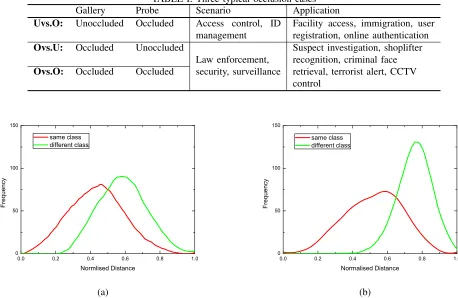
problem [21], and on the other hand, ignore useful information for recognition [20]. We summarise three occlusion cases in Table I, which a FR system may encounter in the real-world applications. Most of the current methods rely on a clean gallery or training set and only consider the first case. The latter two cases would also occur in real environment but have not yet received much attention.

We propose a local matching based method, Dynamic Image-to-Class Warping (DICW), for occluded FR. DICW is motivated by the Dynamic Time Warping (DTW) algorithm [22] which allows elastic match of two time sequences. It has been successfully applied to the area of speech recognition [22]. In our work, an image is partitioned into patches, which are then concatenated in the raster scan order to form a sequence. In this way, a face is represented by a patch sequence which contains the order information of facial fea-tures. DICW calculates the Image-to-Class distance between a query face and those of an enrolled subject by finding the optimal alignment between the query sequence and all enrolled sequences of that subject. Our method allows elastic match in bothtimeandwith-classdirections.

Most of the existing works that simply treat occluded FR as a signal recovery problem or just employ the framework for general object classification, neglect the inherent structure of the face. Wanget al.proposed a Markov Random Field (MRF) based method [23] for FR and confirmed that the contextual information between facial features plays an important role in recognition. In this paper, we propose a novel approach that takes the facial order, which contains the geometry in-formation of the face, into account when recognising partially occluded faces. In uncontrolled environments with uncooper-ative subjects, the occlusion preprocessing and the collection of sufficient and representative training samples are generally very difficult. Our method which performs recognition directly in the presence of occlusions and does not require training, is hence feasible for realistic FR applications.

This paper is built upon our preliminary work reported in [24] and [25]. The remainder of this paper is organised as

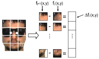
fol-Fig. 1: Image representation of DICW.

lows. The proposed Dynamic Image-to-Class Warping method, from image representation, modelling to implementation, is described in Section II. Extensive experiments including dis-cussions are presented in Section III. Further analysis about why the proposed method works; when and why it will fail and how to improve it is discussed in Section IV. Finally the work is concluded in Section V.

II. DYNAMICIMAGE-TO-CLASSWARPING

A. Image representation

An image is partitioned intoJ non-overlapping patches of

d×d′pixels. Those patches are then concatenated in the raster scan order (i.e., from left to right and top to bottom) to form a single sequence. The reason for doing so is that the forehead, eyes, nose, mouth and chin are located in the face in a natural order, which does not change despite occlusions or imprecise registration. This spatial facial order, which is contained in the patch sequence, can be viewed as the temporal order in the time sequence. In this way, a face image can be viewed as a time sequence so the image matching problem can be handled by the time series analysis technique like DTW [22]. Letf(x, y)be the intensity of the pixel at coordinates(x, y)

andfj(x, y)be the j-patch. A difference patch△fj(x, y) is

computed (Fig. 1) by subtractingfj(x, y)from its immediate

neighbouring patchfj+1(x, y)as:

△fj(x, y) =fj+1(x, y)−fj(x, y) (1)

wherej ∈ {1,2, ..., J−1}. Note that here the length of the

difference patchsequence is J−1.

A difference patch △fj(·) actually can be viewed as the

approximation of the first-order derivative of adjacent patch

fj+1(·)andfj(·). The salient facial features which represent

textured regions such as eyes, nose and mouth can be enhanced since the first-order derivative operator is sensitive to edges.

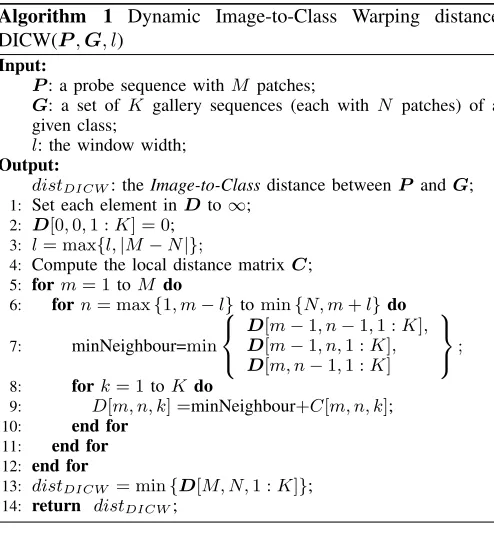
We use 3,200 occluded-unoccluded image pairs of the same class and different classes from the AR database [26], respec-tively (6,400 pairs in total) to calculate the image distance distributions1_{. As shown in Fig. 2, the distance distributions}

of the same and different classes are separated more widely when using the difference patches (Fig. 2b).

1_{We use Euclidean distance as measurement. The image size is83×60}

TABLE I: Three typical occlusion cases

Gallery Probe Scenario Application

Uvs.O: Unoccluded Occluded Access control, ID management

Facility access, immigration, user registration, online authentication Ovs.U: Occluded Unoccluded

Law enforcement, security, surveillance

Suspect investigation, shoplifter recognition, criminal face retrieval, terrorist alert, CCTV control

Ovs.O: Occluded Occluded

0.0 0.2 0.4 0.6 0.8 1.0

0 50 100 150

F

r

e

q

u

e

n

cy

Normlised Distance same class

different class

(a)

0.0 0.2 0.4 0.6 0.8 1.0

0 50 100 150

F

r

e

q

u

e

n

cy

Normalised Distance same class

different class

(b)

Fig. 2: Distributions of face image distance of the same and different classes. Using the difference patch (b), the distance distribution of the same class and that of the different classes are separated more widely compared with those using the original patch (a).

B. Modelling

Face matching is implemented by defining a distance mea-surement between sequences and using the distance as the basis for classification. Generally, a small distance is expected if two sequences are similar to each other. DICW is based on the classical DTW algorithm [22] which is used to compute the distance between two time sequences. Here we use an example to quickly illustrate the main idea of DTW (more details of the algorithm can be found in [22]). As shown in Fig. 3, there are two sequences (each digit indicates a data point):

A=(a1, a2, a3, a4, a5) = (3,1,10,3,2)

B=(b1, b2, b3, b4, b5) = (3,1,2,10,3).

The Euclidean distance (i.e., using point-wise matching, Fig. 3a) between them is √(a1−b1)2_{+...+ (a5}−_b5)2 ₌

√

0 + 0 + 64 + 49 + 1 ≈ 10.68 which is a bit large for these two similar sequences. However, if we warpthese two sequences in a non-linear way by shrinking or expanding them along the time axis during matching (i.e., allows flexible correspondences), the distance between A and B can be largely reduced 2_{to2(Fig. 3b). DTW, which is based on this}

idea, calculates the distance between two time sequences by finding the optimal alignment between them with the minimal overall cost. This will help to reduce the distance error caused

2_{computation details see [22]}

(a)

(b)

(c)

Fig. 3: Various ways of sequence matching. a) Point-wise matching, b) DTW matching, and c) cross matching.

by somenoisedata points and ensure that the distance between similar sequences is relatively small. In addition, thetemporal order is considered during matching, thus cross-matching (which reverses the order of data points) is not allowed even it can lead to shorter distance (Fig. 3c). Especially for FR, this is reasonable since the order of facial features should not be turned back.

the alignment between two sequences, we seek the alignment between a sequence and the sequencesetof a given class (i.e., subject). A probe image consisting of M patch features is denoted by P = (p₁, ...,p_m, ...,p_M). HereP is an ordered list where each element p_m is a patch feature vector (e.g.,

△f(·)in Section II-A). The gallery set of a given class con-taining K images is denoted by G= {G1, ...,Gk, ...,GK}.

The k-th gallery image is similarly represented as a sequence of N patch features as Gk = (g1k, ...,gnk, ...,gN k) where

gnk represents a patch feature vector like pm. Note that the

number of patches in the probe image and that in the gallery image can be different (i.e., the values of M andN can be different) since the DTW model is able to deal with sequences with different lengths [22].

A warping pathW indicating the matching correspondence of patches between P and G with T warping steps in time axis is defined as W = (w(1), ..., w(t), ..., w(T))with:

w(t) = (m, n, k) :

{1,2, ..., T} → {1,2, ..., M} × {1,2, ..., N} × {1,2, ..., K} (2)

where × indicates the Cartesian product operator and

max{M, N}6T 6M +N−1.w(t) = (m, n, k)is a triple indicating that patch p_mis matched to patch g_nk at step t.

Similar to the DTW model [22],W in DICW satisfies the following four constraints:

1) Boundary:w(1) = (1,1, k)andw(T) = (M, N, k′).The path starts at matching p₁ tog_1k and ends at matching

pM togN k′. Note that no restrictions are placed onkand

k′. From step 1 toT,k andk′ can be any value from 1 toK since the probe patch can be matched with patches from all K gallery images.

2) Monotonicity: Given w(t) = (m, n, k), the preceding triple w(t−1) = (m′, n′, k′) satisfies that m′ 6mand

n′ 6n. The warping path preserves the temporal order

and increase monotonically.

3) Continuity: Given w(t) = (m, n, k), the preceding triple

w(t−1) = (m′, n′, k′) satisfies that m−m′ 6 1 and

n−n′ 6 1. The indexes of the path increase by 1 in each step, which means that each step makes smooth transitions along the timedimension.

4) Window constraint: Given w(t) = (m, n, k), it satisfies

|m − n| 6 l where l ∈ N+ is the window width [22]. The window constraint is designed to reduce the computational cost of DICW. But it is also meaningful for the specific FR problem since a probe patch (e.g., eye) should not match to a patch (e.g., mouth) too far away. The window with a widthlis able to constrain the warping path within an appropriate range.

These constraints are extended from the constraints of the DTW algorithm. However, they are also very meaningful in the context of FR with the image representation defined in Section II-A. Our method represents a face image as a patch sequence thus here the image matching problem can be solved by the time series analysis technique.

In order to explain the concept of warping path, we take the aforementioned sequences A and B as an example. In Fig. 4a, each grid on the right hand side indicates a possible matching correspondence. The indexes of the red grids indicate

the matching between A and B by DTW (i.e., the optimal warping path with the minimal matching cost) as shown in the left part (here T = 6). Likewise, the same procedure of DICW is shown in Fig. 4b. Compared with DTW, an additional index is added in the warping step of DICW to index different gallery sequences. In this way, thewarpingis performed in two directions: 1) a probe sequenceP is aligned to a set of gallery sequences G according to the time dimension (maintaining thefacial order) and 2) simultaneously, at each warping step, each patch in P can be matched with any patch among all gallery sequences along the within-class dimension. Our method allows elastic match in both of the aforementioned two directions.

We define the local distance [22]Cm,n,k =d(pm,gnk)as

the distance between two patches p_m and g_nk. d(·) can be any distance measurement such as the Euclidean distance or the Cosine distance. The overall matching cost of W is the sum of the local distance of each warping step:

S(W) =

T

∑

t=1

Cwt (3)

The optimal warping path W∗ (i.e., the red grid path in Fig. 4b) is the path that minimises S(W). The Image-to-Class

distance betweenP andGis simply the overall cost ofW∗:

distDICW(P,G) = min

W

T

∑

t=1

Cwt (4)

After computing distDICW between P and each enrolled

subject in the database, a classifier such as the Nearest Neighbour classifier can be adopted for classification based ondistDICW.

C. Implementation through Dynamic Programming

To compute distDICW(P,G) in (4), one could test every

possible warping path but with a high computational cost. Fortunately, (4) can be solved efficiently by Dynamic Pro-gramming. A three-dimensional matrix D ∈ RM×N×K _is

created to store the cumulative distance. The elementDm,n,k

stores the cost of the optimal warping path of matching the first

m probe patches to the set of firstn patches of each gallery sequence and at the same time them-th patchpmis matched

to the patch from the k-th gallery image. The calculation of the final optimal costdistDICW(P,G)is based on the results

of a series of predecessors. D can be computed recursively as:

Dm,n,k= min   

D_{(m−1,n−1)}×{1,2,...,K},

D_{(m−1,n)}×{1,2,...,K},

D_{(m,n−1)}×{1,2,...,K}

 

+Cm,n,k (5)

where the initialisation is done by extendingDas an(M+1)× (N+1)×Kmatrix and settingD0,0,·= 0,D0,n,·=Dm,0,·=

∞. Thus,distDICW(P,G)can be obtained as follows:

distDICW(P,G) = min k∈{1,2,...,K}{

DM,N,k} (6)

W= ((1,1),(2,2),(2,3),(3,4),(4,5),(5,5)), T= 6 (a)

W= ((1,1,1),(2,1,1),(3,2,2),(4,3,2),(5,4,2),(6,5,1),(7,6,1),(7,7,2),(8,8,1),(9,8,1),(9,9,1),(10,10,1)), T= 12 (b)

Fig. 4: An illustration of warping path in a) DTW and the b) proposed DICW. The arrows indicate the matching correspondence. The dashed line marks the optimal warping path. Black blocks indicate the occluded patches.

Fig. 5: The illustration of a) the Image-to-Image and b) the

Image-to-Classcomparison. Matched features are indicated by the same symbol.

warping path under the temporal constraints then selects the one with minimal overall cost. So the warping path with large distance error will not be selected. The Image-to-Class

distance is the globally optimal cost for matching. Although occlusions are not directly removed, avoiding large distance error by warping is helpful for classification from our experi-mental results (see Section III).

In addition, a patch of the probe image can be matched to patches of K different gallery images of the same class. Because the chance that all patches at the same location of the

K images are occluded is low, the chance that a probe patch is compared to an unoccluded patch at the same location is thus higher. When occlusions occur in probe or/and gallery images, theImage-to-Image distance may be large. However, our model is able to exploit the information from different gallery images and reduce the effect of occlusions (Fig. 5). Algorithm 1 summarises the procedure of computing the

Image-to-Classdistance between a probe image and a class.l

is the window width and usually set to 10%of max{M, N}

[22]. Computational complexity is analysed in Section III-D6.

Algorithm 1 Dynamic Image-to-Class Warping distance DICW(P,G, l)

Input:

P: a probe sequence withM patches;

G: a set ofK gallery sequences (each withN patches) of a given class;

l: the window width;

Output:

distDICW: theImage-to-Classdistance betweenP andG; 1: Set each element inDto∞;

2: D[0,0,1 :K] = 0;

3: l= max{l,|M−N|};

4: Compute the local distance matrixC; 5: form= 1toM do

6: forn= max{1, m−l}tomin{N, m+l}do

7: minNeighbour=min

  

D[m−1, n−1,1 :K],

D[m−1, n,1 :K],

D[m, n−1,1 :K]

  ; 8: fork= 1to Kdo

9: D[m, n, k] =minNeighbour+C[m, n, k]; 10: end for

11: end for 12: end for

13: distDICW= min{D[M, N,1 :K]};

14: return distDICW;

III. EXPERIMENTALANALYSIS

situation that occlusions exist in gallery images, which is a case most of the current works do not take account. We fix the number of gallery images per subject and conduct experiments step by step: firstly the probe images are not occluded (i.e., Ovs.U); and then both the gallery and probe images are occluded (i.e.,Ovs.O). Note that, for comparison purpose, the experiments on the FRGC and the AR databases also include the case that no occlusion is presented in both gallery and probe images to confirm that DICW is also effective in general conditions. In addition, we also extend DICW to verification tasks with faces containing large uncontrolled variations.

Note that in all experiments, the gallery image set is disjoint with all probe sets. Considering that the gallery and probe images are at the same scale, in the experiments, the probe images and the gallery images are partitioned into the same number of patches, i.e., M =N as defined in Section II-B. As recommended in the work [30], the Euclidean distance and the Cosine distance are used as local distance measurements for the pixel intensity feature and the LBP feature [31], respectively.

We quantitatively compare DICW with some representative methods in the literature: the supervised linear SVM [32] using PCA [33] for feature extraction (PCA+LSVM), the reconstruc-tion based SRC [8] as introduced in Secreconstruc-tion I, the Image-to-Classdistance based Naive Bayes Nearest Neighbour (NBNN) [34] as ours, and the baseline, Hidden Markov models (HMM) [35] which also considers the order information in a face. We use the difference patch representation as defined in Section II-A in NBNN and DICW. For comparison purpose, we also report the results of using the original patche (referred to OP-NBNN and OP-Warp, respectively).

Note that NBNN is a local patch based method which also exploits the Image-to-Classdistance. But it does not consider the spatial relationship between patches like ours. To improve the performance, a location weight α [34] is used in NBNN to constrain matching patches according to their locations. We tested different values ofαand found that the performance of NBNN is highly dependent on the value of α and different testing data (e.g., different occlusion level, location) requires different value even within the same database. So we also reported the best result for each test with the optimal αvalue (as NBNN-ub and NBNN-ub). The performance of OP-NBNN-ub and OP-NBNN-ub can be seen as the upper bound of the performance of NBNN, which is a competitive comparison for DICW.

A. Face identification with randomly located occlusions

We first evaluate the proposed method using the Face Recognition Grand Challenge (FRGC) database [27] with randomly located occlusions. Note that in each image, the locations of occlusions are randomly chosen and unknown to the algorithm. Especially, in theOvs.Oscenario, the locations of occlusions in the gallery images are different from those in the probe images. We use these images with randomly located occlusions to evaluate the effectiveness of DICW when there is no prior knowledge of the occluded location.

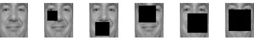
The FRGC database contains 8,014 images from 466 sub-jects in two sessions. These images contain variations such as

Fig. 6: Sample images from the FRGC database with randomly located occlusions.

illumination and expression changes, time-lapse, etc. Similar to the work in [7], an image set of 100 subjects (eight images in two sessions are selected for each subject), is used in experiments. To simulate the randomly located occlusions, we create an occluded image set by replacing a randomly located square patch (size of 10% to 50% of the original image) from each image in the original image set with a black block (Fig. 6). We design experiments according to the three occlusion scenarios:Uvs.O,Ovs.U andOvs.O. There are 2,400 testing samples for each scenario. All images are cropped and re-sized to80×65pixels and the patch size is6×5 pixels (the effect of patch size is discussed in Section III-D1).

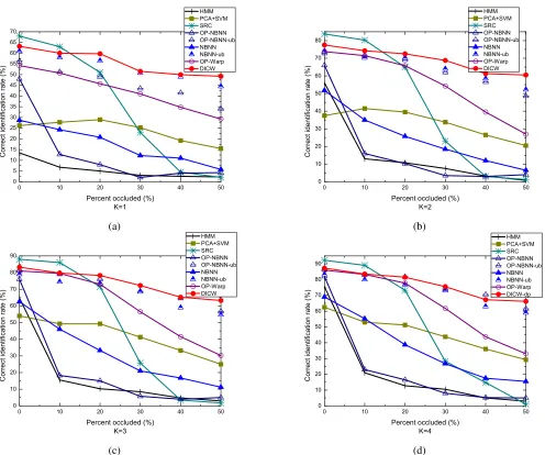
Uvs.O: For each subject, we select K = 1,2,3 and 4

unoccluded images respectively to form the gallery sets and use the other four images with synthetic occlusions as the probe set. Fig. 7 shows the recognition results with different values of K. The correct identification rates of all methods increase when more gallery images are available (i.e., greater value of K). When there are multiple gallery images per class and no occlusion (level=0%) in images, HMM performs better than the supervised method SVM and the local matching based NBNN. But its performance is significantly affected by the increasing occlusions. In addition, when K = 1, HMM performs worst among all methods since there are not enough gallery images to train a HMM for each class. For NBNN and DICW, using the difference patch achieves better results than using the original patch (i.e., OP-NBNN and OP-Warp). Especially, by comparing DICW with OP-Warp, and NBNN with OP-NBNN, it can be found that difference patches improve the results of DICW more significantly than that of NBNN. As introduced in Section II-A, the difference patches are generated by the spatially continuous patches so they enhance the order informationwithin a patch sequence, which is compatible with DICW. With the optimal location weights, NBNN-ub and OP-NBNN-ub perform better than SVM. When K = 1,2,3 and 4, the average rates for the six occlusion levels of DICW are 2.3%, 4.3%, 5.5% and 4.4% better than that of NBNN-ub, respectively. When the occlusion level = 0%, the performance of SRC is better than DICW. However, the performance drops sharply when the degree of occlusion increases. WhenK= 1, theImage-to-Classdistance degenerates to the Image-to-Image distance. DICW, which allows time warping during matching, still achieves better results while the level of occlusion increases.

0 10 20 30 40 50 0 5 10 15 20 25 30 35 40 45 50 55 60 65 70 C o r r e ct i d e n t i f i ca t i o n r a t e ( % )

Percent occluded (%) K=1 HMM PCA+SVM SRC OP-NBNN OP-NBNN-ub NBNN NBNN-ub OP-W arp DICW (a)

0 10 20 30 40 50

0 10 20 30 40 50 60 70 80 C o r r e ct i d e n t i f i ca t i o n r a t e ( % )

Percent occluded (%) K=2 HMM PCA+SVM SRC OP-NBNN OP-NBNN-ub NBNN NBNN-ub OP-W arp DICW (b)

0 10 20 30 40 50

0 10 20 30 40 50 60 70 80 90 C o r r e ct i d e n t i f i ca t i o n r a t e ( % )

Percent occluded (%) K=3 HMM PCA+SVM SRC OP-NBNN OP-NBNN-ub NBNN NBNN-ub OP-W arp DICW (c)

0 10 20 30 40 50

0 10 20 30 40 50 60 70 80 90 C o r r e ct i d e n t i f i ca t i o n r a t e ( % )

Percent occluded (%) K=4 HMM PCA+SVM SRC OP-NBNN OP-NBNN-ub NBNN NBNN-ub OP-W arp DICW -dp (d)

Fig. 7:Uvs.O: identification results on the FRGC database with different number of gallery images (K) per subject.

as the probe set (Ovs.O). Note that the images in the gallery set are different from those in the probe sets. Fig. 8 shows the recognition results. The methods (e.g., HMM, SVM, SRC) which include occluded gallery images for training/modelling perform poorly in these two cases. NBNN does not perform consistently in Ovs.U and Ovs.O. Using the original patch (i.e., OP-NBNN) performs better than using the difference patch (i.e., NBNN) inOvs.U. For DICW, using the difference patch is always better than using the original patch (i.e., OP-Warp). This confirms that the difference patch works better with DICW, as analysed before. DICW outperforms the best of NBNN (i.e., NBNN-ub) by a larger margin of 5.5% (Fig. 8a) and 8.1% (Fig. 8b) on average than that (4.4% in Fig. 7d) in the Uvs.O tested with K = 4. These results confirm the effectiveness and robustness of DICW when the gallery and probe images are occluded. On the whole, our method performs consistently and outperforms other methods in all three occlusion cases.

B. Face identification with facial disguises

We next test the proposed method on the AR database [26] which contains real occlusions. First, we consider that no occlusion is present in both gallery and probe sets. Next, we conduct experiments according to the three occlusion cases. DICW does not rely on the prior knowledge of occlusions. We will demonstrate that it works well in both general and difficult situations later.

The AR database contains over 4,000 colour images of 126 subjects’ faces. For each subject, 26 images in total are taken in two sessions (two weeks apart). These images suffer from different variations in facial expressions, illumination conditions and occlusions (i.e., sunglasses and scarf, as shown in Fig. 5). Similar to the works in [7], [8], [6], [20], [36], [37], a subset of the AR database (50 men and 50 women) is used [38]. All images are cropped and re-sized to 83×60 pixels and the patch size is 5×5 pixels.

0 10 20 30 40 50 0

10 20 30 40 50 60 70 80 90

C

o

r

r

e

ct

i

d

e

n

t

i

f

i

ca

t

i

o

n

r

a

t

e

(

%

)

Percent occluded (%) HMM

PCA+SVM SRC OP-NBNN OP-NBNN-ub NBNN NBNN-ub OP-W arp DICW

(a)

0 10 20 30 40 50

0 10 20 30 40 50 60 70 80 90

C

o

r

r

e

ct

i

d

e

n

t

i

f

i

ca

t

i

o

n

r

a

t

e

(

%

)

Percent occluded (%) HMM PCA+SVM SRC OP-NBNN OP-NBNN-ub NBNN NBNN-ub OP-W arp DICW

(b)

Fig. 8: a)Ovs.U and b)Ovs.O: identification results on the FRGC database with occlusions in gallery or/and probe sets.

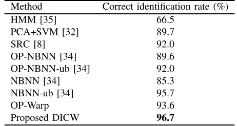
the experiments). In this section, we adopt the setting in [8] using images without occlusions to further test DICW. For each subject, 14 images are chosen (four neutral faces with different illumination conditions and three faces with different expressions in each session). Seven images from Session 1 are used as the gallery set and the other seven from Session 2 as the probe set. Table II shows the identification rates. HMM does not perform as good as others. This may be due to other variations such as illumination and expression changes in the training images. Again, the difference patch does not improve NBNN comparing with the original patch (i.e., OP-NBNN). With the optimal location weights, the difference patch (i.e., NBNN-ub) is 3.7% better than the original patch (i.e., OP-NBNN-ub). For DICW, using the difference patch is 3.1% better than using the original patch (OP-Warp). As analysed in Section III-A, the difference patch can enhance the relative order of adjacent patches, the results in Table II also indicates that the difference patch is more compatible with these methods which considers the order information. When there is no occlusion in the gallery and probe images, both reconstruction based method (e.g., SRC) and local matching based methods (e.g., NBNN and DICW) achieve relatively satisfactory results. DICW significantly outperforms NBNN and is still slightly better than the upper bound of NBNN (i.e., NBNN-ub).

Uvs.O: The unoccluded frontal view images with various expressions are used as the gallery images (eight images per subject). For each subject, we select K = 1,2,4,6 and 8

images to form the gallery sets, respectively. Two separate image sets (200 images each) containing sunglasses (cover about 30% of the image) and scarves (cover about 50% of the image) respectively are used as probe sets. Fig. 9 shows the recognition results. The correct identification rates increase when more gallery images are available. HMM and SVM are generic training based methods and are unable to deal with

unseenocclusions in the probe images. In the scarf testing set, the performance of SRC deteriorates significantly compared

with that on the sunglasses set due to the occluded area is much larger. Local matching based NBNN and DICW perform better than others on the whole. With the optimal location weights, NBNN-ub achieves very comparable performance to DICW. But DICW is slightly superior. Even atK= 1, DICW still achieves 90% and 83% on the sunglasses set and scarf set, respectively.

With the same experimental setting, we also compare DICW with the state-of-the-art algorithms (using eight gallery images per subject, K = 8). The results are shown in Table III. Only the pixel intensity feature is used except the MLERPM method. MLERPM, which is also a local matching based method as ours, uses SIFT [39] and SURF [40] features to handle the misalignment of images. Note that compared with other methods, DICW does not require training. It achieves comparable or better recognition rates among these methods and with a relatively low computational complexity (see Sec-tion III-D6). In the scarf set, albeit the fact that nearly half of the face is occluded, only 2% images are misclassified by DICW. To the best of our knowledge, this is the best result achieved on the scarf set under the same experimental setting. Ovs.U andOvs.O: For theOvs.U scenario, we select four images with sunglasses and scarves to form the gallery set

TABLE II: Identification results on the AR database without occlusions (K=7)

Method Correct identification rate (%)

HMM [35] 66.5

PCA+SVM [32] 89.7

SRC [8] 92.0

OP-NBNN [34] 89.6

OP-NBNN-ub [34] 92.0

NBNN [34] 85.3

NBNN-ub [34] 95.7

OP-Warp 93.6

1 2 3 4 5 6 7 8 20 30 40 50 60 70 80 90 100 C o r r e ct i d e n t i f i ca t i o n r a t e ( % )

The number of gallery image per person K Sunglasses set HMM PCA+SVM SRC OP-NBNN OP-NBNN-ub NBNN NBNN-ub OP-W arp DICW (a)

1 2 3 4 5 6 7 8

10 20 30 40 50 60 70 80 90 100 C o r r e ct i d e n t i f i ca t i o n r a t e ( % )

The number of gallery image per person K Scarf set HMM PCA+SVM SRC OP-NBNN OP-NBNN-ub NBNN NBNN-ub OP-W arp DICW (b)

Fig. 9:Uvs.O: identification results on the AR database with a) sunglasses occlusion and b) scarf occlusion.

TABLE III: Uvs.O: comparison of DICW and the-state-of-the-art methods (K=8)

Method Sunglasses Scarf Average Feature

SRC-partition1[8] 97.5 93.5 95.5

Greyscale

LRC [9] 96.0 26.0 61.0

CRC-RLS-partition1[11] 91.5 95.0 93.3

SEC-MRF [41] 99.0∼100 95.0∼97.5 97.0∼98.8

lstruct [36] 99.5 87.5 93.5

OP-Warp 97.5 95.0 96.3

Proposed DICW 99.5 98.0 98.8

MLERPM [37] 98.0 97.0 97.5 SIFT [39]&SURF [40]

1_{SRC-partitionandCRC-RLS-partitionindicate the strategy of partitioning an image into4×2patches for}

performance improvement for the original method SRC [8] and CRC-RLS [11], respectively.

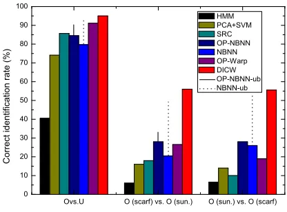
and eight unoccluded images as the probe set. For the Ovs.O scenario, we conduct two experiments: 1) two images with scarves as the gallery set and two images with sunglasses as the probe set; 2) vice versa. Note that with this setting, in each test the occlusion type in the gallery set isdifferent from that in the probe set, which is very challenging for recognition.

The results are shown in Fig. 10. On the gallery set which contains occluded faces, the results of HMM and SVM are much worse than others as expected. In the Ovs.O testing, there are only two gallery images per subject. It is very difficult for SRC to reconstruct an unoccluded probe image with such limited number of gallery images. Local matching based NBNN and DICW perform better. Comparing OP-NBNN with OP-OP-NBNN-ub, and OP-NBNN with OP-NBNN-ub, it can be found that the performance of NBNN is highly dependent on the optimal location weights. Overall, DICW consistently outperforms the best of NBNN (i.e., NBNN-ub) by about 4% on average.

C. Face identification with general occlusions in realistic environment

In this Section, we test our method on the The Face We Make (TFWM) [28] database captured under natural and arbitrary conditions. It has more than 2,000 images which contains frontal view faces of strangers on the streets with un-controlled lighting. The sources of occlusions include glasses,

Ovs.U O (scarf) vs. O (sun.) O (sun.) vs. O (scarf) 0 10 20 30 40 50 60 70 80 90 100 HMM PCA+SVM SRC OP-NBNN NBNN OP-W arp DICW OP-NBNN-ub NBNN-ub C o r r e ct i d e n t i f i ca t i o n r a t e ( % )

Fig. 10: Ovs.U and Ovs.O: identification results on the AR database with occlusions in gallery or/and probe sets.

sunglasses, hat, hair and hand on the face. Besides occlusions, these images also contain expression, pose and head rotation variations. In our experiments, we use images of 100 subjects (ten images per subject) containing various types of occlusions (Fig. 11). For each subject, we choose K = 1,3,5 and

Fig. 11: Sample images from the TFWM database.

1 2 3 4 5 6 7 8

10 20 30 40 50 60 70 80

C

o

r

r

e

ct

i

d

e

n

t

i

f

i

ca

t

i

o

n

r

a

t

e

(

%

)

Number of gallery images per person K HMM SRC PCA+SVM OP-NBNN OP-NBNN-ub NBNN NBNN-ub OP-W arp DICW

Fig. 12: Identification rates (%) on the TFWM database.

remaining two images as the probe set. Occlusions occur at random in the gallery or probe set or in both. This includes all the three occlusion scenarios in Section I. The face area of each image is cropped from the background and re-sized to80×60pixels and the patch size is 5×5pixels. Only the pixel intensity feature is used in all methods.

The recognition results are shown in Fig. 12. Note that the images used in the experiments are not well aligned due to the uncontrolled variations. Some occlusions (e.g., hand) have very similar texture as the face, which are difficult to be detected by skin colour based models [42]. NBNN, which only relies on the texture similarity without considering the structural constraint of a face, does not achieve comparable performance as ours. As more gallery images are available, the accuracies of all methods increase. When K = 8, most methods reach abottleneck with the rate around 65%. DICW outperforms these methods by a notable margin.

D. Discussion

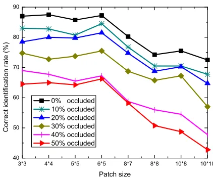
1) The effect of patch size: To investigate this the impact of patch size on the performance, we use 400 unoccluded images (size of80×65pixels) of 100 subjects from the FRGC database as the gallery set and 400 images in each of six probe sets, which contain randomly located occlusions from 0% to 50% level, respectively. We test DICW with the patch sizes from 3×3 pixels to 10×10 pixels. Note that we employ this dataset because the location and size of the occlusions is independent to the patch size.

The correct identification rates with respect to the patch size are shown as Fig. 13. There is no sharp fluctuation in each

3*3 4*4 5*5 6*5 8*7 8*8 10*8 10*10 40

50 60 70 80 90

C

o

r

r

e

ct

i

d

e

n

t

i

f

i

ca

t

i

o

n

r

a

t

e

(

%

)

Patch size 0% occluded

10% occluded 20% occluded 30% occluded 40% occluded 50% occluded

Fig. 13: Identification rates (%) with respect to the patch size.

of the rate curve when the patch size is less than or equal to6×5 pixels. Our method is robust to different patch sizes in an appropriate range despite the ratio of occlusions. The relatively smaller patches lead to better recognition rate since they provide more flexibility to use spatial information than the larger ones. Based on the experimental results, sizes smaller than6×5pixels are recommended.

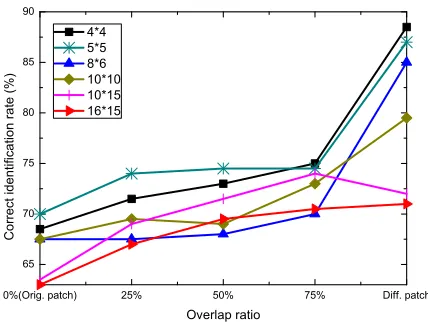
2) The effect of patch overlap: In the previous experiments we used the difference patch to enhance the textured features in patches. It is interesting to see if the overlapping patch has this similar effect. We conducted experiments on the AR database to investigate this since it contains real occlusions with different textures. We selected four unoccluded images from Session 1 for each subject as the gallery set and two im-ages with sunglasses and scarves from Session 2 as the probe set so the testing dataset contains variations of occlusions and illumination changes. We tested the use of different patch sizes (4×4to16×15pixels) with different overlap ratios (0%, 25%, 50%, 75%) and compared their results with that of using the difference patch. 25% ratio means the adjacent patches have a 25% horizontal overlap. So the larger the ratio is, the larger the number of patches will be in each image sequence. Note that 0% overlap ratio means using the original patches (with intensity features).

0%(Orig. patch) 25% 50% 75% Diff. patch 65

70 75 80 85 90

C

o

r

r

e

ct

i

d

e

n

t

i

f

i

ca

t

i

o

n

r

a

t

e

(

%

)

Overlap ratio 4*4

5*5 8*6 10*10 10*15 16*15

Fig. 14: Identification rates (%) with respect to the overlap ratio comparing with using the difference patches.

texture in a large patch is less uniform. Note that the overall performance of using the small patch is better than that of using the large patch. DICW is compatible with the small patch as analysed in Section III-D1 so in the experiments we used the best one, the difference patch instead of the overlapping patch.

3) The effect of image descriptor: In Section III-D2, our experiments indicate that the difference patch leads to better accuracy since it is able to enhance the textured regions in a face image. In this section we will carry out experiments to compare the discriminative power of the proposed difference patches and other local image descriptors such as 2D-DCT (Discrete Cosine Transform coefficients), Gabor [43], LBP [31] and dense SIFT [44]. We use the same dataset in Section III-D2 and test both small patch size (i.e., 5×5 pixels) and large patch size (i.e., 16×15pixels).

Fig. 15 shows the recognition results. The 2D-DCT feature is not as discriminative as others so it performs worst. For large patch size, as we analysed before, the difference patch does not perform very well. For small patches, the performance of difference patch is comparable with that of SIFT and LBP. The Gabor features do not perform better than the difference patch since the patch is too small to extract discriminative features. Note that the computation of difference patch is much simpler than other images descriptors. From Fig. 15 we can see, the local image descriptor is able to strengthen DICW when the image contains uncontrolled variations such as illumination changes and occlusions. When dealing with the uncontrolled data, applying these local features can further improve the performance of DICW.

4) Robustness to misalignment: The face registration error can largely degrade the recognition performance [1] as we mentioned in Section I. To evaluate the robustness of DICW to the misalignment of face images, we use a subset of the AR database with 110 subjects (referred to AR-VJ) used in the work in [45]. The faces in AR-VJ are automatically detected by the Viola & Jones detector [46] and cropped directly from the images without any alignment. Different from the images

5*5 (small) 16*15 (large) 60

65 70 75 80 85 90 95

C

o

r

r

e

ct

i

d

e

n

t

i

f

i

ca

t

i

o

n

r

a

t

e

(

%

)

Patch size

2D-DCT Gabor dense SIFT LBP Diff. patch

Fig. 15: Identification rates (%) of using different image descriptors and the difference patches.

Fig. 16: Sample images of the same subject from the AR database without alignment (AR-VJ).

in the original AR database which are well cropped (Fig. 5), these images contain large crop and alignment errors as shown in Fig. 16.

Following the same experimental setting in [45], seven images of each subject from the first session are used as the gallery set and the other seven images from the second session as the probe set. All images are re-sized to65×65pixels and the patch size is5×5pixels. As analysed in the last section, we use the LBPu2

8,2 descriptor [31] for feature extraction to

handle the illumination variations.

The recognition results are shown in Table IV. DICW outperforms other methods and achieves very close result to P2DW-FOSE [45], which is also a training-free method like ours. But different from DICW, which performs warping on thepatch level, P2DW-FOSE is a pseudo 2D warping method on thepixel level and its time complexity is quadratic in the number of pixels [45].

TABLE IV: Identification rate (%) on the AR-VJ dataset Method Correct identification rate (%)

Av-SpPCA1[47] 93.6

DCT1[1] 95.3

SURF-Face [48] 95.9

P2DW-FOSE [45] 98.2

Proposed DICW 97.3

1 _{Using manually aligned images}

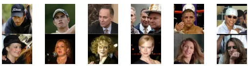
Fig. 17: Sample images from the LFW database (six matched image pairs for six subjects).

Faces in the Wild (LFW) database [29], which is the most active benchmark for FR. The task of face verification under the LFW database’s protocol is to determine if a pair of face images belongs to the same subject or not. Note that in the verification of each pair, it is a Image-to-Image comparison. So the experiments on the LFW database can be considered as an evaluation for the effectiveness of DICW when only time warpingis used (nowithin-class warping).

The LFW database contains 13,233 face images of 5,749 subjects collected from the Internet. These images are captured in uncontrolled environments and contain large variations in pose, illumination, expression, time-lapse and various types of occlusions (Fig. 17). Following the testing protocol of View 2, we use the most difficult experimental setting: restrict-ed unsupervisrestrict-ed setting where no class label information is available. In View 2, there are 3,000 matched (i.e., positive) and 3,000 mismatched (i.e., negative) image pairs. They are equally divided into ten randomly generated sets and the final verification performance is evaluated by the ten-fold cross-validation. Here image pairs are classified intothe same subject ordifferent subjectsby thresholding on their distance. We use the LFW-a version and LBPu_8,2₂ as feature descriptor. All images are cropped and re-sized to 150×80 pixels and the patch size is3×3 pixels.

Chenet al.’s work [49] produces very competitive results on the LFW database by using the high-dimensional LBP feature. It is confirmed that features sampled at facial landmarks lead to better recognition performance than those sampled from regular grids. Motivated by this, we also select 25 landmarks [50] of the inner face and follow the similar process as in [49]: 1) normalise the unaligned images according to 2 facial landmarks (i.e., the tip of the nose and the centre of the mouth), and 2) extract image blocks (size of 30×30

pixels) centred around 25 facial landmarks from each image. Each block is partitioned into 3×3pixels patches which are then concatenated to form a sequence. The original DICW algorithm is performed according to each block (i.e., sequence) and a corresponding distance is generated respectively. The sum of these distances is the final distance for each image pair. We refer our method with this strategy (i.e., sampling features around landmarks) as DICW-L and the original DICW (i.e., sampling features from regular grids) as DICW-G.

LFW is an extremely challenging database containing large uncontrolled variations, especially pose changes. As presented in [51], the first several principal components (PCs) usually capture these uncontrolled variations in the principal compo-nent analysis (PCA) subspace [33]. Therefore, we adopt the component analysis process in [51] to remove the first several

Fig. 18: ROC curves of the-state-of-the-art methods and DICW on the LFW database.

PCs for performance improvement by:

F′ =F −XiXTiF (7)

where F is the original feature vector of an image by con-catenating all the patch features of the image sequence (i.e.,

P or Gk in Section II-B) and Xi is the first i components

in the PCA subspace. We quantitatively test the value of i

using the View 1 dataset provided by the LFW database and set the optimal valuei= 8.F′ is the improved feature vector used in the experiments for the LFW database. In this way, the large uncontrolled variations can be reduced to some extent. At the same time, different from the general dimension reduction operation (i.e., the original PCA), the topological structure of each image is still maintained so our patch based DICW can be performed directly on the improved features by this process.

We compare DICW with other methods under the same test-ing protocolwithout outside training data. In the experiments, only LBPu8,22 descriptor [31] is used. We draw the the ROC

(Receiver Operating Characteristic) curves of DICW and other state-of-the-art methods in Fig. 18. It shows the performance of DICW-G is better than other methods which use only single feature such as SD-MATCHES (SIFT [39]), H-XS-40 (LBP [31]), GJD-BC-100 (Gabor [43]), LARK (locally adaptive regression kernel descriptor [52]) and LHS (local higher-order statistics [53]). When extracting features around facial landmarks, the performance of DICW is further improved with a large margin. The area under the ROC curve (AUC) of DICW-L is 0.874 as shown in Table V, which is the best among all methods. These experimental results confirm the effectiveness of DICW even onlytime warpingis performed.

6) Computational complexity and usability analysis: From Algorithm 1 in Section II-C we can see that the time com-plexity of DICW for computing the distance between a query image and an enrolled class is O(max{M, N}lK), where

M′ to representmax{M, N}. The number of gallery images per classKis very small compared with the number of patches

M′ in each sequence (i.e., K ≪ M′). Thus the complexity is represented as O(M′l). Note that usually l = 10%M′, so the warping distance can be obtained very efficiently. On the other hand, the computational cost of the reconstruction based method SRC is very high [8]. To facilitate intuitive comparisons, Table VI shows the runtime of DICW and SRC

3 _{for classifying a query image under the same setting as}

the experiments of Table III using Matlab implementation (running on a platform with quad-core 3.10GHz CPUs and 8 GB memory). DICW is about 15 times faster than SRC [8] when classifying a query image.

Compared with the reconstruction based approaches, which represent a query image using all enrolled images, DICW computes the distance between the probe image and each enrolled class independently. So in the real FR applications, the distance matrix can be generated in parallel and the enrolled database can be updated incrementally. This is very practical for the real-world applications.

IV. FURTHER ANALYSIS AND IMPROVEMENT

In the previous sections, we evaluate DICW using exten-sive experiments with face images with various uncontrolled variations. In this section we will further analysis why the DICW works compared with similar methods, and when and why it will fail. We also discuss the idea for improving the performance of DICW.

NBNN [34] presented in the previous sections is a similar method to ours. It also calculates theImage-to-Classdistance between a probe patch set and a gallery patch set from a given class. The difference is that it does not consider the spatial relationship between patches like ours and each probe patch can be matched to any patches from any location in the gallery patch set. Fig. 19 is an illustration example. The occluded probe image is from class 74 but is incorrectly classified to the class 5 by NBNN. Actually the images from class 74 and class

3_{We use thel1 lspackage for implementation. http://www.stanford.edu/}

∼boyd/l1 ls/

TABLE V: Area under ROC curve (AUC) on the LFW database under unsupervised setting.

Method AUC Feature extraction SD-MATCHES [54] 0.5407

From grids H-XS-40 [54] 0.7574

GJD-BC-100 [54] 0.7392

LARK [52] 0.7830

LHS [53] 0.8107

Proposed DICW-G 0.8286

Proposed DICW-L 0.8740 From landmarks

TABLE VI: Comparison of average runtime (s) Per class All class

SRC [8] N/A 89

Proposed DICW 0.05 6

(a) (b) (c)

5 101520253035404550556065707580859095100

Class 5 (wrong)

N

o

m

a

li

se

d

d

i

st

a

n

ce

Class index

(d) By NBNN

5 101520253035404550556065707580859095100

N

o

m

a

l

ise

d

d

ist

a

n

ce

Class index

Class 74 (correct)

(e) By DICW

Fig. 19: a) The probe image from class 74. b) Classification result (class 5) by NBNN. c) Classification result (class 74) by DICW. Distance to each class computed by d) NBNN and by e) DICW.

5 are not alike. But the texture of sunglasses is very similar to that of beard in class 5. Without the location constraint, the beard patches are wrongly matched to the sunglasses thus the distance is affected by this occlusion. On the other hand, DICW keeps the order information and matches patches within a proper range which leads to correct classification.

(a) (b) (c)

Fig. 20: a) A probe image from class 51. b) The wrong class (class 72) classified by DICW. c) The gallery image from class 51.

for practical applications. In DICW, the order constraint is naturally encoded during distance computation.

DICW represents a face image as a patch sequence which maintains the facial order of a face. To some extent, the geometric information of a face is reduced from 2D to 1D. However, the direct 2D image warping is an NP-complete problem [55]. P2DW-FOSE mentioned in Section III-D4 is a pseudo 2D warping method but with a remarkably large computational cost (i.e., quadratic in the number of pixels) [45]. DICW incurs a lower computational cost due to its patch sequence representation. In addition, each patch still contains the local 2D information which is helpful for classification.

Improving the performance with random selection and majority voting scheme Fig. 20 shows a fail example which can not be correctly classified by both DICW and NBNN. The discriminative eyes region is occluded by sunglasses, which makes recognition difficult. In addition, a probe face with sunglasses (Fig. 20a) is more similar to a gallery face with glasses (Fig. 20b) in the feature space, which leads to misclassification.

Looking back to the definition of DICW in Section II-B, although warping is helpful for avoiding large distance error caused by occlusions, the occluded area is not directly re-moved during matching. Here we employ a simple but very effective scheme for improving the performance of DICW. As shown in Fig. 21, we do not use all patches in a probe sequence for warping, instead, we randomly select a subset of patch set then compute theImage-to-Classdistance based on this subset. We repeat thisntimes and generate a class label (the class with the shortest distance) each time according to the calculated distance. Finally, the final class label is decided by majority voting by n experts. With random selection, it is possible to skip the occluded patches. It is also possible that the occluded patches are chosen but this effect will be eliminated by the majority voting strategy since we assume that the occluded areas only take up a small part of a face. This assumption is reasonable since if most parts of a face are occluded, even a human being will feel difficult to recognise it. Different from theocclusion detectionbased methods which attempt to detect and remove occlusion area as we mentioned before, this simple strategy does not rely on any prior knowledge nor any data-dependent training.

Here we use the same setting to Section III-D2. We random-ly select 15% patches in a sequence each time as anexpertand select n= 50 expertsin total. Since this scheme is based on random selection, we repeat the whole classification process ten times and calculate the average identification rate. The results are shown in Table VII. The performance of DICW is improved by 2% on average by using only 50experts (Note

Fig. 21: Random selection and majority voting scheme for improving the performance of DICW.

that for eachexpert, the computation of DICW is much faster than before since the number ofsubsetpatches is much smaller than that of the whole sequence). Generally, more experts will lead to higher accuracy since this increases the diversity of decision views, which is more robust to different variations. But this will also raise the whole computational cost, which needs to be considered to keep a balance between accuracy and computation. The improvement is more obvious when the number of image per class is limited. A preliminary study of using this scheme to improve DICW whenK= 1is discussed in [56].

TABLE VII: Identification rates (%) of DICW and the im-provement scheme on the AR database.

# Img./class (K) 1 2 3 4

DICW 81.0 83.5 86.0 87.0

Improvement scheme 84.5 85.2 86.5 89.0

V. CONCLUSION AND FUTURE WORK