http://go.warwick.ac.uk/lib-publications
Original citation:
Elliott, Charles M., Stinner, Björn and Venkataraman, Chandrasekhar. (2012) Modelling
cell motility and chemotaxis with evolving surface finite elements. Journal of The Royal
Society Interface, Vol.9 (No.76). pp. 3027-3044. ISSN 1742-5689
Permanent WRAP url:
http://wrap.warwick.ac.uk/52273
Copyright and reuse:
The Warwick Research Archive Portal (WRAP) makes the work of researchers of the
University of Warwick available open access under the following conditions. Copyright ©
and all moral rights to the version of the paper presented here belong to the individual
author(s) and/or other copyright owners. To the extent reasonable and practicable the
material made available in WRAP has been checked for eligibility before being made
available.
Copies of full items can be used for personal research or study, educational, or
not-for-profit purposes without prior permission or charge. Provided that the authors, title and
full bibliographic details are credited, a hyperlink and/or URL is given for the original
metadata page and the content is not changed in any way.
Publisher’s statement:
http://dx.doi.org/10.1098/rsif.2012.0276
A note on versions:
The version presented here may differ from the published version or, version of record, if
you wish to cite this item you are advised to consult the publisher’s version. Please see
the ‘permanent WRAP url’ above for details on accessing the published version and note
that access may require a subscription.
FINITE ELEMENTS
CHARLES M. ELLIOTT, BJ ¨ORN STINNER, AND CHANDRASEKHAR VENKATARAMAN
ABSTRACT. We present a mathematical and computational framework for the modelling of cell motility. The cell membrane is represented by an evolving surface, with the movement of the cell determined by the interaction of various forces that act normal to the surface. We consider external forces such as those that may arise due to inhomogeneities in the medium and a pressure that constrains the enclosed volume, as well as internal forces that arise from the reaction of the cells surface to stretching and bending. We also consider a protrusive force associated with a reaction-diffusion system posed on the cell membrane, with cell polarisation modelled by this surface reaction-diffusion system. The computational method is based on an evolving surface finite element method. The general method can account for the large deformations that arise in cell motility and allows the simulation of cell migration in three dimensions. We illustrate applications of the proposed modelling framework and numerical method by reporting on numerical simulations of a model for eukaryotic chemotaxis and a model for the persistent movement of keratocytes in two and three space dimensions. Movies of the simulated cells can be obtained fromhttp://homepages.warwick.ac. uk/˜maskae/CV_Warwick/Chemotaxis.html
Keywords: cell motility, chemotaxis, surface finite elements, reaction diffusion systems
1. INTRODUCTION
Modelling the directional motility of cells is of much importance especially due to the central role directed cell migration plays in several biological phenomena such as embryonic development, cancer, tissue development and immune responses [1]. Broadly speaking the motile cycle of a cell consists of the following processes: polarisationwhere the cell develops a front and a back through the redistribution of proteins and lipids within the cell,protrusionat the leading edge of the cell pushing the front of the cell outwards andretractionof the rear of the cell towards the leading edge [2]. Although the main as-pects of the motile cycle appear deceptively simple, as further details are added to the modelling various complexities arise. For example in the case of chemotactic eukaryotic cells, the molecular mechanisms that govern gradient sensing and cell polarisation are still not fully understood [3]. Furthermore, it is difficult to quantify the forces associated with motility and only recently has experimental progress been made in this direction [4, 5]. Direct numerical simulation of cell motility necessitates the consideration of deformable surfaces [6, 7] or multi-phase flow models [8, 9] both of which are computationally challen-ging. Finally, the deformation of the cell surface is linked to the dynamics of actin and other cell resident proteins and these dynamics must be coupled in a consistent way with the evolution of the cell surface.
In this work we present a mathematical framework for the modelling of cell motility and a numerical method for the simulation of such models. The approach we propose uses ideas of existing2dmodels but generalises these and extends the modelling to the three-dimensional setting. It consists of partial differential equations, specifically those of reaction-diffusion type, posed on the cell boundary coupled to an evolution law for the cell membrane. Further we discuss the inclusion of external forces and illustrate this with a phenomenological model for the interaction between a cell and obstacles. We present a numer-ical method, based on evolving triangulated surfaces, that consists of an evolving surface finite element
Date: 18th February 2013.
Address: Mathematics Institute, Zeeman Building, University of Warwick, CV4 7AL. Email: [email protected].
method [10] for the approximation of the surface partial differential equation and a parameterised finite element method [11] for the approximation of the surface evolution law.
It is our hope that the parametric approach we employ will be more efficient than other standard approaches such as phase field [6] or level set methods [12]. The reasoning behind this statement is that our methodology based on triangulated surfaces formulates the problem in one dimension less than other approaches, in which the equations are discretised in the embedding space. See, for example, [13, 14, 15, 16] and references therein for further discussion.
We consider two specific models for cell motility. Firstly a model for eukaryotic chemotaxis. Aspects of chemotaxis, such as changes in direction due to splitting and biased generation of pseudopods as well as response to a changing chemotactic signal [17], are present in this surface based model. We also present simulations of pseudopod-driven migration of a cell in three-dimensions. We next consider a surface based model for the persistent migration of fish keratocytes, presenting numerical simulations in two-and three-dimensions. The surface based model is able to capture the different shapes that characterise migrating keratocytes and the correlation between aspect ratio and cell speed [18].
A summary of the contributions of our study is as follows. We derive a rigorous mathematical frame-work for the modelling of cell motility and chemotaxis in two or three space dimensions, our modelling includes both surface tension and bending rigidity with volume conservation and allows the inclusion of external forces. We present a numerical method for the simulation of the model. Equations for and on the surface of the cell are discretised on a discrete surface. The efficacy of our methodology is illustrated by computer simulations of pseudopod driven migration and persistent migration in three space dimensions and the simulation of cell migration in the presence of obstacles.
While a major part of this work is the investigation of modelling generalisations through numerical simulation, especially with respect to cell motility in three-dimensions, our intention is to present a gen-eral modelling framework and numerical method that will be a potentially useful methodology for exper-imentalists and theoreticians alike in future studies of cell motility.
The remainder of our discussion proceeds as follows. In§2 we present our general modelling frame-work and our modelling assumptions. In§3 we present a numerical method for the approximation of surface evolution laws coupled to surface partial differential equations. In§4 we report the results of numerical simulations of a model for chemotaxis. In§5 we report the results of numerical simulations of a surface based model for the persistent motion of cells such as fish keratocytes. In§6 we discuss the implications of our findings in the study of cell motility and possible applications of our methodologies in future studies. We provide the technical details of our modelling and the numerical methods we employ in the electronic supplementary material (ESM).
2. ASURFACE BASED MODEL FOR CELL POLARISATION AND MOVEMENT
2.1. Geometric evolution model. The cell membrane is represented by an evolving hypersurface, with the movement of the cell determined by the interaction of various forces that act normal to the cell membrane. We consider external forces such as a protrusive force associated with the RDS species and a pressure that constrains the enclosed volume, as well as internal forces that arise from the reaction of the cells surface to stretching and bending. We use the following force balance on the membrane, where we neglect the inertia of the membrane:
0 = (Fp+Fv+Fvisc+Fext+Fs+Fb)ν,
(2.1)
whereνdenotes the outward pointing unit normal to the surfaceΓ. We account for the following force contributions appearing in (2.1).
• Aprotrusive forcedepending on the densities of chemical species resident on the membrane (c.f. (2.9)) is denoted by
(2.2) Fp=Fp(a).
In the subsequent numerical simulations we make the phenomenological modelling assumption that the force is proportional to the species densities and given byFp(a) =kp·a.The sign of the component
(kp)i of the vectorkp governs whether thei’th species promotes protrusion (positive) or retraction
(negative) of the cell membrane. For(kp)i>0such a force may model the protrusive force generated
by cross-linked filamentary actin in the vicinity of the cells surface while(kp)i <0could correspond
to the contraction force generated by actin bundles [22].
• Experimental studies suggest that while the cell surface area may exhibit variability during movement the enclosed volume is relatively constant [18, 23]. We take this fact into account as a hard constraint, which means that the cell is able to immediately counterbalance small volume changes on the time scale of the RDS and the boundary evolution. In the following, a corresponding Lagrange multiplier will be denoted byλ∈R. It can be interpreted as a pressure difference between interior and exterior of the cell. The corresponding force simply reads
Fv=λ.
Note that the Lagrange multiplierλis spatially constant and therefore models a spatially uniform force such that the enclosed volume is conserved.
• We include aviscous forcethat opposes motion
(2.3) Fvisc=−ωV,
whereω >0is a kinetic coefficient andV is such thatVν=V, whereV is thematerial velocityof the cell boundary (which we assume to be normal to the cell membrane). In the2dcase adhesion and de-adhesion may be modelled as an effective friction, i.e., a force, of the form (2.3), proportional to the local speed [24, 22]. In the3dcase the situation is more complicated and we intend to treat this subject in future work.
• We writeFextfor any otherexternal normal forcesacting on the cell boundary where we have
inter-action with the medium in mind. As a concrete example and in order to illustrate the versatility of the proposed approach for cell motility in the complicated enviroments encountered in vitro, in§4.1.3 we present a simple phenomenological model for the movement of cells in the presence of obstacle particles that the cell cannot invade but that it may push out of its way.
• Resistance of the cell boundary to stretching may be incorporated by means of asurface energyof the form
(2.4) Es=
Z
Γ ks
whereks>0can be interpreted as a surface tension. The variation of the area functional is the mean
is given by
(2.5) Fs=−ksH,
whereHis the mean curvature ofΓ.
• The lipid bilayer forming the basic component of the cell membranes also resists bending. We consider the established model of [26] for thebending energy:
(2.6) Eb:=
Z
Γ kb
2H
2,
wherekb>0is the bending rigidity. The variation of the bending energy yields the force contribution
(2.7) Fb=kb
∆ΓH+H|∇Γν| 2 −1 2H 3 ,
where∇Γand∆Γdenote the surface gradient and Laplace-Beltrami operator respectively (ESM). We
refer to [27] for a derivation.
Summing up the forces with their specific choices except for the external force we obtain the following equation for the evolution of the cell boundary:
ωV =
kp·a−ksH+kb
∆ΓH+H|∇Γν|2−
1 2H
3
+λ+Fext
ν. (2.8)
The variational formulation of the evolution law (2.8), that we use to construct a finite element discretisa-tion, is given in the ESM.
2.2. Cell polarisation model. We consider an RDS posed on anevolving surface{Γ(t)}t>0:
(2.9) ∂•a+a∇Γ(t)·V −D∆Γ(t)a=f(a) onΓ(t), t >0,
wherea = (a1, . . . , am)t,mis the number of chemical species involved,aidenotes the density of the ith chemical species,V is the material velocity of the surface (c.f., (2.3)),
(2.10) ∂•a:=∂ta+V · ∇a,
is the material derivative with respect to the velocityV,D is a diagonal matrix of positive diffusion coefficients andf(a)is the reaction. For details of the derivation we refer for example to [10, 21]. We assume in the following that the evolving hypersurface is closed so that no boundary condition is required. For the initial condition we write
(2.11) a(·,0) =a0(·) onΓ(0).
3. DISCRETISATION
Here we describe the numerical methods we shall employ for the approximation of models for cell motility of the form described in§2. We keep the exposition relatively non-technical referring the inter-ested reader to the ESM for the technical details. We decouple the approximation of the surface evolution and the RDS by treating the RDS concentration explicitly in the surface update step. The numerical method is based on approximating the surfaceΓ(t)with atriangulated surfaceΓh(t), which stems from
the method described in the seminal paper of Dziuk [28].
3.1.Definition(Triangulated surface). A triangulated surfaceΓhis a polygon or polyhedron ford= 2
or3respectively with linear edges ford= 2and planar faces ford= 3, such that
(3.1) Γh=∪s∈Ths,
whereTh consists of a finite number of closed intervals(d = 2) or a finite number of closed
FIGURE1. (Online version in colour.) Snapshots of the triangulation during a simula-tion of cell motility using a quadratic triangulated approximasimula-tion to a surface.
a triangulated surface and a quadratic triangulated surface interchangeably. So as no confusion arises, we stress that for the approximation of smooth curves we consider triangulated (polygonal) discrete sur-faces and for the approximation of smooth sursur-faces (d= 3) we consider quadratic triangulated surfaces. For details on triangulated surfaces, quadratic triangulated surfaces and approximation results we refer to [10, 29, 30, 31, 32].
The evolution law (2.8) is discretised using a surface finite element described in detail in the ESM. The method is based on the parametric finite element methods for fourth order geometric evolution equations derived in [33] and [11]. Under the proposed method the movement of the nodes of the triangulation satisfies the evolution law in the normal direction and includes a tangential velocity (that leaves the evolution law unchanged) which gives highly desirable mesh-properties in practice. Figure 2 illustrates an example of the robustness of the proposed scheme in the approximation of large deformations over schemes where nodes are moved solely in the normal direction.
To solve the RDS posed on the evolving surface we employ a surface finite element method based on the evolving surface finite element method [10] proposed by Dziuk and Elliot, where we account for the tangential velocity induced by the surface update scheme.
We also describe, in the ESM, a framework for the inclusion of stochastic external signals into the model. In particular for the subsequent simulations of chemotaxis we include a signal that is modelled by independent stochastic differential equations posed in each element (interval or triangle) which we approximate using the Euler-Maruyama method.
3.2. Software. The numerical methods were implemented using the adaptive finite element toolbox AL-BERTA[34] and the linear systems were solved usingUMFPACK[35], a direct solver for sparse linear
systems.
4. MODELLING PSEUDOPOD DRIVEN CHEMOTAXIS
(a) Movement in normal direction only
(b) Tangential redistribution scheme
FIGURE2. (Online version in colour.) Snapshots of the mesh during two simulations
of cell motility using a scheme that moves the nodes only in the normal direction and the scheme that includes a tangential velocity. The large deformations result in meshes that are not suitable for computation with the former approach necessitating a remeshing step while with the latter approach the mesh quality remains good throughout.
relocation and splitting of activator peaks in response to changing external signals. He did not however consider the mechanical aspects of the evolution of the cell membrane. Neilson et al. [7] investigated a continuous form of the model where the three species were all spatially dependent, approximating the model equations with a surface finite element method for the RDS approximation and a level set method for the surface update. They have conducted detailed comparisons of their simulations using a level set method with experiments [37] as well as some preliminary investigations into robust computational meth-ods, specifically short time simulations using a surface finite element method [16]. All their modelling and simulation was conducted in2d, the model we consider extends the previous work by increasing the dimension, accounting for the bending energy and modelling obstacles.
In the original model posed by Meinhardt, the spatial independence of the global inhibitor is used in the derivation of of the model. Since the global inhibitor is spatially constant, its concentration can be obtained by averaging, i.e., the use of a non-local term (the mean value of the local activator). We therefore consider the following transformation of Meinhardt’s model from the spatially discrete fixed surface setting, to a continuous evolving surface:
∂•a1+a1∇Γ(t)·V −D1∆Γ(t)a1=γ (r
1+s)(a21/a2+b1)
(s3+a3)(1 +s1a21)
−r1a1
,
a2=
1 |Γ(t)|
Z
Γ(t) a1,
∂•a3+a3∇Γ(t)·V −D3∆Γ(t)a3=γ(b3a1−r3a3), onΓ(t), t >0
a(·,0) =a0(·) onΓ0.
(4.1)
Here theri, siandbi’s are material parameters,γis a scaling parameter that governs the overall timescale
Reaction kinetic parameters
D1 D3 γ r1 r3 s1 s3 b1 b3
1.0 7.0 2.5×10⁴ 2×10⁻² 13×10−3 1×10⁻⁴ 0.2 0.1 5×10⁻³
TABLE 1. Parameter values for numerical experiments of the movement of
two-dimensional cells with the Meinhardt kinetics 4.1.
the cell membrane. Adopting the notation of§2, the contribution of the RDS species to the evolution law (c.f. (2.2)) reads
(4.2) Fp=kp·a= (kp)1a1.
In fact the activator and inhibitor are in phase and this is one potential drawback of the Meinhardt model as it presents no obvious mechanism for coupling surface concentrations to retraction of the cell membrane. One can show that the model (4.1) is equivalent to the model considered by Neilson et al., if the diffusivity of the global inhibitor in the Neilson model is sufficiently large relative to the diffusivity of the other two species [38].
We model the stochastic terms(x, t)in (4.1) as the sum of an underlying noise termηt(x)due to, say,
heterogeneity in the medium and a termRt(x)that models the cells sensing of the chemotactic signal,
i.e.,s(x, t) := (Rt(x) +ηt(x)). The underlying noise term (present in all the simulations) satisfies the
following Ornstein-Uhlenbeck (mean-reversion) stochastic process (4.3) dηt=−ηtdt+ 2×10⁻⁴dWt,
whereWtdenotes the Wiener process. We discretise in space by assumingηis constant over each finite
element and the Euler Maruyama method is used to approximate the solution numerically (for details see the ESM).
4.1. Results. For the results on curves we took the unit circle as the initial steady state and used the reaction kinetic parameter values given in Table 1. The parameter values are those Meinhardt used in his original study rescaled such that the diffusivity of the activator is 1.0, the only parameter we have tuned is the saturation of the activator concentrations1, which is smaller to account for dilution in the activator
concentration due to domain growth. For all the simulations on curves we used the same equidistributed initial mesh with 1024 degrees of freedom (further refinement did not change the solutions qualitatively) and a timestep of10−5. The CPU times of all the calculations on curves is in the order of minutes, for
example the two simulations reported in Figure 3 had CPU times of just over 2000 seconds.
4.1.1. Random migration. Figure 3 shows the centroid trajectories of 5 cells migrating under two dif-ferent geometric evolutions, surface tension evolution (ks = 25, kb = 0,(kp)1 = 1.5) and combined
surface tension - elastic evolution (ks= 23, kb= 3,(kp)1= 2), with no chemotactic signal and different
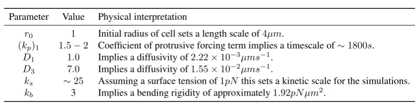
Parameter Value Physical interpretation
r0 1 Initial radius of cell sets a length scale of4µm.
(kp)1 1.5−2 Coefficient of protrusive forcing term implies a timescale of∼1800s. D1 1.0 Implies a diffusivity of2.22×10−3µms−1.
D3 7.0 Implies a diffusivity of1.55×10−2µms−1.
ks ∼25 Assuming a surface tension of1pNthis sets a kinetic scale for the simulations. kb 3 Implies a bending rigidity of approximately1.92pN µm2.
TABLE2. Physically relevant parameter values for simulations on curves.
expansion). As the local maxima corresponding to the activator peak is reduced most at the tip of the peak, where protrusion is largest, this has the effect of increasing the propensity of activator peaks and hence pseudopods to split.
We may proceed to estimate some of the parameter values using available experimental data, which is readily available for dictyostelium cells [2]. The typical radius of cell cross sections is4µmwhich sets the length scale for the computations. The maximum actin polymerisation velocity (which is related to the nondimensional parameter(kp)1) is approximately0.1ms−1, thus the value of(kp)1together with
the maximum density ofa1in the simulations (approx. 30) sets the timescale for the simulations. Typical
values of the surface tension are10pN/µm, assuming a cell height of0.1µmthis sets a kinetic scale for the simulation. The remaining physically relevant parameters may thus be estimated and are given in Table 2. Note that the timescale we refer to in Table 2 corresponds to one unit of computational time. The length of the simulations in Figure 3 is one computational time unit or thirty minutes in actual time and corresponds to roughly 20 pseudopod lifetimes (Each change in direction in Figure 3 represents a pseudopod splitting/decay event), thus the timescale of an individual pseudopod is around ninety seconds.
We note that other choices of the material parameters, specifically weaker surface tension, gives cells with more elongated shapes, larger protrusions and cell bodies which appear less rounded.
4.1.2. Migration in the presence of a chemoattractant. We now include a chemoattractant in the model. We use the stochastic receptor model proposed by Neilson et al. [7] to model the noisy chemotactic signalling. For completeness we state the essential details. At timet ∈ (0, T]they model the cells sensing of the chemotactic signalRtwith an Ornstein-Uhlenbeck stochastic process of the form
(4.4) dRt=θ(µ−Rt) dt+σdWt,
whereWtdenotes the Wiener process, µ(x, t)models the strength of the chemotactic signal, θ(x, t)
the rate of reversion to the meanµandσ(x, t)the variance. The meanµis local and prescribed by the model, while the rate of reversion to the mean and variance are local too as they are chosen such that θ = 1/(1−µ)andσ= cµ1/2(for details see [7,§6.2.2]). To compare with [7,§6.2.5], we model the
signal such that if a chemoattractant is present the meanµvaries from the base signal strength (at the back of the cell) of0.5to0.5 +ρat the front, whereρ >0represents the signal strength. For a given signal directiondsthe position of the rear of the cellxris such thatxr·ds= minΓ(x·ds). We have
also conducted experiments whereµ= exp(−c|x−xc|), wherexcdenotes the location of a static point
source of chemoattractant and observe similar results. We discretise (in space) by assuming the meanµ is constant over each finite element, and henceθandσare also constant on each finite element.
Figure 4 shows the trajectories of the centroids of 5 cells migrating leftwards in a linear chemotactic gradient of varying strength under conserved surface tension evolution (ks = 25, kb= 0,(kp)1 = 1.5).
The results are similar under the other geometric evolution considered (ks= 22, kb= 3,(kp)1= 2) and
[image:9.595.104.523.93.197.2](a) Spider plots of cell centroid trajectories over the interval[0,1.], under conserved surface tension evol-ution, for parameter values see Table 1 and the text.
(b) Spider plots of cell centroid trajectories over the interval[0,1.], under a combination of surface tension and elastic evolution, for parameter values see Table 1 and the text.
FIGURE3. (Online version in colour.) Centroid trajectories of 5 cells migrating in the
absence of a chemoattractant under different geometric evolution laws. In both cases we see motion in a straight line for short times punctuated by sharp changes in direction corresponding to pseudopod splitting/decay.
the absence of a chemoattractant. As the signal strength is increased (at a signal strength of 0.04 around 8%of the base signal) the cells start to exhibit a clear directional preference and successfully navigate up the chemotactic gradient. In Table 3 we report on chemotaxis measures of 100 cells migrating under the 6 different signal strengths shown in Figure 4. We state the average value over the 100 simulations (for each signal strength) of the following quantities all evaluated att= 0.5:
• The chemotactic index (CI), defined as the cosine of the angle between a line connecting the present position of the cell centroid to the starting point and a line directly up the chemotactic gradient [39]. • The persistence length (PL) of the centroid trajectory in thexandydirections. The persistence length
is taken to be the displacement in the chosen direction divided by the total length of the trajectory of the cell centroid [40].
• The squared displacement of the cell centroid from its initial position. • The speed of the cell.
Signal strength CI PL (x) PL (y) 0 N/A 0.4336 (0.2346) 0.4601 (0.2442) 0.02 0.7196 (0.2877) 0.4938 (0.2188) 0.3418 (0.1999) 0.04 0.9423 (0.0742) 0.6968 (0.1177) 0.2005 (0.1163) 0.06 0.9888 (0.0133) 0.8510 (0.0511) 0.1088 (0.0685) 0.08 0.9860 (0.0120) 0.8490 (0.0350) 0.1288 (0.0676) 0.1 0.9898 (0.0141) 0.8489 (0.0272) 0.0987 (0.0734) Signal strength Squared displacement (arb) Speed (arb) Speed (µm/s)
0 37.052 (14.5937) 20.056 (1.9781) 0.0445 0.02 34.430 (13.5045) 19.799 (2.8624) 0.0440 0.04 44.655 (11.9692) 20.077 (2.8633) 0.0446 0.06 66.011 (10.3248) 21.156 (1.9327) 0.0470 0.08 66.491 (6.8996) 21.524 (1.9714) 0.0478 0.1 67.387 (8.8005) 21.435 (2.1560) 0.0476 TABLE 3. Mean and standard deviation (in parentheses) of chemotaxis measures at t= 0.5for 100 cells migrating as in Figure 4.
strength. The (physical) cell speeds are similar to those observed in migrating leukocytes [41, Tab. 1] and Dictyostelium cells [39] (in both cases reported inµm/min).
We now investigate the ability of this model to capture the ability of a cell to respond to a changing chemotactic signal. We use the same stochastic receptor model for the chemotactic signalling but now we change the direction of the signal at various stages in the evolution. Figures 5(a) and 5(b) show snapshots of the cells shaded by activator concentration under the two different geometric evolutions (ks = 25, kb = 0,(kp)1 = 1.5andks = 22, kb = 3,(kp)1= 2) in response to a changing chemotactic
signal. Initially we include only the base signal with noise, i.e., the signal strength is set to zero. At the times in the evolution at which the arrows appear in the figure we change the direction of the signal, with signal strengthρ= 0.1, to the direction indicated by the arrows. We see that under both geometric evolutions the cell successfully responds to the changing signal exhibiting a clear directional preference for movement in the direction of higher chemoattractant concentration. As a final example of response to a changing signal, we consider the case where the signal direction is changed by 180 degrees. The results of such a simulation are shown in Figure 6. We observe the cell successfully responds to the change in signal direction and does so via turning gradually through 180 degrees. This corresponds to so called “hops” (consecutive right/right or left/left splitting of pseudopods) that are an important mechanism for the reorientation of Dictyostelium cells moving in a direction more than 90 degrees off the chemotactic gradient [42, Fig. 4]. Under this model, we have however thusfar not observed the formation ofde novo pseudopods towards the direction of increasing chemoattractant, which are another significant mechanism for major directional corrections [42].
(a)ρ= 0.0 (b)ρ= 0.02 (c)ρ= 0.04
(d)ρ= 0.06 (e) ρ= 0.08 (f)ρ= 0.1
FIGURE 4. (Online version in colour.) Centroid trajectories of 5 cells migrating
left-wards in the presence of a linear chemoattractant gradient under conserved surface tension evolution with varying signal strength (ρ).
LetNo ∈ Ndenote the number of obstacles with centres{mi}i=1No and radii{ri}Ni=1o. For the force
acting on a pointx∈Γ(t)on the cell boundary due to the interaction with obstacleiwe postulate
(4.5) Fo,i= max (0,(ri(1 +)− |mi−x|)) ((mi−x)·(−ν))
fi
|mi−x| −ri
wherefi>0is a material coefficient andε >0is a thickness parameter: the force is zero if the distance
between the cell membrane and the obstacle boundary is bigger thanεri. The force becomes infinite as
this distance approaches zero and then dominates any other forces on the cell membrane, thus preventing intersection of the cell and the obstacle. The external force acting on the cell boundary is given by
(4.6) Fext=
No
X
i=1
Fo,i
For the obstacle particles we postulate a viscous motion law, too, where the reaction forces from the cell boundary−Fi,oand obstacle-obstacle interactions are taken into account. We postulate
(4.7) ωim˙ i=− Z
Γ(t)
Fi,oνdS+ X
j6=i
Fj,i.
Here, theωi >0are positive kinetic coefficients related to the mass of the particle, the first term on the
right hand side modelling the cell-obstacle interaction is
(4.8) Z
Γ(t)
Fi,oνdS= Z
Γ
max (0,(ri(1 +)− |mi−x|)) ((mi−x)·ν)
fi
(a) Chemotactic motion of a cell under con-served surface tension evolution, for para-meter values see Table 1 and text. Cell out-lines shown every.1units of computational time over the interval[0,1.8].
(b) Chemotactic motion of a cell under a com-bination of surface tension and elastic evolution with volume conservation, for parameter values see Table 1 and text. Cell outlines shown every .075units of computational time over the interval [0,1.725].
FIGURE 5. (Online version in colour.) Response to a changing chemotactic signal. Initially there is no signal with arrows indicating the time at which a signal is introduced and the signal direction. Note the two figures are not on the same scale and the cells have the same enclosed volume.
Reaction kinetic parameters
D1 D3 γ r1 r3 s1 s3 b1 b3
10 70 5×10⁴ 2×10⁻² 13×10−3 1×10⁻⁴ 0.2 0.1 5×10⁻³
TABLE 4. Parameter values for numerical experiments of the movement of
three-dimensional cells with the Meinhardt kinetics 4.1.
Parameter Value Physical interpretation
r0 1 Initial radius of cell sets a length scale of1.17µm.
(kp)1 0.5 Coefficient of protrusive forcing term implies a timescale of∼230s. D1 10 Implies a diffusivity of5.95×10−2µm2s−1.
D2 70 Implies a diffusivity of4.17×10−1µm2s−1.
ks ∼25 Assuming a surface tension of10pN/µm, sets kinetic scale.
TABLE5. Physically relevant parameter values for simulation of migration of a cell in
three dimensions.
and theFj,iis the force from particlejexerted on particleifor which we postulate
(4.9) Fj,i= max (0,(1 +)(ri+rj)− |mi−mj|)
fji
|mi−mj| −(ri+rj)
mi−mj
where thefji=fij>0are material coefficients. Note that in the absence of the cell, the initial location
of the obstacles is such that the sum of the forces Fj,i yields zero so that the particles do not move.
Moreover we have the following balance of forces exerted by the cell on the obstacles and forces on the cell membrane due to the obstacles
Z
Γ
Fextν + No X i=1 Z Γ
− Fi,oν
+X
j6=i
Fj,i
= 0.
Figures 7 and 8 show a series of snapshots of cell migration through a field of obstacles, with parameter values as in Table 1 and the two previously considered geometric evolutions. Our numerical experience suggests that under the simple model of cell obstacle interactions we have employed, the increase in computational time, even with a large number of obstacles, from the case of no obstacles is negligible. We include the forcing terms in the evolution law for the cell membrane and the obstacle centres given by (4.6)—(4.9), with parameter values= 0.1, fi =fij= 100for alli, jandωi=ri/100. We observe
that the cell successfully migrates through the field of obstacles maintaining the characteristic shape as it deflects the obstacles. Our numerical experiments suggest that this behaviour is sensitive to the parameter values chosen in the repulsive potential (4.5). In particular, if we set the kinetic coefficient related to the mass of the obstaclesωi c.f., (4.8) to be comparable in magnitude to the kinetic coefficient related to
the mass of the cell (1 by assumption), which means the obstacles inhibit more strongly the protrusion of pseudopods, then pseudopod splitting no longer occurs and the cell exhibits persistent motion in the direction of an obstacle (not reported).
4.1.4. Migration of cells in three space dimensions. We now present results for the motion of three-dimensional cells in the absence of a chemoattractant. We took the unit sphere as the initial steady state and used the reaction kinetic parameter values given in Table 4. We selected a timestep of10−5and used
the adaptive strategy described in the ESM with parametersNH = 0.5, Nh = 0.75, MH = 0.25and Mh= 0.5. We considered an evolution law of the form (2.8) with parametersks= 25, kb = 0,(kp)1 =
(a)t= 0 (b)t= 0.15 (c)t= 0.25
(d)t= 0.375 (e)t= 0.5 (f) t= 0.625
(g)t= 0.75 (h) t= 0.875 (i)t= 1
FIGURE 7. (Online version in colour.) Undirected migration (i.e., migration in the
absence of a chemoattractant) in the presence of obstacles of a cell under conserved surface tension evolution, for parameter values see Table 1 and text.
(a)t= 0 (b)t= 0.15 (c)t= 0.25
(d)t= 0.375 (e)t= 0.5 (f)t= 0.6
(g)t= 0.75 (h)t= 0.875 (i) t= 1
FIGURE 8. (Online version in colour.) Undirected migration in the presence of
We also observe pseudopod splitting as the cell changes direction via biased generation and retraction of existing pseudopods. The simulation is considerably more challenging than the curve case considered previously and the total CPU time of the simulation was just over 27 hours.
(a)t= 0 (b)t= 0.09 (c)t= 0.015
(d)t= 0.025 (e) t= 0.035 (f)t= 0.055
(g)t= 0.075 (h)t= 0.085 (i) t= 0.09
(j)t= 0.095 (k)t= 0.1
FIGURE9. (Online version in colour.) Migration in the absence of a chemoattractant
of a three-dimensional cell under conserved surface tension evolution, for parameter values see Table 4 and text.
5. MODELLING THE PERSISTENT MOTION OF KERATOCYTES
Reaction kinetic parameters Surface evolution parameters D1 D2 γ k1 ks kb (kp)1 (kp)2
0.5 50 10 0.1 2 2 −2 1
TABLE 6. Parameter values for numerical experiments of keratocyte movement with
the RDS (5.1).
if movement of the cell is disrupted the cell rapidly regains its previous shape and speed of movement, usually moving in a new direction.
The observed behaviour of spontaneous polarisation and subsequent development of a steady state stable to perturbations, suggests a Turing type mechanism coupled to a surface evolution law could accur-ately capture the observed dynamics. Shao et al. [22] considered a membrane subject to surface tension, bending rigidity, and forcing with volume conservation. The forcing strength was dependent on the con-centrations of a two component RDS posed in the bulk of the cell. They present computational results, for two-dimensional cells with weak volume conservation (enforced via penalisation), based on a phase field method. Ziebert et al. [6] present a model for keratocyte movement, again based on a phase field method, where they couple the surface evolution to a vector field that seeks to describe the polarisation of the actin network. Studies suggest that branched filamentary actin and actin bundles are concentrated primarily near the cell membrane near areas of protrusion and retraction respectively, while away from the cell surface the actin is in a remodelling phase between that of branched and bundled actin [18, 45, 46]. This suggests a surface model where the pattern formation process occurs on the cell membrane itself may be appropriate. We propose theactivator-depletedsubstrate model [47]:
∂•a1+a1∇Γ(t)·V −D1∆Γa1=γ k1−a1+a21a2
,
∂•a2+a2∇Γ(t)·V −D2∆Γa2=γ k2−a21a2
, onΓ(t), t >0,
a(·,0) =a0(·) onΓ0.
(5.1)
We first present results for curves, with material and RDS parameters given in Table 6. We considered an initially circular cell with radius 1 centred at the origin. The initial condition for the RDS was taken as the linearly stable steady statea0
1=k1+k2, a02 =k2/(a01)2with a symmetry breaking perturbation
of the form max(1×10−4x
1,0) added to the initial condition of thea2 species. The specific form
of the initial condition leads to cells that migrate only along thexaxis (we verified that the choice of other initial conditions only changed the direction of the movement). The hypothesis of Keren et al. is that variability in the actin dynamics is the major factor governing the observed variations in shape and speed. To investigate this hypothesis, we propose that thea1species in the RDS (5.1) corresponds to the
density of retraction promoting actin bundles while thea2species corresponds to the density of protrusion
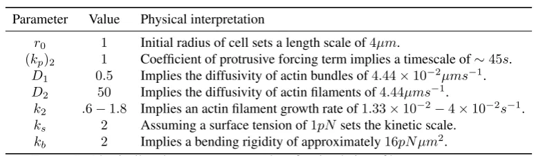
promoting actin filaments, which is similar to the model considered in [22]. We can model variable actin dynamics by changing the constant k2 which can be interpreted as the growth rate of actin filaments.
Increasingk2leads to higher concentrations of a2relative toa1 and thus should lead to faster moving
cells with stronger forcing at the front.
In all the simulations on curves we used an initially equidistributed mesh with 1024 degrees of freedom and a fixed timestep of10−3. The CPU times were on the order of seconds with a typical simulation taking approximately 200 seconds. Figures 10(a) and 10(b) show, for different values ofk2, the initial position
of the cells at time 0 and the cell positions and surface RDS concentrations at time 5 (by which time all the cells have reached a steady state with constant speed and time independent RDS concentrations). We see faster cell speeds and larger aspect ratios for increased values ofk2, similar to the models where
Parameter Value Physical interpretation
r0 1 Initial radius of cell sets a length scale of4µm.
(kp)2 1 Coefficient of protrusive forcing term implies a timescale of∼45s. D1 0.5 Implies the diffusivity of actin bundles of4.44×10−2µms−1. D2 50 Implies the diffusivity of actin filaments of4.44µms−1.
k2 .6−1.8 Implies an actin filament growth rate of1.33×10−2−4×10⁻²s−1. ks 2 Assuming a surface tension of1pNsets the kinetic scale.
kb 2 Implies a bending rigidity of approximately16pN µm2.
TABLE7. Physically relevant parameter values for simulation of keratocyte movement in two-dimensions.
(a) Activator (a1) concentrations
(b) Substrate (a2) concentrations
FIGURE 10. (Online version in colour.) Initial position (att = 0 right hand cell) and persistent keratocyte like migration of cells (at t = 5). The parameterk2 =
0.6,0.8,1.0,1.2,1.4,1.6,1.8reading from right to left for the 7 polarised (left hand) cells (c.f. (5.1)) with the remaining parameters given in Table 6.
We report on the aspect ratioAR= (λ2/λ1)1/2, as considered in [6], where fori= 1,2,λiis as follows
(theλi’s are the eigenvalues of the diagonal2×2variance matrix of the cells centroid):
λi=
1 3
Z
Γ
(xi−xci)3νids,
wherexc
i is the ith coordinate of the cells centroid. We also report on the deviation from reflection
symmetry of the migrating cells as considered in [6]. This is measured by the following quantities (the nonzero components of the skewness tensor of the cells centroid scaled by a constant factor):
η1= 1
4
Z
Γ
(x1−xc1) 4ν
1ds 1/3
(λ1+λ2)−1/2,
η2= 1
2
Z
Γ
(x1−xc1) 2(x
2−xc2) 2ν
1ds 1/3
[image:19.595.121.509.96.209.2](λ1+λ2)−1/2.
[image:19.595.202.438.608.666.2]0 1 2 3 4 5 0
1 2 3 4 5 6
Time
Speed
0 1 2 3 4 5
1 1.5 2 2.5
Time
Aspect ratio
k
2=0.6 k2=0.8 k2=1.0 k2=1.2 k2=1.4 k2=1.6 k2=1.8
FIGURE11. (Online version in colour.) The speed of the cell centroid and aspect ratio both vs. time of the cells shown in Figure 10. We observe a positive relationship between aspect ratio and speed.
0 1 2 3 4 5
0 0.05 0.1 0.15 0.2
Time
η
1
0 1 2 3 4 5
0 0.05 0.1 0.15 0.2 0.25 0.3
Time
η 2
k
2=0.6 k2=0.8 k2=1.0 k2=1.2 k2=1.4 k2=1.6 k2=1.8
FIGURE 12. (Online version in colour.) Asymmetry measures vs. time of the cells
shown in Figure 10. We observe larger deviations from reflection symmetry in the cells travelling at slower speeds. As the cells attain persistent shapes the values converge to a steady state.
studies. In physical units the range of the speed at steady state of the cells shown in Figure 10 is0.178to 0.445µms−1. Both the speed and aspect ratios are similar to those observed in the experimental results reported in [18, Figure 4b]. Figure 12 shows values of the asymmetry measures against time. We see that the cells travelling at slower speed exhibit larger deviations from reflection symmetry. This is in contrast to the results obtained under the model considered in [6, Fig. 4], whereη1does increase as the speed of
the cells decreases butη2is positively correlated with speed. We note that for the first two simulations k2 = 0.6 and0.8,η2 is negatively correlated with speed. As an ellipse satisfies η1 = η2 = 0, it is
reported values oscillate, the values converge to a steady state as the cells travel in a persistent fashion with a fixed shape and a constant speed.
(a) Activator (a1) concentrations
(b) Substrate (a2) concentrations
FIGURE 13. (Online version in colour.) Initial position (att = 0 right hand cell) and persistent keratocyte like migration of cells (at t = 5). The parameterk2 =
0.6,0.7,0.8,0.9,1.0reading from right to left for the 5 polarised (left hand) cells (c.f. (5.1)), for the remaining parameter values see Table 8.
0 2 4 6
0 1 2 3 4 5 6 7 8
Speed
Time
0 2 4 6
12.5 12.55 12.6 12.65 12.7 12.75 12.8 12.85 12.9 12.95 13
Surface Area
Time k
2=0.6 k2=0.7 k2=0.8 k2=0.9 k2=1.0
FIGURE14. (Online version in colour.) The speed of the cell centroid and cell surface
area both vs. time of the cells shown in Figure 13. We observe a positive relationship between surface area and speed.
Reaction kinetic parameters Surface evolution parameters Adaptive strategy parameters D1 D2 γ k1 ks kb (kp)1 (kp)2 NH Nh MH Mh
1 100 20 0.1 1 1 −0.7 .35 .5 1 .25 .5 TABLE8. Parameter values for numerical experiments of three-dimensional keratocyte
movement with the RDS (5.1) and surface evolution law 2.8.
Parameter Value Physical interpretation
r0 1 Initial radius of cell sets a length scale of1.17µm.
(kp)2 .35 Coefficient of protrusive forcing term implies a timescale of∼4s. D1 1.0 Implies the diffusivity of actin bundles of0.342µm2s−1.
D2 100 Implies the diffusivity of actin filaments of34.2µm2s−1. k2 .6−1.0 Implies an actin filament growth rate of0.15×10−1−0.25s−1. ks 1 Assuming a surface tension of10pN µm−1, sets the kinetic scale. kb 1 Implies a bending rigidity of approximately13.69pN µm.
TABLE9. Physically relevant parameter values for simulation of keratocyte movement
in three-dimensions.
timestep of10−4 and remaining parameter values for both the surface evolution and adaptive strategy as given in Table 8. The CPU times were on the order of minutes with a typical simulation taking approximately 2000 seconds. Proceeding as in §4, we give physical interpretations of the parameter values for curves and surfaces in Tables 7 and 9 respectively. Figures 13(a) and 13(b) show a similar experiment to the one carried out for curves now on surfaces, specifically we report for different values of k2, the initial position of the cells at time 0 and the cell positions and surface RDS concentrations at time
5 (by which time all the cells have reached a steady state with constant speed and time independent RDS concentrations). The gross behaviour is the same as the curve case, in that as the parameterk2is increased
from0.6to1the cells move faster at steady state and appear more elongated. Figure 14 shows plots of the speed of the cell centroids and the surface area of the cells both against time. We plot the surface area as it is proportional to the two, roughly equal, aspect ratios in the(x, y)and(x, z)directions. We observe the same positive relationship as in the curve case with both surface area and speed converging to steady states. We have also verified that the aspect ratios converge to steady states with the aspect ratio in the(y, z)direction approaching 1. Note for larger values ofk2the cells developed a self intersection
which is inadmissible under our modelling as it would correspond to a change in topology in the physical setting. Scenarios where one wishes to consider topological change, or respectively methods that avoid topological change, are a subject of our current research.
6. CONCLUSION
In this work we have presented a computational framework for the modelling of cell motility. We pro-pose a simple and consistent means of coupling cell movement with gradient sensing, polarisation using surface PDEs and external forces. Our methods can be generalised to the modelling of more complex phenomena such as adhesion and crawling on a substrate or cell-cell interactions and we illustrate one such generalisation with a concrete example of migration in the presence of obstacles.
both the continuous and discrete problems are posed in one dimension less than the underlying spatial di-mension, which in the case of the discrete problem typically means fewer degrees of freedom are needed than would be the case for embedded methods [10, 13, 14, 15, 16]. On curves, our experience is that the method maintains a mesh suitable for computation without the use of remeshing or adaptive mesh refinement. For the simulations of cell migration in three-dimensions we occasionally observed deterior-ation in the mesh quality, even with the redistribution of the vertices implicit in our numerical scheme, necessitating spatial adaptivity. An area of our ongoing research is the investigation of numerical methods robust to large deformations in the cell surface.
We consider a pseudopod centred model for chemotaxis similar in form to that considered in [37]. Unlike compass models [39], which are reasonable for cells with flexible polarity where a large gradient may induce pseudopods at any position on the cell membrane, pseudopod centred models [17] are suitable for strongly polarised cells where pseudopods are generated preferentially at the front with directional bias, due to a chemotactic gradient, restricted primarily to small changes in direction [42]. The major contributions and imports of our study are the inclusion of bending rigidity, the inclusion of external forces, the observation that the gross behaviour, of pseudopod splitting, observed in [37] for2dcells persists in3dsimulations and that the model remains qualitatively unchanged when one considers a two component RDS, with a spatially constant global inhibitor, rather than a three component RDS with a biologically implausible non-local term. Our computational method based on surface finite elements extends the method in [16] and is an alternative to the level set method considered in [7, 37]. The simulations illustrate that the model is capable of reproducing aspects of pseudopod-driven cell migration, described in [17], in both two and three space dimensions. We report on many widely used chemotaxis measures and observe values similar to experimental observations. We also note that the simulations exhibit a dilution effect at the tip of a pseudopod where the local maxima corresponding to an activator peak is reduced. This suggests experimental investigation of the relative importance of mechanical effects of membrane protrusion on the distribution of cell resident proteins is warranted.
We also investigated a model for the motion of fish keratocytes. The model appears to reproduce some experimental observations of the shapes of motile keratocyte cells and the experimental observation of the correlation between cell shape and speed [18]. The computational model in [18] reproduces the velocity-aspect ratio relationship. However, unlike our model, both polarisation and cell shapes are not explicitly modelled, with a parabolic actin profile at the leading edge assumed and the shape of the cell rear neglected. Studies [6] and [22] propose models where polarisation is modelled by equations in the bulk of the cell which are coupled to an evolution law for the cell surface. The import of our study is to show that a surface RDS coupled to a surface evolution law gives qualitatively similar results. A further contribution is the use of surface finite elements rather than the phase field method considered in [6] and [22]. This allows simulation of3dkeratocyte migration which studies [6] and [22] both note is computationally expensive with the phase field methodology. We do observe minor differences from [6], for example in the measures of deviation from reflection symmetry.
Our numerical experience suggests that some aspects of cell migration and chemotaxis can be cap-tured by the Schnakenberg RDS (5.1). This RDS is considerably simpler from a mathematical analysis viewpoint than say the Meinhardt model (4.1). One can show that the model is well posed on evolving (planar) domains [48], which is an open question even on fixed domains for the Meinhardt model. As the two components are out of phase the model lends itself naturally to the case of a species that promotes protrusion (e.g., actin) and another that promotes retraction (e.g., myosin).
ACKNOWLEDGMENTS
This research has been supported by the UK Engineering and Physical Sciences Research Council (EPSRC), Grant EP/G010404.
REFERENCES
[1] D. Bray.Cell movements: from molecules to motility. Routledge, 2001.
[2] A. Mogilner. Mathematics of cell motility: have we got its number? Journal of mathematical biology, 58(1):105–134, 2009.
[3] A. Jilkine and L. Edelstein-Keshet. A comparison of mathematical models for polarization of single eukaryotic cells in response to guided cues.PLoS Computational Biology, 7(4), 2011.
[4] J.C. Del Alamo, R. Meili, B. Alonso-Latorre, J. Rodr´ıguez-Rodr´ıguez, A. Aliseda, R.A. Firtel, and J.C. Lasheras. Spatio-temporal analysis of eukaryotic cell motility by improved force cytometry. Proceedings of the National Academy of Sciences, 104(33):13343, 2007.
[5] M.L. Lombardi, D.A. Knecht, M. Dembo, and J. Lee. Traction force microscopy in dictyostelium reveals distinct roles for myosin ii motor and actin-crosslinking activity in polarized cell movement. Journal of Cell Science, 120(9):1624–1634, 2007.
[6] F. Ziebert, S. Swaminathan, and I.S. Aranson. Model for self-polarization and motility of keratocyte fragments.Journal of The Royal Society Interface, 2011.
[7] M.P. Neilson, J. Mackenzie, S. Webb, and R.H. Insall. Modelling cell movement and chemotaxis pseudopod based feedback.SIAM Journal on Scientific Computing, 33(3), 2011.
[8] JM Oliver, JR King, KJ McKinlay, PD Brown, DM Grant, CA Scotchford, and JV Wood. Thin-film theories for two-phase reactive flow models of active cell motion.Mathematical Medicine and Biology, 22(1):53–98, 2005.
[9] W. Alt and M. Dembo. Cytoplasm dynamics and cell motion: two-phase flow models.Mathematical biosciences, 156(1-2):207–228, 1999.
[10] G. Dziuk and C.M. Elliott. Finite elements on evolving surfaces.IMA journal of numerical analysis, 27(2):262, 2007.
[11] J.W. Barrett, H. Garcke, and R. N¨urnberg. Parametric approximation of Willmore flow and related geometric evolution equations.SIAM Journal on Scientific Computing, 31:225, 2008.
[12] L. Yang, J. Effler, B. Kutscher, S. Sullivan, D. Robinson, and P. Iglesias. Modeling cellular deform-ations using the level set formalism.BMC systems biology, 2(1):68, 2008.
[13] C. Landsberg and A. Voigt. A multigrid finite element method for reaction-diffusion systems on surfaces.Computing and Visualization in Science, 13(4):177–185, 2010.
[14] G. Dziuk and C.M. Elliott. Eulerian finite element method for parabolic pdes on implicit surfaces. Interfaces and Free Boundaries, 10(119-138):464, 2008.
[15] R.I. Saye and J.A. Sethian. The voronoi implicit interface method for computing multiphase physics. Proceedings of the National Academy of Sciences, 108(49):19498–19503, 2011.
[16] M.P. Neilson, J.A. Mackenzie, S.D. Webb, and R.H. Insall. Use of the parameterised finite element method to robustly and efficiently evolve the edge of a moving cell.Integr. Biol., 2010.
[17] R.H. Insall. Understanding eukaryotic chemotaxis: a pseudopod-centred view. Nature Reviews Molecular Cell Biology, 11(6):453–458, 2010.
[18] K. Keren, Z. Pincus, G.M. Allen, E.L. Barnhart, G. Marriott, A. Mogilner, and J.A. Theriot. Mech-anism of shape determination in motile cells.Nature, 453(7194):475–480, 2008.
[19] J.D. Murray.Mathematical biology. Springer Verlag, 2003.
[21] R. Barreira, C.M. Elliott, and A. Madzvamuse. The surface finite element method for pattern form-ation on evolving biological surfaces. Journal of Mathematical Biology, pages 1–25, 2011. ISSN 0303-6812.
[22] D. Shao, W.J. Rappel, and H. Levine. Computational model for cell morphodynamics. Physical review letters, 105(10):108104, 2010.
[23] David Traynor and Robert R. Kay. Possible roles of the endocytic cycle in cell motility. Journal of Cell Science, 120(14):2318–2327, 2007. doi: 10.1242/jcs.007732. URL http://jcs. biologists.org/content/120/14/2318.abstract.
[24] K. Larripa and A. Mogilner. Transport of a 1d viscoelastic actin-myosin strip of gel as a model of a crawling cell. Physica A: Statistical Mechanics and its Applications, 372(1):113–123, 2006. [25] K. Deckelnick, G. Dziuk, and C.M. Elliott. Computation of geometric partial differential equations
and mean curvature flow. Acta Numerica, 14:139–232, 2005. ISSN 0962-4929.
[26] W. Helfrich. Elastic properties of lipid bilayers: theory and possible experiments. Z. Naturforsch, 28(11):693–703, 1973.
[27] T.J. Willmore.Riemannian geometry. Oxford University Press, USA, 1997.
[28] G. Dziuk. An algorithm for evolutionary surfaces. Numerische Mathematik, 58(1):603–611, 1990. [29] G. Dziuk and C.M. Elliott. L2-estimates for the evolving surface finite element method.Math Comp
(to appear), 2012.
[30] C.M. Elliott and B. Stinner. Modeling and computation of two phase geometric biomembranes using surface finite elements. Journal of Computational Physics, 229(18):6585–6612, 2010.
[31] C.M. Elliott and B. Stinner. Computation of two-phase biomembranes with phase dependent mater-ial parameters using surface finite elements. CiCP (to appear), 2012.
[32] CJ Heine. Isoparametric finite element approximation of curvature on hypersurfaces. Preprint. [33] G. Dziuk. Computational parametric Willmore flow.Numerische Mathematik, 111(1):55–80, 2008. [34] A. Schmidt and K.G. Siebert.Design of adaptive finite element software: The finite element toolbox
ALBERTA. Springer Verlag, 2005.
[35] Timothy A. Davis. Algorithm 832: Umfpack v4.3—an unsymmetric-pattern multifrontal method. ACM Trans. Math. Softw., 30:196–199, June 2004. ISSN 0098-3500. doi: http://doi.acm.org/10. 1145/992200.992206. URLhttp://doi.acm.org/10.1145/992200.992206.
[36] H. Meinhardt. Orientation of chemotactic cells and growth cones: models and mechanisms.Journal of Cell Science, 112(17):2867, 1999.
[37] M.P. Neilson, D.M. Veltman, P.J.M. van Haastert, S.D. Webb, J.A. Mackenzie, and R.H. Insall. Chemotaxis: A feedback-based computational model robustly predicts multiple aspects of real cell behaviour. PLoS biology, 9(5):e1000618, 2011.
[38] D.P. Amarasinghe, A. Aylwin, P. Madhavan, and C. Pettitt. Biomembranes report. MASDOC, RSG, 2011.
[39] I. Hecht, M.L. Skoge, P.G. Charest, E. Ben-Jacob, R.A. Firtel, W.F. Loomis, H. Levine, and W.J. Rappel. Activated membrane patches guide chemotactic cell motility.PLoS Computational Biology, 7(6):e1002044, 2011.
[40] S.Y. Cheng, S. Heilman, M. Wasserman, S. Archer, M.L. Shuler, and M. Wu. A hydrogel-based microfluidic device for the studies of directed cell migration.Lab Chip, 7(6):763–769, 2007. [41] WS Ramsey. Analysis of individual leucocyte behavior during chemotaxis. Experimental cell
research, 70(1):129–139, 1972.
[42] L. Bosgraaf and P.J.M. Van Haastert. Navigation of chemotactic cells by parallel signaling to pseudopod persistence and orientation. PloS one, 4(8):e6842, 2009.
[43] I. Hecht, H. Levine, W.J. Rappel, and E. Ben-Jacob. “self-assisted” amoeboid navigation in complex environments. PloS one, 6(8):e21955, 2011.
[45] L. Bosgraaf, P.J.M. van Haastert, and T. Bretschneider. Analysis of cell movement by simultan-eous quantification of local membrane displacement and fluorescent intensities using quimp2.Cell motility and the cytoskeleton, 66(3):156–165, 2009.
[46] T.D. Pollard and G.G. Borisy. Cellular motility driven by assembly and disassembly of actin fila-ments.Cell, 112(4):453–465, 2003.
[47] R. Lefever and I. Prigogine. Symmetry-breaking instabilities in dissipative systems II. J. chem. Phys, 48:1695–1700, 1968.
[48] Chandrasekhar Venkataraman, Omar Lakkis, and Anotida Madzvamuse. Global existence for semi-linear reaction–diffusion systems on evolving domains. Journal of Mathematical Biology, 64:41– 67, 2012. ISSN 0303-6812. URLhttp://dx.doi.org/10.1007/s00285-011-0404-x.