http://go.warwick.ac.uk/lib-publications
Original citation:
Caudron, Quentin, Donnelly, Simon R., Brand, Samuel P. C. and Timofeeva, Yulia.
(2012) Computational convergence of the path integral for real dendritic morphologies.
The Journal of Mathematical Neuroscience, Volume 2 (Number 1). ISSN 2190-8567
Permanent WRAP url:
http://wrap.warwick.ac.uk/54527
Copyright and reuse:
The Warwick Research Archive Portal (WRAP) makes this work of researchers of the
University of Warwick available open access under the following conditions.
This article is made available under the Creative Commons Attribution 2.0 Generic (CC
BY 2.0) license and may be reused according to the conditions of the license. For more
details see:
http://creativecommons.org/licenses/by/2.0/
A note on versions:
The version presented in WRAP is the published version, or, version of record, and may
be cited as it appears here.
DOI10.1186/2190-8567-2-11
R E S E A R C H Open Access
Computational Convergence of the Path Integral
for Real Dendritic Morphologies
Quentin Caudron·Simon R. Donnelly·Samuel P.C. Brand·Yulia Timofeeva
Received: 19 June 2012 / Accepted: 11 September 2012 / Published online: 22 November 2012 © 2012 Q. Caudron et al.; licensee Springer. This is an Open Access article distributed under the terms of the Creative Commons Attribution License (http://creativecommons.org/licenses/by/2.0), which permits unrestricted use, distribution, and reproduction in any medium, provided the original work is properly cited.
Abstract Neurons are characterised by a morphological structure unique amongst biological cells, the core of which is the dendritic tree. The vast number of dendritic geometries, combined with heterogeneous properties of the cell membrane, continue to challenge scientists in predicting neuronal input-output relationships, even in the case of sub-threshold dendritic currents. The Green’s function obtained for a given dendritic geometry provides this functional relationship for passive or quasi-active dendrites and can be constructed by a sum-over-trips approach based on a path in-tegral formalism. In this paper, we introduce a number of efficient algorithms for realisation of the sum-over-trips framework and investigate the convergence of these algorithms on different dendritic geometries. We demonstrate that the convergence of the trip sampling methods strongly depends on dendritic morphology as well as the biophysical properties of the cell membrane. For real morphologies, the number of trips to guarantee a small convergence error might become very large and strongly affect computational efficiency. As an alternative, we introduce a highly-efficient ma-trix method which can be applied to arbitrary branching structures.
Keywords Dendrites·Path integral·Sum-over-trips·Morphology·Dendritic computation
Q. Caudron (
)·S.P.C. Brand·Y. TimofeevaCentre for Complexity Science, University of Warwick, Coventry, CV4 7AL, UK e-mail:[email protected]
Q. Caudron·Y. Timofeeva
Department of Computer Science, University of Warwick, Coventry, CV4 7AL, UK
S.R. Donnelly
Doctoral Training Centre in Neuroinformatics and Computational Neuroscience, University of Edinburgh, Edinburgh, EH8 9AB, UK
S.P.C. Brand
1 Introduction
Discovered more than a century ago by Santiago Ramón y Cajal [1], dendrites form the vast majority of the surface area of a neuron, with the dendritic trees of some mo-toneurons representing up to 97% of total neuronal surface area and 75% of the total neuronal volume [2]. These complex branching structures are responsible for trans-ferring electrical activity between synapses and the soma. As technology evolved, interest in dendrites began to gather momentum, with the invention of sharp mi-cropipette electrodes in the early 1950s allowing intracellular recordings to be made. It was the breakthrough work of Wilfrid Rall [3] on the application of cable theory to dendritic modelling that provided significant insight into the role of dendrites in processing synaptic inputs, the historical perspective of which is summarised in a book by Segev, Rinzel and Shepherd [4]. Recent experimental and theoretical studies reinforce the fact that dendritic morphology and membrane properties play an impor-tant role in dendritic integration [5,6]. We refer the reader to the bookDendrites[7], devoted exclusively to these formations and revealing their biological complexity at different scales.
It has also been known for some time that nonlinear voltage-gated ion channels are present in the dendrites of various types of neurons [8], and many recent dendritic models are constructed by combining the linear (passive) properties of dendrites to-gether with nonlinear (active) dynamics of membrane channels. Although the nonlin-ear properties of ion channels contribute considerably to neuronal input-output rela-tions, it is important to recognise that the passive properties of dendritic membranes provide the fundamental core for signal filtration and integration, and thus remain an essential component in understanding electrical signalling in dendrites [9].
dendritic geometry as a convergent infinite series solution. Cao and Abbott [21] pre-sented an algorithm for a computational realisation of the sum-over-trips approach, based on the division of trips into four classes. They applied this algorithm to a num-ber of sample dendritic trees, the largest of which had 22 branches, in contrast to real dendritic geometries, which might have more than 400 terminals alone [22], with a large variation in branch length. This complexity in neuronal morphologies across different types of neurons is expected to affect the convergence of computational im-plementations of the sum-over-trips framework.
In this paper, we introduce and investigate a number of efficient algorithms for calculating the Green’s function on dendritic trees using the sum-over-trips formal-ism. In Sect.2, we review the theoretical framework and the four-classes algorithm of Cao and Abbott [21], and introduce alternative algorithms for the sum-over-trips method in Sect.3. We begin with a modification on the four-classes algorithm aimed at improving its time complexity by developing a formal grammar to derive the trips. Then, a length-priority ordering of the trips using Eppstein’s algorithm [23] for find-ing thekshortest trips on a graph is proposed. We also derive a stochastic approach for sampling trips on the tree based on a Monte-Carlo approach. Finally, a highly-efficient deterministic method for discretised tree structures is described. We assess the convergence of the introduced algorithms on different dendritic geometries in Sect.4, where we also compare the delay and attenuation of voltage spread on four reconstructed dendritic morphologies. Finally, in Sect.5, we provide a discussion of our results, as well as possible extensions of this work.
2 The Sum-over-trips Framework
We consider a dendritic branching structure with the dynamics of the membrane volt-age on a finite branchidescribed by the passive cable equation. An external current
Ij(t )is injected at a locationy on branchj. The transmembrane voltage across the
dendritic tree is then described by the following set of equations:
π aiC
∂Vi
∂t = π ai2
4Ra
∂2Vi
∂x2 − π ai
R Vi, 0≤x≤Li, i=j (1)
π ajC
∂Vj
∂t = π aj2
4Ra
∂2Vj
∂x2 − π aj
R Vj+δ(x−y)Ij(t ), 0≤x≤Lj. (2)
Here,aiis the diameter of branchi(measured in µm),Rais the specific cytoplasmic
resistivity (incm),Cis the specific membrane capacitance (in µF cm−2), andRis the resistance across one unit area of passive membrane (incm2). Introducing the electrotonic space constantλi=
√
aiR/(4Ra), the membrane time constantτ =RC
and the diffusion coefficientDi=λ2i/τ, Eqs. (1) and (2) can be rewritten as
∂Vi
∂t =Di ∂2Vi
∂x2 − Vi
τ , 0≤x≤Li, i=j, (3) ∂Vj
∂t =Dj ∂2Vj
∂x2 − Vj
τ +
1
π ajC
In addition to these equations, the appropriate boundary conditions must be specified at all branching nodes and terminals: continuity of the potential across a node and Kirchoff’s law of conservation of current. Continuity of the potential requires that, for all pairs of branchesmandnattached to a node,
Vm(Lm, t )=Vn(0, t ),
where the distal end of branchmis connected to the proximal end of branchn. Con-servation of current for the same node imposes
m
1
rm
∂Vm
∂x
x=Lm
=
n
1
rn
∂Vn
∂x
x=0 ,
wherern=4Ra/(π an2)is the axial resistance on branchn(incm−1), and each sum
is over all branches connected to this node either with their distal or proximal ends. At individual terminals, we can either impose a closed-end boundary condition,
∂Vk
∂x
x=Lk
=0,
or an open-end boundary condition,
Vk(Lk, t )=0,
wherex=Lkis a terminal on branchk.
When the injected current has the form of a delta pulse, that is,Ij(t )=δ(t ), the
solution to Eqs. (3) and (4) is the Green’s functionGij(x, y, t )which can be found
as
Gij(x, y, t )=
1
π ajC
trips
AtripG∞(Ltrip, t ), (5)
where the sum is over all trips (more formally, graph-theoretic walks), starting at
x and finishing aty, and describes the time-course of the membrane voltage at the locationxon branchiin response to the injected current at the locationyon branch
j, whereican be taken to equalj if desired. The functionG∞takes the form
G∞(Ltrip, t )=
1
4π t Dj
e−(Ltrip)2τ /(4t )e−t /τ, (6)
whereLtrip=Ltrip(x/λi, y/λj) is the length of a trip along the tree that starts at
pointx/λi on branchiand ends at pointy/λj on branchj. Note that the length of
each branch needs to be scaled by its own electrotonic space constant beforeLtripis
calculated for Eq. (6). A constructed trip is allowed to reflect on or pass through any node on the tree an arbitrary number of times. The coefficientsAtripdepend on the
constructed trip and are determined according to the following rules [20]:
• For every node at which the trip passes from branchmto branchkwherem=k,
Atripis multiplied by a factor 2pk.
• For every node at which the trip reflects along on a node back onto the same branch
n,Atripis multiplied by a factor 2pn−1.
• For every terminal,Atripis multiplied by+1 for the closed-end boundary condition
or by−1 for the open-end boundary condition.
When the electrical properties of the cell membrane are identical for all branches, the factorspk are defined as
pk=
ak3/2
ma
3/2
m
, (7)
where the sum is over all branchesmconnected to the node. When the parametersR
andRavary from branch to branch, the expression (7) must be modified:
pk=
(λkrk)−1
m(λmrm)−1
. (8)
However, note that the sum-over-trips method for constructing the Green’s function in the time domain only works for uniform characteristic time constantτ across the entirety of the dendritic tree. The generalisation of this framework to support a quasi-active membrane, instead of a passive membrane, releases this restriction and dif-ferent cell membrane properties can be chosen on each branch [24]. However, this means that the construction of the Green’s function as an infinite series solution can only be performed in the Laplace domain.
Knowing the Green’s function for a given dendritic structure allows one to find the voltage response along the entire tree. By finding Gij(x, y, t ) for the ordered
pair(x, y), the Green’s functionGj i(y, x, t )can be found using a simple reciprocity
identity:
Gj i(y, x, t )=
Djrj
Diri
Gij(x, y, t ). (9)
The voltage response can then be found for an arbitrary number of different discrete inputs as a sum of convolution integrals:
Vi(x, t )=
j
t
0
Gij(x, xj, t−s)Ij(s)ds, (10)
wherexjis a location of a stimulusIj(t )on branchj.
The Green’s function calculated by Eq. (5) for any branching structure with finite length branches includes an infinite number of terms. It is possible to show that this infinite series solution converges faster than e−k, for sufficiently-highk, the number
of nodes visited by the trip. We demonstrate this in the Appendix for an arbitrary tree with nodes of degreed=3 or less. This generalises Abbott’s convergence analysis [25], where it was shown that, for an infinite binary tree, the sum of coefficientsAtrip
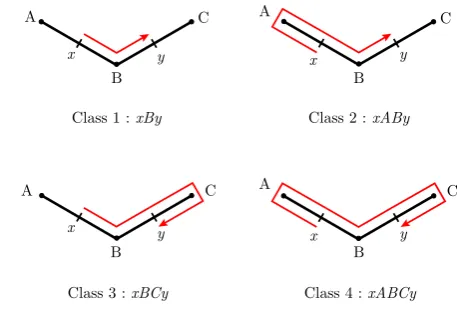
Fig. 1 Four classes of trips between two points.Class 1is the most direct trip, leavingxin the direction ofyand not going pastybefore finishing (xBy). Class 2leavesxin the other direction, but finishes when it meetsy(xABy).Class 3moves fromxtowardsy, but goes past
yand changes direction immediately after passing it before finishing (xBCy). Class 4trips move fromxfirst away from pointyand passy
before reflecting on the next node and finishing (xABCy)
2.1 Four-Classes Algorithm
Cao and Abbott [21] introduced an algorithm for constructing the Green’s function using the sum-over-trips method. Their algorithm is based on finding the shortest trips between any two points of measurementx and current injectiony on a tree. Starting from the most direct, shortest trip fromx toy, passing through the mini-mum number of nodes, four classes of trips are defined by allowing a trip to leave the pointx in either direction and approach y from either direction along their re-spective branches. These initial trips, therefore, form the first and shortest trips in their respective classes; longer trips are generated incrementally from these. New ad-ditional trips can pass the pointsx andy any number of times and are allowed to change direction at any node. We will refer to this method as the four-classes algo-rithm.
Figure1shows a model branching structure with two pointsxandy, and the four shortest classes of trips between them. Trips are represented as sequences of node identifiers, beginning and ending withxandy respectively. For example, we denote a trip fromxtoy via nodesA,BandCby its full description,xABCy.
From these main trips, the four-classes algorithm generates allx →y trips by inserting what are described as “excursions” into the trips. IfAandB are adjacent nodes in a tree, then an excursion could be added to the tripxByto generate the trip
xBABy, representing a reflection on nodeB towardsA, reflecting at the terminal
[image:7.439.158.387.51.211.2]3 Algorithmic Realisations
Here, we suggest possible modifications to the four-classes algorithm of Cao and Abbott [21] as well as introduce novel alternative algorithms for the sum-over-trips formalism.
3.1 Formal Language Theory Approach
The four-classes algorithm generates duplicate trips [21], which must then be re-moved by a binary search through the list of existing trips for every new trip gener-ated, which takesO(klogk)time overall, wherekis the number of trips constructed. There are two different mechanisms by which duplicate trips are generated, and both mechanisms can be eliminated by applying simple restrictions to the choice of excur-sions applicable to a trip. As an example of the first, for the tree in Fig.1, it is possible to generate the tripxBABCByin two different ways from the shortest Class 1 trip,
xBy:
xBy
Excursion
B→BAB
−−−−−→xBABy
Excursion
B→BCB
−−−−−→xBABCBy,
xBy
Excursion
B→BCB
−−−−−→xBCBy
Excursion
B→BAB
−−−−−→xBABCBy.
Due to the fact that the excursion may be added at any step in the trip (at the first or secondB), the same trip may be generated multiple times. If we insist that excursions cannot be added at any step that precedes the excursion most recently added to the trip, this can be prevented. In the theory of context-free grammars, this is equivalent to requiring a leftmost derivation. We can represent this using a symbol to separate the mutable and immutable parts of the trip:
x|By
Excursion
B→B|AB
−−−−−−→xB|ABy
Excursion
B→B|CB
−−−−−−→xBAB|CBy,
x|By
Excursion
B→B|CB
−−−−−−→xB|CBy−−−−−−→ xBABCBy.
The second mechanism by which duplicate trips are produced is the addition of excursions along the same branch, starting from either end. In the structure in Fig.1, we have bothA→A|BAandB→B|AB. Hence, in spite of the leftmost derivation rule, we can generatexABAByin two different ways (brackets added for clarity):
x|ABy→x(A|BA)By,
x|ABy→xA(B|AB)y.
This problem can be avoided by assigning each branch a direction. If the branchAB
of excursions that allow the algorithm to generate trips including it. The allocation of direction to each branch can be performed before the process of generating trips and may coincide with finding the four main classes of trips. These modifications require that the graph be acyclic, since “away from a point” is not generally definable on a graph with cycles. There do exist cyclic graphs for which an unambiguous grammar can generate the language ofx→y trips, but these are not relevant to the study of single dendritic trees.
The two presented modifications of the four-classes algorithm are sufficient to prevent the generation of any duplicate trips, without any trips being missed. To-gether, they provide an unambiguous context-free grammar generating the language ofx→ytrips.
3.2 Length-Priority Method
Since the coefficientsAtripdecay at most with e−Ltrip (although the number of trips
increases with eLtrip), the dominating term in the Green’s function (5) is the exponen-tial decay e−L2trip inG
∞. The four-classes algorithm [21] does not generate trips in monotonic order in length, since trips are constructed by adding the same excursion to all four classes of trips. If, for example, a Class 2 trip is significantly longer than its Class 1 counterpart, due tox being along a long edge but close to a node, then a longer Class 2 trip will be generated before a potentially shorter Class 1 trip having an additional excursion on a shorter branch. In general, trips are likely to be disordered in length if the branches upon whichx or y reside are substantially longer than at least one other branch on the tree, or ifxoryare much closer to one of their adjacent nodes than to the other.
Here, we propose to realise the sum-over-trips framework by a length-priority method. In this implementation, trips are generated and the corresponding terms
AtripG∞(Ltrip, t )are added to the infinite series solution (5) in monotonic order in
lengthLtrip. This is achieved by incorporating Eppstein’s algorithm [23] for finding
thekshortest trips on a graph inO(m+nlogn+k)time, withnbeing the number of nodes andmthe number of edges on the branching structure.
Both the four-classes algorithm and the improvements described in the language-theoretic approach rely on storing trips explicitly as sequences of nodes. This con-sumesO(kn)space and time forktrips withnnodes but allows on-the-fly calculation of coefficientsAtrip. This is contrary to Eppstein’s algorithm [23], which stores trips
3.3 Monte-Carlo Method
The path integral formulation of the solution to the cable equation introduced by Ab-bott et al. [20] is derived via consideration of a Feynman–Kac representation of the solution in terms of random walkers on the dendritic geometry. Hence, it is natural to consider Monte-Carlo approaches to evaluating this path integral. Instead of a length-ordered series solution as provided by the length-priority approach, the Green’s func-tion (5) can be constructed using a stochastic algorithm. The aim of this approach is to sample from tripsx→y in such a way that the probabilistically more likely samples coincide with the trips that contribute most to the series solution (5).
To motivate this Monte-Carlo approach, let us consider a linear diffusion equation along an infinite one-dimensional cable,
∂G ∂t =D
∂2G
∂x2, t∈ [0, T], (11)
satisfying the initial conditionG(x,0)=δ(x−y). Analogously, a diffusion process for the state variableXt can be defined by the stochastic equation
dXt=
√
2DdWt, (12)
with the Wiener processWt and the initial condition X0=y. It is well known that
Eq. (11) is the Kolmogorov equation of the diffusion process (12), that is, the time evolution equation of the probability density for the state of the diffusion (12). On the one hand, solution of (11) via classical numerical or analytical methodology in-forms the probability density ofXt; on the other hand, repeated sampling from (12)
converges upon the solutionG(x, t )of (11). This method of sampling from random walks can also be applied for arbitrary geometries by setting the appropriate boundary conditions at the branching nodes and terminals. KnowingGij(x, y, t )on a branching
structure, we can easily find a solution of the cable equation on this geometry using the relation
Gij(x, y, t )=Gij(x, y, t )e−t /τ.
Because the path integral form of the solution is equivalent to the expectation of a function on random walks upon the branching points of the dendritic tree, reduction of the random walk problem from the complete continuous space geometry of the neuron to the discrete topology of the branching points of the neuron gives a con-siderable efficiency saving to a Monte-Carlo solver. We introduce a parameterkmax,
the maximum number of discrete hops on nodes for which we wish to calculate the expectation. The maximum number is based upon the effective maximum range of diffusion during the interval[0, t]. Then, we generate a realisation of a random walk on the nodes,
ω=(ω1, ω2, . . . , ωkmax), (13)
where each ωk is a label identifying a particular node. For tripsx→y we select
equal probability. By indexing a branch between two nodes,ωk−1andωk, as thekth
branch, subsequent steps are performed with the transition probability
P (ωk|ωk−1)=pk, 2≤k≤kmax, (14)
wherepk is given by (7). This connects the Monte-Carlo method to the earlier
dis-cussed path enumeration methods. Here, we introduce two auxiliary functions,φand
˜
a, of subwalks ofω. The first is a function indicating whether a subwalk ofksteps on a realisationωis a valid trip, and is defined by
φ (y, k, t, ω)=
G∞(L(y, k, ω), t ), ifωk−1andωkare the nodes adjacent toy,
0, otherwise,
wherekis the number of hops on nodes in the subwalk andL(y, k, ω)is the length of the subwalk. The other auxiliary functiona˜is defined as
˜
a(k, ω)= ⎧ ⎪ ⎪ ⎨ ⎪ ⎪ ⎩
1, ifk=1,2,
2, ifωk−2=ωk,
(2pk−1)/pk, ifωk−2=ωk,
1, if at a closed terminal (this takes priority).
The relevant function on paths can be defined as a composite of the auxiliary func-tions described above:
˜
A(y, ω, t )=
kmax
k=1
2φ (y, k, t, ω) k
i=1 ˜ a(i, ω)
.
The expectation ofA˜ with respect to the random walk (14) is equivalent to solving for the path integral, up to some value ofkmaxat timet:
EP
˜
A(y, ω, t )=
ω
P (ω)A(y, ω, t )˜
=
ω kmax
k=1
2P (ω)φ (y, k, ω) k
i=1 ˜ a(i, ω)
=
ω: x→y
atk kmax
k=1
2P (ω)G∞L(y, k, ω), t k
i=1 ˜ a(i, ω)
=
trips
x→y
AtripG∞(Ltrip, t ),
3.4 Matrix Method
An alternative method of constructing the sum-over-trips series solution is by group-ing trips by their lengths:
trips
AtripG∞(Ltrip, t )=
l
G∞(l, t ) trips with
Ltrip=l
Atrip,
where the sum overlis over all possible trip lengthsLtrip. On a dendritic tree,
dis-cretised as in compartmental models [10] or in a manner similar to the discretisation of the tree intosegmentsin NEURON [26], grouping trips according to their lengths allows us to count the number of trips of a given lengthlwithout having to explicitly construct them.
This method uses a modified directed edge adjacency matrix of the discretised tree in order to compute the sum of coefficients of trips of a given length. It requires all compartments to have the same fixed lengthx, although this restriction can be relaxed in a generalisation presented at the end of this section. The extremities of compartments define the position of nodes; there is a directed edge in both directions between adjacent nodes.
We begin by definingVas the set of nodes andEas the set of directed edges in the discretised tree. Edges are ordered pairs of nodes:e=(u, v)∈E is a directed edge fromutov, withu, v∈V. For any edge e=(u, v), we denote the reverse edge by
e=(v, u). Trips are taken to begin from a pointxalong a starting edges=(s1, s2)
and end at a pointy along a goal edgeg=(g1, g2)fors, g∈E. We say thatx∈s
orx∈(s1, s2)ifx resides along edges=(s1, s2). Based on the locations ofx∈s
andy∈g, the orientations ofs andgare defined such that the shortestx→y trip satisfiesx→s2→ · · · →g1→y. Therefore, the shortestx→y trip always starts
on edges, that is, in thes1→s2 direction, and approachesy along the edgeg, in
theg1→g2direction. This is equivalent to a Class 1 trip; Class 2 trips leavex along
thes=(s2, s1)edge, arrive aty∈g; Class 3 trips go fromx∈stoy∈g; Class 4
trips, finally, go fromx∈s toy∈g. The locations of the pointsx∈s andy∈g
along their respective edges are given as a fraction of the branch length such that
xxdenotes the distance fromxtos2andyxis the distance between nodeg1and
pointy. We distinguish betweenk, the number of edges travelled in a particular trip, from the length of the tripLtrip. Becausexandyreside along their respective edges,
the total length of a trip that travels alongkedges is less than if the full distance along
kedges had been travelled. That is,Ltrip< kxfor any combination ofx,yand for
allk.
The aim of the matrix method is to group all trips starting on a given edge and fin-ishing on a target edge by their lengths,Ltrip, and calculate the sum of the coefficients Atripof those trips for each particular group instead of calculating coefficients
indi-vidually for each trip. The sums of coefficients are computed simultaneously for trips ending on all edges, starting at a pointx∈(s1, s2), allowing us to computeGij for
We define the coefficients functioncks:E→R,s∈E, as the sum of all coefficients
Atripwhich begin at pointx∈sand travel overkedges, finishing on a given edgeg:
csk(g)= trips
x→···→y
inkjumps
Atrip, x∈s, y∈g.
Because the set of edges E is both ordered and finite, then csk =(csk(e1), . . . , cks(e|E|))∈R|E| can be thought of as a vector, whereei ∈E for i=1, . . . ,|E|. The
ith element of the vectorcsk corresponds to the sum of coefficientsAtripfor all trips
originating atxonsand ending along theith edgeei, having travelled overkedges.
The vector cs1 consists mostly of zeros, with a one only in the entry correspond-ing to the edges, as the coefficient of moving in this direction remains 1, while all other moves are invalid by travelling over only one edge, and hence have coeffi-cient 0.
We can now define a matrixQ∈RE×Esuch that
Qkc1=ck+1. (15)
Qis a modified form of the edge-adjacency matrix, where instead of containing ones to denote edge adjacency and zero otherwise, it contains the coefficient taken in mov-ing from one edge to another. The entries ofQcan be computed based on the mor-phology of the graph. If thejth entry corresponds to edge (u, v)and theith entry to edge(v, w), then the entryQj iis the coefficient taken when moving from branch
(u, v)to(v, w). In the general case, these numerical values must be determined for each entry. However, in the simplified case where the radii on all branches are equal and all nodes have degreed=1 ord=3, the matrixQcan be constructed according to
Qj i=
⎧ ⎪ ⎪ ⎨ ⎪ ⎪ ⎩
−1
3, ifj=(u, v)andi=(v, u), wherevis a node of degreed=3,
1, ifj=(u, v)andi=(v, u), wherevis a closed terminal (d=1), 2
3, ifj=(u, v)andi=(v, w), whereu=w,
0, otherwise.
(16)
Note that the above rules apply to the transpose ofQij.
Thus, knowing the matrixQfrom the dendritic geometry and the vectorcs1from the starting edges, it is possible to construct the sum ofcsk(g)terms, for allk < kmax,
equal to the sum of coefficients for all trips travelling up tokmaxedges, fromx∈sto y∈g. However, by considering trips moving fromxin one direction only and arriv-ing atyfrom only one direction, we have calculated the coefficients of just Class 1 trips. In order to find coefficients for the remaining three classes, we must also com-putecks(g),csk(g)andcsk(g). These can be found in the same way as above. Using (15), the Green’s function in (5) can therefore be written as
Gij(x, y, t )=
trips
xtoy
=
kmax
k=1
Qk−1c1sgG∞L1(k), t
+Qk−1c1sgG∞L2(k), t
+Qk−1c1sgG∞L3(k), t
+Qk−1c1sgG∞L4(k), t
, (17)
where(Qc1s)g is thegth element of the matrix-vector product ofQandcs1. Lengths
L1, . . . , L4are the lengths of Class 1 to Class 4 trips, respectively, and are defined as
L1(k)=x
2(k−1)+x+y, L2(k)=x(2k−x+y),
L3(k)=x(2k+x−y),
L4(k)=x
2(k+1)−x−y.
By selecting a smallx, branches may be approximated by a discretisation using an integer number of edges of lengthx. As in compartmental models, this allows the full morphology of the dendritic tree to be approximated, in a trade-off between high speed (largex) and accuracy (smallx). Asx→0, however, this approach tends to the computational complexity of naively integrating the cable equation us-ing numerical methods. As in numerical simulations, where reducus-ingxin order to increase accuracy brings about a necessary and associated change int, the same is true of the matrix method: selecting a smallx and hence increasing|E|, implies thatkmaxmust be increased.
This algorithm can be generalised to accept several discrete edge lengths
x1, . . . , xn, at an exponential cost in the number of different lengths n,
allow-ing “caricature” neurons to be constructed from a small number of different edge lengths. Our description of this method is focused on the case wherex andy are located on different branches. For computations wherex andyare required to exist on the same edge, the edges can be discretised such thatx andyappear on different segments. In all cases with bounded node degree,Qis a sparse matrix with only a few entries per row, andO(|E|)entries altogether, making the complexity for the cal-culation of all coefficientsO(|E|kmax)by using highly-efficient sparse linear algebra
algorithms.
3.4.1 Example calculation
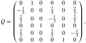
Here, we demonstrate an example realisation of the matrix method for a dendritic structure of three branches of equal lengthx, shown in Fig.2. In this symmetrical case, the matrixQis very small and can be constructed by hand. We place the point of measurementx along edges=(A, B)and the point of current injectiony along
g=(B, D).
We begin by ordering the edge pairs as follows:(A, B),(B, A),(B, C),(C, B),
Fig. 2 A dendritic structure used in the example calculation for the matrix method
one for trips that begin atx and move towardsB, denotedcs1=(1 0 0 0 0 0)T, and another for trips moving fromxtowards nodeA, denotedcs1=(0 1 0 0 0 0)T. Using the rules described in (16), we can construct the matrixQfor our dendritic structure as follows: Q= ⎛ ⎜ ⎜ ⎜ ⎜ ⎜ ⎜ ⎝
0 1 0 0 0 0
−1 3 0 0
2 3 0
2 3 2
3 0 0 −
1 3 0
2 3
0 0 1 0 0 0
2
3 0 0 2
3 0 −
1 3
0 0 0 0 1 0
⎞ ⎟ ⎟ ⎟ ⎟ ⎟ ⎟ ⎠ .
Note that all rows and columns sum to 1. Knowing this matrixQand breaking the trips into four main classes, it is straightforward to find the complete Green’s func-tion:
Gsg(x, y, t )= kmax
k=1
Qk−1cs1gG∞x(2n+x+y), t
+
kmax
k=1
Qk−1c1s
gG∞
x(2n+2−x+y), t
+
kmax
k=1
Qk−1c1sgG∞x(2n+2+x−y), t
+
kmax
k=1
Qk−1c1sgG∞x(2n+4−x−y), t. (18)
4 Convergence of Methods
We first validate the computational implementations of our algorithms by construct-ing the Green’s function Gij(x, y, t ) on a small binary tree. Two profiles of the
[image:15.439.146.294.232.307.2]Fig. 3 The Green’s function constructed by a number of methods. The voltage traces show the analyti-cal solutionsGij(x, y, t )for fixedxandyon a binary tree for the length-priority method (red circles),
the Monte-Carlo method (blue diamonds) and the matrix method withkmax=100 (green squares) su-perimposed on NEURON’s numerical solution (black line). Parameter set A (Table1) is used in these computations
the software package NEURON [26]. These plots demonstrate an excellent agree-ment between a number of approaches for obtaining the Green’s function and the numerical solution, with a slightly worse performance of the Monte-Carlo method for larger times.
The computational convergence of any algorithm impacts both the accuracy of its results and the speed at which these results are obtained. While the series solution to the Green’s function (5) is proven to converge for a sufficiently-high number of terms (see theAppendix), this assumes optimal ordering of terms in the solution. Because the coefficientsAtripare impossible to compute until a trip is constructed,
generating terms for the series solution in descending order of magnitude is inher-ently difficult. The four-classes, length-priority and matrix methods generate trips in order of increasingLtrip, with the aim of ordering trips by theirG∞(Ltrip, t )terms,
which decreases monotonically in the length of the trip. The Monte-Carlo method uses a stochastic method to order trips by their probabilities, with more likely trips contributing more to (5). However, none of these approaches order the trips optimally, and hence their accuracy relies not on the theoretical convergence of the mathematical method, but on the computational convergence of the algorithm that implements it.
[image:16.439.54.388.47.248.2]Fig. 4 Neuronal structures used in construction of the Green’s function.A: a binary tree,B: a rabbit amacrine cell [28],C: a rat pyramidal cell [29],D: a rat Purkinje cell [30], andE: a blowfly tangential cell [31]
using as many nodes as necessary to accurately reflect the spatial jitter and variation in radius of its path. Because radii are described at nodes, edges between two nodes of different radius taper. The sum-over-trips formalism requires constant diameter along edges, but allows discontinuous jumps in the diameters at nodes. Hence, edge diam-eter was defined as the average of the diamdiam-eters of adjacent nodes. This allows full dendritic branches to be represented as a sequence of uniform cylinders of arbitrary length and with abrupt changes in diameters at nodes.
We used the following normalisedL1error as a measure of convergence:
ε= 1 VN
T
0
Gij(x, y, t )−V∗(x, y, t )dt,
whereT is the final simulation time,V∗(x, y, t )is NEURON’s numerical solution to very high accuracy andVN=
T
0 V∗(x, y, t )dt is the integral of the accurate
NEU-RON solution. This convergence measure is therefore relative to the amplitude of the “real” solution, and thus errorsεare comparable between different neuronal types.
[image:17.439.53.388.53.316.2]Fig. 5 Convergence of the four-classes and length-priority methods for a number of dendritic morpholo-gies. The relative errorεof the approximation ofGij(x, y, t )is shown as a function of the number of
trips in the sum-over-trips framework for injection atyand measurement atxon the dendritic trees in Fig.4. Membrane parameters for real dendritic morphologies:C=1 µF cm−2,R=3,000cm2 and
Ra=100cm. Note that the four-classes method always begins with four trips, and each step in the
algorithm adds a further trip of each class
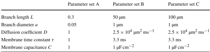
[image:18.439.53.390.47.474.2]Table 1 Parameter sets of the binary tree in Fig.4A
Parameter set A Parameter set B Parameter set C
Branch lengthL 0.3 50 µm 100 µm
Branch diametera 0.05 1 µm 1 µm
Diffusion coefficientD 1 2.5×104µm2ms−1 2.5×104µm2ms−1 Membrane time constantτ 1 3.3 ms 3.3 ms
Membrane capacitanceC 1 1 µF cm−2 1 µF cm−2
Table 2 Length-priority method on a binary tree: number of trips required for a given accuracy
Binary tree Relative error thresholdε
0.1 0.05 0.01 0.001
Parameter set A 3,240 8,750 1,820,000 >5×10⁷ Parameter set B 825 2,600 129,000 >5×10⁷ Parameter set C 22 65 815 7,700
number of trips required on the binary tree to remain under a given error threshold for different parameter sets. Moreover, a binary tree with non-dimensionalised pa-rameters (parameter set A) requires noticeably many more trips for desired accuracy in comparison to the same tree with biophysically realistic parameters.
Figures5D–G showεfor the structures in Figs.4B–E respectively. They demon-strate that convergence is non-trivial on complex branching structures. Figure 5D shows that the length-priority method makes consistently less error on the amacrine cell geometry, in contrast to the convergence of the Purkinje cell, shown in Fig.5E, where the four-classes method generates less error for all numbers of trips. Both of these show strongly irregular convergence and high-amplitude oscillation in the er-rorsεin the amacrine cell. For both methods, the Purkinje cell shows a plateau in error for Green’s functions with few trips, indicating that either these trips are of small magnitude or that their voltage traces alternate between undershooting or over-shooting the correct solution between subsequent trips. This indicates that neither the length-priority or the four-classes methods are good heuristics for ordering terms in the Green’s function. This is further hinted at by the oscillating property of the er-ror, which implies that there are regions where trips that increase the error are more frequent than trips that reduce it.
The pyramidal cell’s convergence shows very discontinuous behaviour (Fig.5F), particularly in the length-priority method. The large jump in error when approxi-mately 350 trips are included in the Green’s function was found to be caused by the first and shortest Class 2 trip included thus far, with all prior trips belonging to Class 1. This behaviour is likely to arise if there exist very short branches along the shortest and most directx→y trip, and thus many Class 1 trips are generated first, being shorter than the first Class 2 trip. Whilst one of the motivating reasons for con-sidering a length-priority approach was to generate trips fully by length order, this heuristic makes no attempt to include the coefficientAtripin its ordering. This is an
which contributes a very significant amount to the Green’s function. The four-classes approach, which enforces generation of trips of all four classes at every added ex-cursion, does not show such a drastic drop in error. However, the error plot is still very discontinuous, and this may be a characteristic of situations as we have just de-scribed, where pointsx andy are placed on branches having a very different length to those on the most directx→y trip, or when these points are placed very close to a node. Whether injection and measurement points are located on branches that are significantly longer or shorter than those along the shortestx→ytrip, both the four-classes and the length-priority methods will generate trips in an “unnatural” order, subsampling the trips where current will spread the most, but oversampling in areas of the tree with very short branches. This pathological feature may not be inherently present in the real neuronal morphology, but may have been created during digital reconstruction from slice image data if, for example, a change of radius were found along the branch. Therefore, this pathology may not be representative of the neuronal geometry, but becomes a function of the reconstruction.
The tangential cell’s convergence, shown in Fig.5G, shows almost identical errors for both the four-classes and the length-priority methods, indicating that trips are generated in a similar order regardless of method. Contrary to the example with the pyramidal cell, this behaviour is likely to occur whenxandyare placed on branches that are significantly shorter than those that arise on the shortestx→ypath, such that the length-priority method returns trips of Class 1, 2, 3 and 4 in sequential order, as these increases in length are shorter than adding an excursion along the directx→y
trip.
Our results clearly indicate that the convergence of the realisation of the sum-over-trips framework by either the four-classes or the length-priority method strongly depends on a dendritic geometry. For real morphologies, the number of trips required quickly becomes very large to the point where guaranteeing convergence to within some small error threshold may become computationally expensive.
The convergence of the Monte-Carlo method is shown in Fig.6for the binary tree in Fig.4A with parameter set A and for a larger binary tree of depth 16 with the same parameters. Boundary effects can be seen on the smaller tree, where the convergence rate is slightly faster than that of a typical Monte-Carlo integration observed here for a larger tree. It is worth noting that thex-axis on this plot shows the number of random walks generated; however, due to the number of sub-trips extracted from each random walk, the number of terms contributing to the Green’s function can potentially be significantly different. The graphs show that the Monte-Carlo method is very slow to converge, although the method is much more predictable in its convergence despite the noise. As expected, therefore, the Monte-Carlo method generates trips that are more “naturally” ordered, and hence convergence is much more monotonic. Despite this improved ordering of terms in the series solution, the Monte-Carlo approach remains computationally intensive and very slow to converge with increased number of trips.
Finally, the convergence of the matrix method on a binary tree is shown in Fig.7. This algorithm converges extremely quickly to within very small error tolerances as a function ofkmax, the maximum number of edges covered by trips generated. The
Fig. 6 Convergence of the Monte-Carlo method for a binary tree. The relative errorε is shown as a function of the number of random walk realisations generated,k.A: error generated on the binary tree in Fig.4A with parameter set A. Thered lineshows a fit forε∼k−0.54.B: the convergence error on a binary tree of depth 16 (65,536 nodes). Thered linedemonstrates a fit forε∼k−0.5, the typical rate of convergence of a Monte-Carlo integration
Fig. 7 Convergence of the matrix method. The relative errorεis shown as a function of the maximal number of edges travelled in the trips,kmax, for a binary tree in Fig.4A
kmaxwhich agrees with the proof in [25]. Because the algorithm is based on simple
matrix-vector multiplication, where the matrix is|E| × |E|in size, the computation of the Green’s function for small trees such as the binary trees used here to within
ε=10−15only takes a fraction of a second. On more complex trees, such as Purkinje cells, this becomes more expensive, although computingGij(x, y, t ) for the whole
tree remains computationally preferable to the use of brute-force simulators. Using the reciprocal rule (9), this is possible in|E|applications of the algorithm. This com-pares favourably with the length-priority and the four-classes methods, which require
[image:21.439.57.389.53.208.2] [image:21.439.79.363.283.453.2]re-quire|E|2simulations, and this would only provide solutions for a single pointy on each edge. In addition, the sparseness of the matrixQmeans that coefficient calcu-lation up tokmaxonly takesO(|E|kmax)time, and so the method scales linearly with
the number of branches on the tree.
4.1 Structural-Electrotonic Properties
The Green’s functionGij(x, y, t )constructed for a given dendritic geometry provides
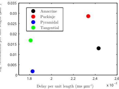
a measure of the transfer impedance between the input locationy on branchj and the point of measurementx on branchi. Assessing whether the neuronal geometry significantly impacts this input-output relation is a step towards answering questions regarding the structure-function relationship behind the enormous natural variation in dendritic morphologies. Using the measures introduced by Zador et al. [32], the propagation delay and the log-attenuation, we analyse the transfer of the response signal in four reconstructed cells in Fig.4. For a pair of points(x, y)along the tree, we reintroduce the propagation delayPxy as a measure of the impact of the tree’s
electrotonic structure on the timing of signals, defined as
Pxy= ˆtx− ˆty.
Here,tˆxandtˆyare the centroids of the two corresponding voltage transientsGx(t )=
Gij(x, y, t )andGy(t )=Gjj(y, y, t )respectively:
ˆ tx=
∞
0 t Gx(t )dt ∞
0 Gx(t )dt
and tˆy=
∞
0 t Gy(t )dt ∞
0 Gy(t )dt .
This delay measure admits an additive property such thatPxy=Pxz+Pzy for a
pointzbetweenx andy. The log-attenuation of the response signal between a pair of points(x, y)is computed asLxy=logAxy>0, where
Axy=
∞
0 Gy(t )dt ∞
0 Gx(t )dt
≥1. (19)
It acts as a measure of the amount a transient signal’s amplitude diminishes as it travels between two points.Lxyis also additive for a pointzbetweenx andy, that
is,Lxy=Lxz+Lzy.
tan-Fig. 8 Propagation delay and log-attenuation for reconstructed geometries
Fig. 9 Transfer properties of the response signal for reconstructed geometries
gential cell having a similar rate of delay with the pyramidal cell and a similar rate of log-attenuation with the amacrine cell. The signal in the Purkinje cell is shown to be attenuated most, whereas the pyramidal cell transfers it very effectively. Similar conclusions, but about the propagation of the dendritic action potential, were made by Vetter et al. [30]. The activation of voltage-gated channels is expected to be less robust in the case of strong attenuation of the passive spread of voltage which might explain the results in [30].
5 Discussion
[image:23.439.53.387.47.191.2] [image:23.439.193.387.227.373.2]nonuniform convergence which was highly-dependent on the dendritic morphology, as well as the biophysical properties of the cell membrane. Oscillations of the con-vergence error make it difficult to predict the number of trips required for construct-ing the Green’s function on a particular geometry. Dendritic structures with longer branches of uniform diameters will converge faster, that is, for a smaller number of trips in the series solution. Instead of sampling the trips in some well-defined order, we also derived a stochastic method of sampling the trips based on a Monte-Carlo ap-proach. Finally, we proposed an extremely efficient matrix method which computes the trip coefficients,Atrip, for trees where all branches are integer-multiples in length
to some base length,x.
Although we considered dendrites to be passive in this study, the proposed al-gorithms can be easily generalised to support quasi-active (resonant) dendrites with a calculation of the Green’s function in the Laplace domain [24]. Moreover, it is straightforward to include an isopotential soma in the Laplace-domain series solu-tion. A soma can be considered as a special node with the factors pk(ω) on the
branches connected to the soma defined as pk(ω)=rk−1
(ω+τ−1)D−1
k /(Cω+
R−1+mrm−1
(ω+τ−1)D−1
m ), whereCandRare the capacitance and the
resis-tance of the somatic membrane andωis the Laplace transform’s frequency variable. Similar factors can also be found for when the leaky-end boundary condition, referred to asnatural terminationby Tuckwell [33], is imposed at the terminals. A knowledge of the Green’s function for a given dendritic structure allows one to efficiently find the sub-threshold voltage response along the entire tree for any number of various inputs, either analytically or via a computation of the convolution integral. This obvi-ates the need for the brute-force numerical simulations of an underlining set of PDEs. Such simulations may be computationally expensive, particularly since they have to be re-initiated each time a new stimulus is introduced. In the case of supra-threshold inputs, which can activate voltage-gated channels known to be present in dendrites of many neurons, the Spike-Diffuse-Spike (SDS) type model [34,35] can be utilised for analysing the propagations of dendritic action potentials. Although the voltage-gated channels in the SDS framework are modelled by piecewise linear instead of nonlin-ear dynamics, it has been shown that the speed of a wave propagation in the SDS model is in excellent agreement with a more biophysically realistic nonlinear model [36]. However, an analytically tractable SDS model combined with a fast algorithm for constructing the Green’s function on real geometries provides a computationally efficient framework for studying wave scattering in dendrites.
of symmetric or regular structures, realistic reconstructions of discretised trees re-main within computational reach. For example, given a sparse random matrix, of correct density and of size 20,000, equivalent to a dendritic tree with 10,000 edges, the calculation ofGij(x, y, t ) for allj up to kmax=105only takes fifteen seconds
on a desktop computer. For comparison, the Purkinje cell reconstruction in Fig.4D has just under 5,000 branches. For the case of very large, complex irregular struc-tures it might be possible to employ a recently developed technique of reducing the complexity of large dendrites [38] before applying the sum-over-trips methodology.
Competing interests
The authors declare that they have no competing interests.
Authors’ contributions
QC was directly involved in developing and implementing the algorithms, carried out all analysis, and drafted the manuscript. SRD participated in developing and implementing the algorithms. SPBC developed the Monte-Carlo algorithm. YT conceived and guided the study. All authors contributed improvements to the final manuscript, which they have read and approved.
Acknowledgements QC and SPCB would like to acknowledge the Complexity Science Doctoral Train-ing Centre at the University of Warwick along with the fundTrain-ing provided by the EPSRC (EP/E501311). SRD acknowledges funding from the EPSRC and the MRC through the Doctoral Training Centre in Neu-roinformatics at the University of Edinburgh. YT would like to acknowledge the support provided by the BBSRC (BB/H011900) and the RCUK.
Appendix: Mathematical Convergence of the Sum-over-trips Series Solution
Here, we consider an identical diffusion coefficientDfor all branches, although it is possible to generalise this proof to support different diffusion coefficients. Fixingt
throughout, we let
Gij(x, y)=
trips
AtripG∞(Ltrip)=
∞
k=0
paths with
knodes
AtripG∞(Ltrip),
where
G∞(Ltrip)=
1
√
4π t De
−L2trip/(4Dt )
e−t /τ. (20)
Atripis a product ofkfactors 2p∈(0,2)and 2p−1∈(−1,1), wherekis the number
of nodes visited by the trip, for any branch diameters. Then, for a trip touchingk
nodes,
|Atrip| ≤2k. (21)
There exists a constantB >0 such that every trip touchingknodes satisfies
This makesBthe coefficient of the lower bound on trip length in terms of the number of nodes in a trip. Intuitively, Bk equals the minimum distance between any two nodes where, for this purpose, we countxandyas nodes.
LetFk be the number of trips withk nodes. Since each node has degreed≤3,
then
Fk≤3k. (23)
We introduce
Γk=
trips with
knodes
AtripG∞(Ltrip).
Then
|Γk| =
trips with
knodes
AtripG∞(Ltrip)
≤
trips with
knodes
AtripG∞(Ltrip)
=
trips with
knodes
|Atrip|G∞(Ltrip). (24)
For simplicity, we rewrite the Green’s function (20) asG∞(Ltrip)=Ce−EL
2
trip, where
C= e
−t /τ
√
4π Dt and E=
1 4Dt.
Then using (21)–(24) we get
|Γk| ≤
trips with
knodes
2kCe−EL2trip
≤
trips with
knodes
2kCe−EB2k2
≤Fk2kCe−EB
2k2
≤3k2kCe−EB2k2
=6kCe−EB2k2
We defineN= ln(6)/(EB2)such thatEB2k−ln(6) >0 for∀k > N. Then
∞
k=0 Γk
≤
∞
k=0 |Γk|
≤∞
k=0
Ce−k(EB2k−ln(6))
=
N
k=0
Ce−k(EB2k−ln(6))+
∞
k=N+1
Ce−k(EB2k−ln(6)). (26)
The first sum in (26) is a finite sum of finite terms, and is hence finite. We will now show that the second sum is also finite using d’Alembert’s ratio criterion for convergent series. The ratioρkof the consecutive terms in the series,kandk+1, is
ρk=
Ce−(k+1)(EB
2(k+1)−ln(6))
Ce−k(EB2k−ln(6))
=e−(EB2(2k+1)−ln(6)).
Lettingk→ ∞, we obtain
ρ∞= lim
k→∞ρk
= lim
k→∞e
−(EB2(2k+1)−ln(6))
=0.
With ρ∞ <1, the second sum in (26) converges absolutely for all constants
B, C, E >0. Therefore, the series in (26) is absolutely convergent for sufficiently-highk.
If we define
GMij(x, y, t )=
M
k=0
trips with
knodes
AtripG∞(Ltrip, t ),
then
Gij−GMij≤
∞
k=M+1
Ce−k(EB2k−ln(6))
References
1. Cajal R:Histology of the Nervous System of Man and Vertebrates. New York: Oxford University Press; 1995 (trans. N Swanson and LW Swanson, first published 1899).
2. Ulfhake B, Kellerth JO:A quantitative light microscopic study of the dendrites of cat spinal alpha-motoneurons after intracellular staining with horseradish peroxidase.J Comp Neurol 1981,202:571-583.
3. Rall W:Core conductor theory and cable properties of neurons. InHandbook of Physiology—The Nervous System (I); 1977:39-97.
4. Segev I, Rinzel J, Shepherd GM (Eds):The Theoretical Foundation of Dendritic Function: Selected Papers of Wilfrid Rall with Commentaries. Cambridge: MIT Press; 1995.
5. Spruston N, Stuart G, Häusser M:Dendritic integration. InDendrites. Edited by Spruston N, Stuart G, Häusser M. New York: Oxford University Press; 2008.
6. van Ooyen A, Duijnhouwer J, Remme MWH, van Pelt J:The effect of dendritic topology on firing patterns in model neurons.Netw Comput Neural Syst2002,13(3):311-325.
7. Spruston N, Stuart G, Häusser M (Eds):Dendrites. New York: Oxford University Press; 2008. 8. Johnston D, Narayanan R:Active dendrites: colorful wings of the mysterious butterflies.Trends
Neurosci2008,31(6):309-316.
9. London M, Häusser M:Dendritic computation.Annu Rev Neurosci2005,28:503-532.
10. Rall W:Theoretical significance of dendritic trees for neuronal input-output relations. InNeural Theory and Modeling. Edited by Reiss RF. Stanford: Stanford University Press; 1964:73-97. 11. Segev I, Fleshmann IJ, Burke RE:Compartmental models of complex neurons. InMethods in
Neuronal Modeling. Cambridge: MIT Press; 1989.
12. Rall W:Theory of physiological properties of dendrites.Ann NY Acad Sci1962,96(2):1071-1092. 13. Koch C, Poggio T:A simple algorithm for solving the cable equation in dendritic trees of
arbi-trary geometry.J Neurosci Methods1985,12(4):303-315.
14. Butz EG, Cowan JD:Transient potentials in dendritic systems of arbitrary geometry.Biophys J 1974,14(9):661-689.
15. Whitehead RR, Rosenberg JR:On trees as equivalent cables.Proc R Soc Lond B, Biol Sci1993,
252(1334):103-108.
16. Lindsay K: Analytical and numerical construction of equivalent cables. Math Biosci 2003,
184(2):137-164.
17. Evans JD, Kember GC, Major G:Techniques for obtaining analytical solutions to the multicylin-der somatic shunt cable model for passive neurones.Biophys J1992,63:350-365.
18. Major G, Evans JD, Jack JJB:Solutions for transients in arbitrary branching cables: I. Voltage recording with a somatic shunt.Biophys J1993,65:423-449.
19. Evans JD, Major G:Techniques for the application of the analytical solution to the multicylinder somatic shunt cable model for passive neurones.Math Biosci1995,125:1-50.
20. Abbott L, Farhi E, Gutmann S:The path integral for dendritic trees.Biol Cybern1991,66:49-60. 21. Cao BJ, Abbott LF:A new computational method for cable theory problems.Biophys J1993,
64(2):303-313.
22. Rapp M, Segev I, Yarom Y:Physiology, morphology and detailed passive models of guinea-pig cerebellar Purkinje cells.J Physiol1994,474:101-118.
23. Eppstein D:Finding the k shortest paths.SIAM J Comput1999,28(2):652-673.
24. Coombes S, Timofeeva Y, Svensson CM, Lord GJ, Josi´c K, Cox SJ, Colbert CM:Branching den-drites with resonant membrane: a “sum-over-trips” approach.Biol Cybern2007,97(2):137-149. 25. Abbott LF:Simple diagrammatic rules for solving dendritic cable problems.Physica A1992,
185(1-4):343-356.
26. Carnevale N, Hines M:The NEURON Book. Cambridge: Cambridge University Press; 2006. 27. Ascoli GA, Donohue DE, Halavi M:NeuroMorpho.Org: a central resource for neuronal
mor-phologies.J Neurosci2007,27(35):9247-9251.
28. Bloomfield A, Miller F:A functional organization of ON and OFF pathways in the rabbit retina. J Neurosci1986,6:1-13.
29. Radman T, Ramos RL, Brumberg JC, Bikson M:Role of cortical cell type and morphology in sub-and suprathreshold uniform electric field stimulation.Brain Stimul2009,2(4):215-228. 30. Vetter P, Roth A, Häusser M:Propagation of action potentials in dendrites depends on dendritic
morphology.J Neurophysiol2001,85:926-937.
32. Zador AM, Agmon-Snir H, Segev I:The morphoelectrotonic transform: a graphical approach to dendritic function.J Neurosci1995,15(3):1669-1682.
33. Tuckwell HC:Introduction to Theoretical Neurobiology: Volume 1. Linear Cable Theory and Den-dritic Structure. Cambridge: Cambridge University Press; 1988.
34. Coombes S, Bressloff PC:Saltatory waves in the spike-diffuse-spike model of active dendritic spines.Phys Rev Lett2003,91:028102.
35. Timofeeva Y:Travelling waves in a model of quasi-active dendrites with active spines.Physica D, Nonlinear Phenom2010,239(9):494-503.
36. Timofeeva Y, Lord GJ, Coombes S:Spatio-temporal filtering properties of a dendritic cable with active spines: a modeling study in the spike-diffuse-spike framework.J Comput Neurosci2006,
21(3):293-306.
37. Harris J, Timofeeva Y:Intercellular calcium waves in the fire-diffuse-fire framework: Green’s function for gap-junctional coupling.Phys Rev E2010,82:051910.

![Fig. 4 Neuronal structures used in construction of the Green’s function.[amacrine cell [ A: a binary tree, B: a rabbit28], C: a rat pyramidal cell [29], D: a rat Purkinje cell [30], and E: a blowfly tangential cell31]](https://thumb-us.123doks.com/thumbv2/123dok_us/9621002.464697/17.439.53.388.53.316/neuronal-structures-construction-function-amacrine-pyramidal-purkinje-tangential.webp)