A quantitative analysis of U S economic development, 1870 1913

(1)

University of Warwick institutional repository:

http://go.warwick.ac.uk/wrap

A Thesis Submitted for the Degree of PhD at the University of Warwick

http://go.warwick.ac.uk/wrap/64233

This thesis is made available online and is protected by original copyright.

Please scroll down to view the document itself.

(2)

A Quantitative Analysis of U.S.

Economic Development, 1870-1913

Author:

Yeo JoonYoon

Supervisor:

Prof. Nicholas Crafts Prof. Anthony _Venables

A thesis submitted for the degree of

Doctor of Philosophy

Department of Economics

University of Warwick

Coventry, United Kingdom

(3)

List of Figures

1 Share of world industrial output . . . 2

(7)

List of Tables

1 Sectoral Employment circa 1870 (in thousand) . . . 30

2 Primary value-added (in wheat units) . . . 30

3 Manufacturing output by major regions . . . 31

4 Britain and U.S. trade in 1870 (in millions) . . . 32

5 Bilateral exports between Britain and U.S. (in millions) . . . 32

6 Calibration targets . . . 33

7 Common parameter values . . . 34

8 Region specific parameter values . . . 34

9 Trade costs . . . 34

10 Social Accounting Matrix . . . 36

11 Trade flows in the benchmark year . . . 37

12 Changes in sectoral TFP . . . 41

13 Changes in endowments . . . 44

14 Changes in trade costs (growth factor) . . . 44

15 Changes in trade costs (growth factor) by Jacks et al. . . 47

16 Residual changes in trade costs (growth factor) . . . 48

17 Simulated results vs. data in 1913 . . . 51

18 Simulated trade output vs. data in 1913 (current prices) . . . 51

19 Simulated results: using the alternative trade cost shocks . . 52

20 Simulated trade output: using the alternative trade cost shocks 53 21 Simulated results under external TFP shocks . . . 54

22 TFP shocks . . . 57

23 Changes in trade costs under CRTS (growth factor) . . . 58

24 Simulated results vs. data in 1913 under CRTS . . . 59

(8)

26 Decomposing trade cost shocks (%) . . . 72

27 Decomposition Using Alternative Trade Cost Shocks (%) . . 73

28 Decomposing contribution of each shock with capital(%) . . . 76

29 Decomposing contribution of each shock under CRTS (%) . . 78

30 Decomposing trade cost shocks under CRTS (%) . . . 79

31 The effects of IRTS on U.S. economy . . . 82

32 Implications of IRTS on U.S. trade . . . 83

33 Static implications of tariffs . . . 97

34 Effects of removing the tariffs on trade and price variables . . 98

35 Sensitivity analysis . . . 100

36 No manufacturing tariffs with learning effects in 1913 . . . . 107

37 Effects of removing the tariffs in 1913 on trade and price variables . . . 108

38 Implications of mass migration . . . 116

39 Implications of mass migration on trade . . . 117

40 Anglo-American real wages . . . 120

41 Implications of the mass migration on real wages . . . 122

42 Decomposition of the changes in real wages . . . 123

43 Real wages with endogenous frontier . . . 127

(9)

Acknowledgements

(10)

Declaration

I declare that the thesis is my own work and has not been submitted for a degree at another university.

Yeo Joon Yoon

(11)

Abstract

The transition of U.S. economy, from a large primary products exporter based on abundant endowments of natural resources to a leading industrial producer and a successful manufacturing exporter from the late 19th cen-tury to the early twentieth cencen-tury, is a remarkable historical event. In this thesis I investigate the quantitative importance of various factors and policies behind the development of the U.S. and the North Atlantic econ-omy from 1870 to 1913. The factors considered are exogenous changes in : sectoral productivities; endowments in labour and land; and trade costs. While these may not be all the factors that mattered, they were certainly important forces behind the development of the region.

I then ask some historically interesting counterfactual questions which are closely related to these forces. First, I explore the implications of the high tariffs imposed on U.S. manufacturing imports. More particularly, I ask “Could U.S. manufacturing and its economy grow as it did without the tariffs?” The second counterfactual exercise is related to the mass migration. There is no doubt that the mass immigration to the U.S. in the nineteenth century contributed considerably to its overall economic growth. But what is uncertain is its quantitative implications on the overall and the sectoral development. I also look at its implications on the Anglo-American real wage convergence.

(12)

Chapter 1

Introduction

1.1 Introduction

1.1.1 Addressing the Question

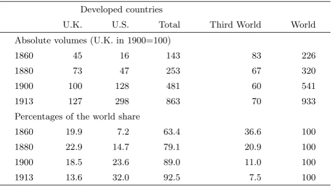
The transition of U.S. economy, from a large primary products exporter based on abundant endowments of natural resources to a leading industrial producer and a successful manufacturing exporter from the late 19th century to early 20th century, is a remarkable event. According to Bairoch (1982), U.S. share of the world manufacturing production in 1860 was only 7.2% but its share surged to 32.0% in 1913. In contrast, U.K share went down from 19.9% in 1860 to 13.6% in 1913. Figure 1 below depicts the relative devel-opment path of U.S. and U.K. manufacturing from 1800 to 1928. From this it can be observed that the growth of U.S. manufacturing accelerated from the mid-nineteenth century, overtaking the U.K. in late-nineteenth century. Also by 1913 the U.S. was the only non-European country in the Atlantic Economy to establish its position as a net manufacturing exporter and rep-resented the third largest share (13.3%) in world manufacturing exports, having net exports of $368 million in 1913 prices (Yates, 1959)

(13)

econ-omy from 1870 to 1913. In doing this I view the phenomenon in an interna-tional context. In other words, I regard the rise of the U.S. and the relative decline of Britain, especially their manufacturing sectors, as a closely related event that happened through interactions of the forces that determined the comparative advantages of each region. For this purpose I build a model that accounts for several key characteristics of the North Atlantic economy - featuring Britain, the U.S. and the rest of world - during the period from 1870 to 1913.

[image:13.595.146.450.285.480.2]

(Source : Bairoch (1982))

Figure 1: Share of world industrial output

Like most of the development experiences of nations or regions, the rise of the U.S. (and the relative decline of Britain) was not an event that can be attributable to one simple cause. It must have been a result of many forces working together. Therefore to evaluate the effect of an individual force, it must be isolated from other forces. And the model briefly mentioned above is built to serve this purpose.

(14)

the U.S. grew substantially relative to the most of other regions including Britain.1 Second, the land area and labour force of the U.S. exploded, mainly due to the westward movement and the mass immigration, respectively. Fi-nally, the changes in trade costs are considered. It is well documented by O’Rourke and Williamson (1999), that the large reduction in transport costs was important in many respects for the North Atlantic economy during this period. But here I do not restrict trade costs to transport costs only. They are perceived as the implied trade costs that include observable as well as unobservable components.2 These forces would have considerable implica-tions under the closed economy framework. But under the open economy framework considered here, they would have additional implications as they shift the comparative advantages among the regions.

The focus is on several dimensions of the development : the large increase in U.S. share of world manufacturing output and the decline in that of Britain; the growth of their primary and manufacturing output and real GDP; and its structural transformation. In order to disentangle the effects of each force, I restrict the model to be consistent with some key facts in the benchmark year of 1870. I then establish that the model accounts for the important developmental facts, just mentioned above, in 1913 when the changes in productivities, endowments and trade costs are fed in. Then the effects of each force on the development of the U.S. are isolated and evaluated by feeding in the change in each force while keeping others unchanged.

The baseline model features increasing returns to scale (IRTS) in manu-facturing, following the evidences that there existed IRTS in U.S. manufac-turing in the late nineteenth century.3 Given the significance of IRTS in U.S. manufacturing, the quantitative implications of this will be investigated. In order to isolate the effects of IRTS, a simple change is made to the baseline IRTS model so that the manufacturing sector now exhibits constant returns to scale (CRTS). It is established that the CRTS model yields identical

cal-1

In the following chapter, the implied changes in sectoral productivities will be mea-sured. Broadberry (1997) and Broadberry and Irwin (2006) clearly establish that the sectoral labour productivities of the U.S. were growing substantially both in absolute terms and relative to Britain during the period.

2

For more discussion of this, see Anderson and van Wincoop (2004).

(15)

ibrated parameter values and equilibrium values in the benchmark year. It is then shown that the CRTS model accounts for the key characteristics of the economy closely when the changes implied by CRTS are fed in. These properties make the two models highly comparable. Then the shocks im-plied by the IRTS model are fed into this otherwise CRTS model. Then by comparing the outcome with that of the baseline model, I disentangle and evaluate the effects of IRTS.

I also ask some historically interesting counterfactual questions which are closely related to these forces. First, I explore the implications of the high tariffs imposed on U.S. manufacturing imports. More particularly, the question I try to answer is “Could U.S. manufacturing and its economy grow as it did without the tariffs?” or put in a more historical context “What if the South had won the War?” The role of tariff in the development of the U.S. in the second half of nineteenth century is still a hotly debated issue among economic historians. I aim to contribute to these literatures by providing some quantitative insights.

The second counterfactual exercise is related to the mass migration. There is no doubt that the mass immigration to the U.S. in the nineteenth century contributed considerably to its overall economic growth. But what is uncertain is its quantitative implications on the overall and the sectoral development. Even though it is not the main focus of the thesis, I also look at its implications on the Anglo-American real wage convergence. This issue is already explored in O’Rourke, Williamson and Hatton (1994) and they find that the contribution of the mass migration on the convergence is quite large. In doing this, they use a standard neo-classical model with constant returns to scale. But the baseline model here assumes IRTS in manufactur-ing, I investigate whether this assumption changes the result quantitatively and qualitatively.

1.1.2 Assumption of the Model

(16)

explanations. The first and foremost important feature of the model is that there exists IRTS in manufacturing. Many previous works studying the economy assume CRTS but at the same time there are arguments and empirical evidences that there was IRTS in U.S. manufacturing during this period.4 Given these evidences, assuming IRTS seems reasonable.

The goal of this thesis is to analyse the factors that contributed to the development of the U.S. and one of the driving forces considered here is the change in productivity, also called the technological progress. But in fact, a large part of this is still a ‘black-box’. In the standard growth accounting exercise, this is treated as a residual which is left unexplained by other observable components. But by assuming IRTS - a reasonable assumption given the evidences - I can reduce the size of the ‘black-box’ and attribute larger parts of the development to more tangible factors. As we will see later in Chapter 2, U.S. manufacturing TFP implied by IRTS is indeed smaller than that implied by CRTS.

One more feature of the model that is closely related to the assump-tion of IRTS is that the manufacturing sector uses manufacturing products as intermediate goods. This basically generates the forward and backward linkage effects, thus inducing the agglomeration of manufacturing when cer-tain conditions are met.5 So this feature helps the model account for the agglomeration of manufacturing in the U.S., without relying on an absurdly large TFP. Crafts and Venables (2001) also argue that IRTS and the linkage effects are needed to replicate the key features of the economy such as the large growth of U.S. manufacturing and constant U.S. to U.K. real wage gap during this period. In addition to this, without this assumption, the implied manufacturing TFP under IRTS becomes identical to that of CRTS. So in a way, this is crucial to distinguish the baseline IRTS model from the CRTS variation.

Next assumption that deserves some explanation is that I do not include capital in the model. According to the estimation of Kendrick (1961), cap-ital increased by more than ten folds during the period for the U.S. And

4

For example see Wright (1990) and O’Rourke and Williamson (1994) for the works assuming CRTS and Chandler (1977), James (1983) and Cain and Paterson (1986) for the works of IRTS.

(17)

there is no doubt that the capital accumulation is one of the important factors for U.S. economic growth from the growth accounting perspective. Capital accumulation is usually treated as an endogenous process. And it is true that a model with an endogenous capital accumulation can yield quan-titatively different results from the outcomes implied by the current model without capital, as the changes in the exogenous forces also influence capital accumulation process as well. But the bottom line here is that the focus of this work is not really on capital accumulation itself. In other words, the model is not focusing on a question such as how the productivity growth or the large increase in land change the pattern of capital accumulation. Besides, including capital in the model complicates things hugely. Also the tractability of the model is not guaranteed as the model needs to become dynamic. Therefore the expense of including capital seems too high given the objectives of the model and I choose simplicity over more realistic re-flection of the history. In several numerical exercises, I include capital in an exogenous manner.

Also even though the model does not include physical capital endoge-nously, it does include land for primary production and manufacturing in-termediate input for manufacturing sector. Land accumulation and capital accumulation are very closely related, especially for U.S. primary sector. According to O’Rourke and Williamson (1994), about 40% of the capital stock in U.S. primary sector was used to improve land in 1870.6 And they argue that this portion of capital is ‘analytically closer to land than capi-tal’. So in this sense including land implies including substantial parts of capital used in the primary sector, if not all. For manufacturing sector, the link between manufacturing intermediates and capital is not so definite as the link between land and capital for primary sector. But one can think of manufacturing intermediate input as a short-lived capital or capital that depreciates fully within a given period. The bottom line is that at least the model includes some form of inputs that are similar to capital in several senses.

6

(18)

1.1.3 Outline of Thesis

The remainder of the paper is organized as follows. In section 2 of this chapter, I summarize the results of Chapter 3, 4 and 5. In section 3 of this chapter, I review the related works. In Chapter 2, I describe the model, the data and the procedure for calibrating parameters and measuring the changes in each force. I then simulate the model to generate the development of the economy from 1870 to 1913 and establish that the model accounts for the history closely. In the last part of Chapter 2, I introduce the CRTS variation of the baseline model. In Chapter 3, I perform a growth decom-position exercise of U.S. economy using the model introduced in Chapter 2. I quantitatively evaluate the impact of each force on the development of U.S. economy. Then in Chapter 4, I study the implications of the tariff imposed on U.S. manufacturing imports. Finally in Chapter 5, I investi-gate the impacts of the mass migration on the development of the U.S. and Anglo-American real wage convergence.

1.2 Results of Chapter 3, 4 and 5

In this section I briefly discuss the outcomes of each chapter. Chapter 2 is designed for the model and the data so there really is no interesting result to talk about. Therefore I begin from chapter 3.

1.2.1 Chapter 3 : Growth Decomposition Exercise

(19)

different approaches of measuring trade cost and TFP shocks and perform similar decomposition exercises. I also include exogenous capital and analyse the contribution of the increase in capital stock.

In the second part of the chapter, I disentangle the effects of IRTS. A caveat regarding this exercise is that it does not evaluate whether the model with IRTS performs better than the CRTS one in accounting for the development of the economy. But it tries to measure the quantitative implications of IRTS assuming that there exists IRTS in manufacturing. The effects of IRTS is not small. This force alone accounts for about one third of the growth in U.S. manufacturing and 10% of the real GDP growth.

1.2.2 Chapter 4 : The Implications of the Tariff

The role of the high tariffs in the development of U.S. economy has generated much controversy. In this chapter I try to add some contributions to this ongoing debate. In order to do this, I perform a counterfactual exercise by eliminating the tariffs on U.S. manufacturing imports. By doing this I can disentangle the effects of the tariff and see its quantitative implications on the development of U.S. economy. The model can serve as a good tool for this purpose.

The overall results suggest that the manufacturing tariffs helped pro-mote its manufacturing sector but its quantitative effects were not so large. Even when I allow for the dynamic and cumulative effects of the tariffs by assuming that there exists learning-by-doing process in U.S. manufacturing, the quantitative effects of the tariffs in promoting the economy are not so large. Under a plausible value of the learning rate, the tariff only accounts for about 3% of the growth in U.S. manufacturing output and less than 1% of the growth in the real GDP.

(20)

1.2.3 Chapter 5 : The Implications of the Mass Migration

Another event that characterises the economy during this period is the mass migration. The massive inflow of immigrants to the U.S. contributed hugely to the increase of its labour forces. The model allows to distinguish the effects of the mass immigration from other forces. In the first part of the chapter I look at the development implications of the immigration. It turns out that the mass migration has quantitatively large impacts on the develop-ment. The net immigration to the U.S. contributes about 12.5% and 26.5% to the growth of primary and manufacturing output, respectively. So the impact is uneven across sectors. When the effects of the net immigration is eliminated, U.S. primary loses 1.6 percentage point in the world share but its manufacturing loses 7.5 percentage point from the world share. Also it accounts for about 20% of the real GDP growth.

(21)

1.3 Related Literatures

The emergence of the U.S. as an industrial power is a remarkable historical event that occurred within such a short span of time. Therefore many studies focused on American economic growth during this period. I begin with those literatures that focus on the role of technology. The modern debate on American ascendancy began with Rothbarth (1946) and Habakkuk (1962). They argued that the relative land abundance in the U.S. raised its real wage rate, thereby increasing the cost of labour for manufacturers. In turn, this induced American entrepreneurs to substitute capital for the dearer labour, leading to a pattern of growth more capital intensive and more rapid than that of Great Britain.7 In their views, the technology developed in the U.S. was only ‘appropriate’ for the conditions in the U.S. thus not optimal to be used in other countries with different endowment conditions. In the same vein, Abramovitz and David (1996) argued that the U.S. developed based on the technology that was intensive in using cheap and abundant natural resources. And for these natural resources were not available to Britain and Europe as cheaply, the technology was not transferable to them.

In a related study, Wright (1990) applied Heckscher-Ohlin model to ex-amine the factor content of trade in manufacturing goods between 1880 and 1940 and drew conclusion that the single most robust characteristic of American manufacturing was intensity in non-reproducible natural re-sources. This result implies that American supremacy in natural endow-ments was important in its industrial success. Hutchinson (2002) supple-ments Wright’s findings using new data from the U.S. Census of Manufac-tures.

A strand of literature also emphasizes the role of institution on the devel-opment of the U.S. In exploring the comparative develdevel-opment trajectory of North and Latin America, Engerman and Sokoloff (1997) argued that initial institutions differed between the two regions because of the different endow-ments with regards to soils, climates and the size of the native population.

7

(22)

More specifically, these conditions in Latin America favoured economic insti-tutions dominated by large-scale estates and plantations which were granted to only small portion of elites. As a result the distribution of wealth and human capital were extremely unequal and opportunities were restricted to the broad mass. On the other hand, the conditions in North America were somewhat opposite to Latin America thus creating institutions that were conducive to lower inequality. And this difference caused the divergent path in the economic development of the two regions. Similarly North, Sum-merhill and Weingast (2000) put forward an argument that the institutions from Spanish colonial rule in Latin America persisted even after ending of the colonialism. And the Latin American institutions contrasted with the North American institutions which were the legacies of British colonialism in the way that the latter promoted a strong sense of property rights and the former didn’t. David and Wright (1997) linked the nature of the Amer-ican institutions that effectively utilized the resource-rich condition to its economic supremacy. For example, they mentioned the role of institutions that promoted and subsidized education and research in the relevant fields such as mining.

In terms of modelling, it is largely based on Krugman and Venables (1995) and Fujita, Krugman and Venables (1999). They introduced the model of New Economic Geography in which the economies of scale and the linkage effects generate the agglomeration of manufacturing in one region. Also closely related is the work of O’Rourke and Williamson (1994). They built a computable general equilibrium model of the North Atlantic economy, calibrated to fit the data. The model, which was based on the standard Heckscher-Ohlin neoclassical framework, was used to study the implications of the global commodity market integration and the reduction in global transportation costs on the factor price convergence. In addition to this, it is also closely in line with the work of Herrendorf, Schmitz and Teixeira (2012) in which they found the large reduction in transportation costs was a quantitatively important force behind the settlement of the Midwest, the regional specialization and the increase in real GDP per capita in the U.S. from 1840 to 1860.

(23)

signif-icance of the scale economy in U.S. manufacturing. First, Chandler (1977) argued that the capital deepening technological change, that was apparent in the late nineteenth century U.S. manufacturing, generated the economies of scale and this made possible the dramatic rise of the industry in the world stage. James (1983) and Cain and Paterson (1986) tested this argument empirically by estimating the translog production function and documented that the economies of scale in U.S. manufacturing were substantial and per-vasive in the late nineteenth century.

Cain and Paterson (1986) use the Generalized Leontief production func-tion to derive real factor demand equafunc-tions.8 Using this, they simultaneously test the presence of economies of scale, biased technical change and factor substitutability in U.S. manufacturing at the two digit level in the years from 1850 to 1919. The result shows the evidence of the economies of scale in U.S. manufacturing during the period. Out of 19 manufacturing sectors, only two sectors, food and beverage (SIC 20) and leather goods (SIC 31), are found to exhibit constant returns to scale technology. The presence of economies of scale in the other 17 sectors was more attributable to capital than labour.

James (1984) tests the hypotheses of Chandler (1977) that the rise of U.S. manufacturing was mainly due to the labour-saving and capital-intensive technological change which, in turn, made possible the development of large firms and big business. Even though its main objective is to examine the relationship between capital-biased technological change and changes in re-turns to scale, it also establishes that there existed a significant degree of scale economy and the range of economies of scale increased substantially in 16 manufacturing sectors during the periods between 1850 and 1890. Fi-nally, Atack (1977) estimates a Cobb-Douglas production function for 5 ma-jor manufacturing sectors - boots and shoes, clothing, cotton, flour milling and lumber milling - in the antebellum year of 1850 and 1860. He establishes that there existed substantial economies of scale in U.S. manufacturing and

8_{The equation looks like} _A

(24)

the range increased from 1850 to 1860.

There are ample empirical evidences that support the presence of scale economies in U.S. manufacturing in the late nineteenth century. However as to whether this was internal or external economies of scale or a combination of both, it is not so clear while this obviously affects my modelling choice. As it will be more clear when I introduce my model in Chapter 2, I assume that it is internal economies of scale. The implications of this assumption will be discussed more in detail in Section 2 of Chapter 3.9

9

(25)

Chapter 2

The Model and the Data

2.1 The Baseline Model

A benchmark model is constructed to account for some important charac-teristics of the U.S. and the North Atlantic Economy in the late nineteenth century. I consider factors that potentially could have been important forces driving the outcome: differences in sectoral productivity or TFP, trade costs and endowments.10

The economy consists of 3 regions : Britain, the U.S. and the rest of the world. Each region has 3 sectors of production : primary, manufac-turing and services. Primary and manufacmanufac-turing goods are tradable while goods produced in the service sector are non-tradable. There are 3 factors of production : land, labour and manufacturing intermediates. The pri-mary sector uses land and labour, the manufacturing sector uses labour and manufacturing intermediates and the service sector only uses labour.11 The manufacturing sector exhibits increasing returns to scale at the firm level

10_{Obviously, the Heckscher-Ohlin model assumes a common technology across regions}

but differences in sectoral productivity in levels and in growth were significant between two regions (Broadberry, 1997).

11

(26)

while the other sectors have constant returns to scale.12 Labour is perfectly mobile across sectors so that wages are equalized across sectors. Basically the model obeys the standard assumptions of the New Economic Geography literature.

2.1.1 Consumer Behaviour

There is a measure Di > 0 of identical consumers. Every consumer shares

the same Cobb-Douglas tastes over the three types of goods,

U = (cai−ci) θa_cθm

mic θs si

where cai and cmi represent composite indexes of the consumption of

pri-mary and manufactured goods, respectively, and ci is the subsistence level

of consumption in primary andi={b,us,rw}. The indexcai is a sub-utility

function defined over differentiated agricultural products that each region produces. Likewisecmi is defined over a continuum of varieties of

manufac-tured goods:

cai=

h γba

ρa

i,b+γusaρi,usa +γrwaρi,rwa

i1/ρa

, cmi =

Z n

0

m(j)ρm_dj

1/ρm

whereai,j represents regioni’s demand for region j’s primary products and

m(j) represents manufacturing consumption of each available variety. n is the total number of manufacturing varieties produced in all three regions. This specification yields the price indexes forcai and cmias

Gai=

γσa

b (pa,bTbia)1−σa+γusσa(pa,usTusia )1−σa+γrwσa(pa,rwTrwia )1−σa

1/(1−σa) (1)

Gmi=



 X

j

nmj(pmjTjim)

1−σm





1/(1−σm)

(2)

12_{Later in the paper the assumption of increasing returns will be relaxed and some}

(27)

wherepa,iis the price of a primary good produced iniandTjiaandT m

ji are the

iceberg transportation costs of agriculture and manufacturing from region

j to i respectively; σa = ₁−1ρa and σm =

1

1−ρm. γi is the share parameter

and the meaning of this parameter will be discussed more in detail in later in this chapter where I go over the calibration procedure.

2.1.2 Production

The primary good is produced using a constant returns to scale technology under perfect competition. It uses land and labour as inputs and has a production function as

Yai =Aai(Lai)αa(Nai)

1−αa

whereLai is labour, Nai is land andAai is TFP. Cost-minimization implies

the following condition,

pai= Γaω_iαad1_i−αa (3)

wherepai is the price of the primary good,ωi is the wage anddiis land rent;

Γa= (Aaiααaa(1−αa)1−αa)−1.

I assume the manufacturing sector exhibits IRTS. As in Krugman and Venables (1995), these economies of scale arise at the level of a firm and technology is the same for all firms in all regions and involves a fixed input of F. I also assume that in addition to labour, it uses its own produced variety. Its production function can be defined as

Ymi=Ami(lmi)αm 

 X

j

nmjm ρm ji





(1−αm)/ρm

−F

whereAmi is TFP,mji is input of each manufacturing variety produced in

(28)

region j. lmi is labour employed by a single manufacturing firm in region

i. It should be distinguished from an upper-case letter Lmi which denotes

the aggregate amount of labour employed in regioni’s manufacturing sector that will appear shortly.

The underlying assumption is that the elasticity of substitution among differentiated products for manufacturing firms is the same as that for con-sumers as they share the same ρm. In other words, this implies that firms

and consumers in each region face the same manufacturing price index. This assumption would not be central to my results because the results are not sensitive to the elasticity of substitution parameters but this makes anal-ysis much more tractable and manageable. Cost minimization implies the following,

ωilmi+GmiMi= ΓmiωiαmG

1−αm

mi (Ymi+F) (4)

where Γmi= (Amiααmm (1−αm)

(1−αm)₎−1 _and _M

i = h

P

jnmjm ρ ji

i1/ρ

.

The service sector, like the primary sector, uses a constant returns to scale technology under the perfect competition and uses labour as its only input. Its production technology can be described as,

Ysi=AsiLsi

and profit maximization implies,

psi =

ωi

Asi

(29)

2.1.3 Demand

The demand for manufacturing goods can be decomposed into two parts: final goods or consumption demand and intermediate demand. The aggre-gated world demand for a manufacturing good produced in region iis

(pmi)

−σm



 X

j

θm(Yj−CiGaj)

_Tm ij

Gmj

1−σm +X

j

(1−αm)nmjpmjqmj

_Tm ij

Gmj

1−σm

 (6)

where C_i = Di ci. The first term is the world consumption demand and

the second term is the world intermediate demand. Yj represents income of

regionj and qmj is sales of a manufacturing firm in regionj that is in line

with the zero-profit condition. Using (6) and profit maximization, the price index for the composite manufacturing good, pmi, can be derived and qmi

can be obtained by imposing the zero-profit condition.

pmi =

σm

(σm−1)

Γmi ωαmi G

1−αm

mi (7)

qmi=F(σm−1) (8)

It is easier to obtain the demand for primary goods as it is only used in consumption. The world demand for a primary good produced in region i

is

X

j

[θa(Yj−CiGaj) +CiGaj] (pai)

−σa _Ta

ij

Gaj 1−σa

(9)

Finally, the demand for a non-tradable service good in regioniis

θa(Yi−CiGai)

psi

(30)

2.1.4 Reformulation

In this section, I reformulate the equations in order to define the equilibrium in a simpler way. Primary and service expenditure of region i only come from final consumption while manufacturing expenditure comes from final consumption and intermediate usage. Therefore, regioni’s expenditures are given by

Eai = θa(Yi−Ci Gai) +CiGai (11)

Emi = θm(Yi−CiGai) + (1−αm)nmipmiqmi (12)

Esi = θs(Yi−CiGai) (13)

The second term on the right hand side of (12) is intermediate demand. Wage income in the manufacturing sector, ωiLmi (Lmi is total labour

force in the manufacturing sector) is equal to the total value of manufactur-ing output times the share of labour, αmnmipmiqmi. The number of

manu-facturing firms can be expressed as

nmi=

ωiLmi

αmpmiF(σm−1)

(14)

Using (7) and (14), the manufacturing price-index (2) can be expressed in terms of wage and allocation,

(Gmi)

1−σm ₌X j

BjLmj(ωj)

1−αmσm₍_G mj)σm

(αm−1)

(Tm ji)

1−σm ₍₁₅₎

where Bj = (αmF σσmm(σm−1)(1−σm)Γσmjm)

−1

. Substituting (3) into (1), the pri-mary price-index can be re-written as

(Gai)

1−σa ₌X j

γσa j Γ

1−σa aj (ωj)

αa(1−σa)₍_d

j)(1−αa)(1−σa)(Tjia)

(31)

The service-price index is the same as in (5) :

psi=Gsi =

ωi

Asi

(17)

I reformulate the goods market clearing conditions in terms of expendi-tures (Ei), price-indexes (Gi) and wage (ωi). First, for the primary sector

in each region to clear,Yai has to equal (9). Using (3) and (11), I have

Γa(ωi)αa(di)

1−αa

γi

σa

Yai = X

j

Eaj _Ta

ij

Gaj 1−σa

(18)

Likewise for the manufacturing sector, (8) has to be equal to (6). Using (7), (12) and (14), it can be expressed as,

Ci ωαmσmi (Gmi)

(1−αm)σm ₌X j

Emj

Tm ij

Gmj 1−σm

(19)

whereCi=F σσmm (σm−1)

(1−σm)_Γσm

mi. Finally, using (10), (13) and (17), the

goods market clearing condition for the service sector can be given as,

ωiLsi =Esi (20)

Total endowment of labour in each region is given as L_i and the labour market clearing condition is

L_i=Lai+Lmi+Lsi (21)

Total endowment of land in each region isN_i and the land market clearing condition is

(32)

Finally, the income of each regioniis

Yi=ωiLi+diNi (23)

Two additional equations are required to define the equilibrium. They are factor demands for land and labour in the primary sector.

Ni =

1

Aai

1−αa

αa

ωi

di

αa

Yai (24)

Lai=

1

Aai

αa

1−αa

di

ωi

1−αa

Yai (25)

2.1.5 Equilibrium

The general equilibrium determines each region’s wage and land rent: {wi,

di}, land and labour allocations: {Ni, Lai, Lmi, Lsi}, price-indices: {Gai,

Gmi, Gsi}, expenditures: {Eai, Emi, Esi}, agricultural output {Yai}, and

income: {Yi}. The expenditure equations (11)-(13), price-index equations

(15)-(17), goods market clearing equations (18)-(20), labour and land mar-ket clearing equation (21)-(22), income equation (23) and factor demand equations (24)-(25) constitute 14 equations to solve for 14 unknowns for each region. Obviously there are three regions so that makes 42 equations with 42 unknowns.13

I use Matlab to solve this system of equations. It does not guarantee a unique solution as the New Economic Geography model typically has multiple equilibria. However I tried many different initial values and they all converged to the same equilibrium. The parameters are calibrated to match

13_{In this system of equations, the outputs for other sectors,}_Y

(33)

various features of the economy during this period. A detailed description of the calibration procedure is discussed in the following section and in the appendix of Chapter 2.

2.2 Restricting the Model Parameters

In this section I restrict the parameters of the model to make them con-sistent with some key characteristics of the economy circa 1870, along with detailed descriptions of data. Essentially, I need to calibrate the following parameters. The region specific preference parametersγi fori={b,us,rw},

c, θa, θm and θs; the TFP parameters Aai, Ami and Asi for each region;

the endowmentsN_i andL_i for each region; the elasticity parametersσaand

σm which are common across regions; the production share parameters αa

and αm which are common across regions; the fixed cost in manufacturing

production and the amount of production by a single firmF; and the trade costsTija and T

m ij

2.2.1 Classification

Tradeables are classified according to the Standard International Trade Clas-sification (SITC, revision 4). Products under section 0, 1, 2 and 4 are clas-sified as primary good and under section 3, 5, 6, 7 and 8 are clasclas-sified as manufacturing good.14 So basically food products (processed or unpro-cessed), raw materials or materials in crude state and products from farm are included in primary sector.

For sectoral output, due to limited availability of disaggregated data, I do not classify them using raw data. But rather I take them from other

14_{Section 0-food and live animals; section 1-beverages and tobacco; section 2-crude}

(34)

sources, mainly from Bairoch (1982), Broadberry and Irwin (2006) and Federico (2004). Their classifications are very similar to the conventional system based on International Standard Industry Classification (ISIC) or North American Industry Classification System (NAICS). Primary sector includes farming, fishing and forestry and manufacturing sector includes mining, manufacturing and construction.15

Discrepancies necessarily arise between the definition of tradeable goods and of sectoral output, given the way they are classified. Basically, trade-able items are classified based on the characteristics of products whereas industries are classified based on the characteristics of production activities. For example, in my model, the food processing industry is included in man-ufacturing but the processed food itself is classified as a primary tradeable. This is reasonable as processed food contains disproportionately more value accrued from the primary activities (farming, fishing and so on).16

2.2.2 Gross Output or Value-added?

In the model manufacturing output of region i, Ym,i, corresponds to gross

output rather than to value-added. More specifically, Ym,i is gross output

only including manufacturing intermediate inputs. Broadberry and Irwin (2006), one of the sources which I use to construct these figures, define manufacturing output in terms of value-added. Bairoch (1982) does not clearly specify whether they are value-added or gross output. Given the limited data availability, each region’s manufacturing output data reflecting gross output are not available.

The model however implies that the value-added is a fixed proportion of the gross output. Real value-added in manufacturing of region ican be

15_{Engineering and metal manufactures; textiles and clothing; food, drink and tobacco;}

paper and printing; chemicals; wood industries; miscellaneous manufactures

16_{According to the U.S. Census, in 1869 the gross output in the food processing industry}

(35)

defined as

Real value added = pm,iYm,i−Gm,iMi

pm,i

where Mi is manufacturing intermediate input. The equilibrium condition

implies thatGm,iMi= (1−αm)pm,iYm,i. Plugging this into the above equation,

the real value-added is αmYm,i. When it comes to the relative terms, the

model implies there is no difference between gross output and value-added.17

2.2.3 Normalization

Several normalizations are in order. To begin with, θa+θm +θs = 1 for

each region andγb+γus+γrw = 1. Moreover, I normalize the TFPs, land

and labor endowments in Britain: Aa,b = Am,b = As,b = Nb = Lb = 1. I

also normalize domestic trade costs to 1, so Tiia = T m

ii = 1. The choice of

F, the fixed cost in manufacturing sector, proportionally scales up or down the number of firms in these industries, but leaves the values of all other aggregate variables unchanged in a relative sense. Therefore I can normalize them to arbitrary numbers and I setF = 0.1. F affects the economy through the zero-profit production level of a single manufacturing firm in equation (8) and the number of manufacturing firms in regioniin equation (14). Of course different values ofF yield different absolute values ofqmiandnmibut

as long asF is equal across regions, the relative values are not affected by the choice ofF including the manufacturing price-index. I am mainly interested in the relative performance of U.S. economy (in terms of its growth over the periods and its performance relative to Britain), the relative values only matter. Also in the sense that it does not affect the relative price levels, it does not affect the relative real wages which will be the focus of Chapter 5.18

17_{Of course this comes from the underlying assumption that}_α

m is constant across

re-gions. As we will see shortly, I am mostly interested in relative terms such as U.S. manufac-turing output relative to Britain’s output,Ym,us/Ym,bor the growth factor,Ym,b,1913/Ym,b,1870.

18

(36)

ex-2.2.4 Parameters I Calibrate Individually

σa and σm : the elasticity of substitution

I start with σa and σm which are the elasticity of substitution in primary

and manufacturing products, respectively. According to Anderson and van Wincoop (2004), it is likely to be in the range of 5 to 10. So initially I choose 7.5 for both. Later, in a sensitivity analysis, I vary these values within this range to see how sensitive the results are.

L_i and N_i : endowments

I continue with the endowments of land and labour force in each region. Feinstein (1972) reports the total labour force for Britain in 1870 is 13,950 thousands and Kendrick (1961) reports it for the U.S. in 1869 as 11,910 thousands. Therefore the share of U.S. labour force relative to Britain’s is about 0.85. Given the normalizationL_b = 1, I setL_us = 0.85. Employment data for the rest of world circa 1870 is incomplete therefore I infer world population from Maddison (2001) to calibrateL_rw. The rest of world popu-lation is about 40 times larger than Britain’s, so I assign L_rw=40. Abstract of British Historical Statistics and the U.S. Census of Agriculture reports land usage for Britain and the U.S., respectively. According to them, land usage in the U.S. in 1870 is about 4 times larger than that of Britain, so I setN_us = 4 givenN_b = 1.19 Again, land usage data for the rest of world is incomplete, so I assignN_rw = 40.20

hibits different degree of IRTS. This, however, is not a possible option under the current methodology because then the model solving procedure can get immensely complicated. Certainly this would be an interesting possibility to consider in many aspects including the real wage convergence story to be covered in Chapter 5. In this case I would need more realistic choice ofF to reflect the difference in the degree of IRTS across regions.

19

According to the Historical Statistics, 46,018 thousands acres of land was used for crops and pasture in Britain in 1870. TheCensus reports that 188,921 thousands acres of ‘improved land’, the classification which corresponds to the land usage in Britain, was used for the U.S.

20

Indeed,Lrw only influences the equilibrium value ofdrw and the calibrated value of

(37)

αa : the share of labour in the primary sector

Next, I continue with the share parameters in primary and manufacturing production. As these parameters are assumed to be common across regions, I take the arithmetic average of each region’s share. I start with the share of labour in primary sector. For Britain, O’Rourke and Williamson (1994) calculate the share of wage income in the primary sector in 1871 as 0.53. Clark (2010) estimates the share of farm capital and land income in total farm income for 1860-1869 as 0.48. If I take the residual as farm wage income then the share is 0.52, so they yield almost identical share parameter values. For the U.S., O’Rourke and Williamson (1994) calculates the share of capital and land income as 0.41 and in turn, the wage income share is 0.59. I use Sweden as a proxy for the rest of world as it is almost impossible to get all the data needed. According to Edvinson (2005), the labour income share in 1870 is 0.69. And by taking the average of these numbers, I setαa= 0.6.

Admittedly, it may be too much of a generalization to say that Sweden is a perfect representation of the rest of world circa 1870. But without loss of generality, we can say that Sweden can be a sensible approximation because it was a relatively more labour intensive economy than Britain or the U.S. circa 1870. And given data availability, Sweden is a plausible proxy for the rest of world in calibrating the labour share parameter.

αm : the share of labour in manufacturing sector

Next I move to the share parameter in manufacturing sector. Here I pin down the share of manufacturing intermediates, 1−αm, and take the share

(38)

specifi-cation. Manufacturing sector in my model does not include primary and service intermediate goods, therefore gross output is defined as value-added plus manufacturing intermediates only. Then 1−αm is obtained using this

new measure of the gross output.

For Britain, there are input-output table for 1851 and 1907 constructed by Thomas (in progress) and Thomas (1984), respectively. I take the average of the values implied by these two input-output tables. In 1851, the share of labour turns out to be around 0.6 and in 1907, 0.49. So for Britain it is about 0.55. For the U.S., the only available input-output table is for 1899, constructed by Whitney (1968). And it yields a labour share of 0.53. For the rest of world, which is again proxied by Sweden, I use an input-output table for 1885 by Bohlin (2007) which estimates the labour share as 0.66. By taking the average, I setαm= 0.58.

γi : the weight on consumption of primary products from region i

Next, I calibrate γb, γus and γrw which are assumed to be equal across

re-gions. The conventional way to calibrate γi parameters is to fit these to

the expenditure share of goods from each region (for example, the share of imported products from Britain in U.S. total primary expenditure). This, indeed, is what the utility function implies. This approach is typically used in the standard computational general equilibrium (CGE) model. This, however, means thatγis are not equal across regions (For example I would

need to calibrate γus,i instead of γus that indicates the share of imported

(39)

as-sume that γis are equal across regions. I calibrate these parameters using

the price index equation (1). To draw a meaningful interpretation of γis,

I compare equation (1) to equation (2), the manufacturing price index. In this equation the counterpart ofγi isnmi which corresponds to the number

of manufacturing firms in regioni. This defines the distribution of manufac-turing varieties (activities) across regions. We can think of γi in the same

manner. In other words, the number of varieties produced in a region is proportional to the volume of primary goods produced in that region. In my case, the rest of world which is the biggest producer of primary goods also produces the largest number of varieties.21 The only difference between the two is that γi is fixed or exogenous whereasnmi is endogenously

deter-mined. Fujita, Krugman and Venables (1999) takes this approach when they assign values to these parameters. I use each region’s share of world primary production as estimated by Federico (2004) to pin down these values.

As,i : TFP for region i’s services sector

Next, the TFPs for services sectors are calibrated. Broadberry and Irwin (2006) estimate that U.S. labour productivity in the services sector is 0.77 given that of Britain is 1. So I setAs,us= 0.77. For the rest of world, I set

As,rw = 0.5 arbitrarily. The overall results are not sensitive to this value

because the services sector is a residual sector that produces non-tradable goods. The rest of world is not the focus in this paper anyway and the non-tradable service sector of this region has small impacts on primary or manufacturing sector of the U.S. or Britain which are the main focuses.

21

For comparison I report the values ofγs that match the expenditure shares of Britain and the U.S. γi,j denotes the share of imported products from j in i’s total primary

expenditure : γus,b = 0.00, γus,us = 0.95, γus,rw = 0.05,γb,b = 0.67, γb,us = 0.09 and

(40)

Di : measure of region i’s consumer

This parameter only controls C_i = Di ci in the aggregate equilibrium. I

use the population of each region to proxy this. I normalize Db = 1 then

according to Maddison (2001),Dus= 1.37 and Drw = 40.

2.2.5 Parameters I Calibrate Jointly

At this point, I am left with 27 parameters. 12 trade costs: Ta ij and T

m ij, 9

preference parameters: θa,θm and C for each region and 6 TFPs: Aa,i and

Am,i for each region. I choose them such that the model replicates key

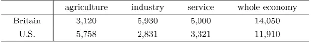
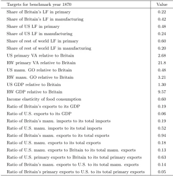
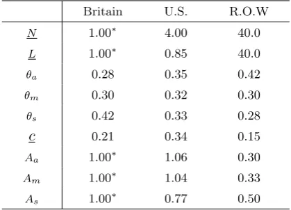
char-acteristics of the benchmark year economy circa 1870. Specifically, I target: (1) the shares of each region’s labour forces in each sector as reported; (2) each region’s primary and manufacturing value-added relative to Britain; (3) each region’s nominal GDP relative to Britain; (4) the income elasticity of demand for food estimated by various sources; (5) Britain and the U.S. exports to GDP ratio in current prices; (6) the ratio of Britain’s and U.S. manufacturing imports to their total imports; (7) the ratio of Britain’s and U.S. manufacturing exports to their total exports; (8) the ratio of Britain’s primary and manufacturing exports to the U.S. to its total primary and manufacturing exports, respectively; (9) the ratio of U.S. primary and man-ufacturing exports to Britain to its total primary and manman-ufacturing exports, respectively. Below I provide a detailed description of data and algorithm of the calibration procedure.

(1) The share of labour in each sector

(41)

[image:41.595.139.456.162.205.2]

Table 1: Sectoral Employment circa 1870 (in thousand)

agriculture industry service whole economy

Britain 3,120 5,930 5,000 14,050

U.S. 5,758 2,831 3,321 11,910

Source: see the text

(2) Sectoral output relative to Britain

For each region’s value-added in the primary sector, I rely on Federico (2004). He includes 49 countries and 23 products that account for more than 70% of the world primary output. He measures relative prices for these products in terms of wheat with which he obtains PPP-adjusted value-added for these countries for 1913. In order to obtain the figures for 1870, I use the volume indices that he provides from 1800 to 1938. Table 2 below re-ports the primary value-added of each region in 1870 and 1913 with which I construct value-added relative to that of Britain.

Table 2: Primary value-added (in wheat units)

in 1913 in 1870

Britain 17,152 18,387

U.S. 127,031 49,288

World 884,124 468,586

Source: see the text. Note: volume-index in 1870 was 107.2, 38.8 and 53.0 for Britain, U.S. and the world, respectively with 1913=100.

(42)

[image:42.595.135.461.161.344.2]

Table 3: Manufacturing output by major regions

Developed countries

U.K. U.S. Total Third World World

Absolute volumes (U.K. in 1900=100)

1860 45 16 143 83 226

1880 73 47 253 67 320

1900 100 128 481 60 541

1913 127 298 863 70 933

Percentages of the world share

1860 19.9 7.2 63.4 36.6 100

1880 22.9 14.7 79.1 20.9 100

1900 18.5 23.6 89.0 11.0 100

1913 13.6 32.0 92.5 7.5 100

Source : see the text

(3) Nominal GDP relative to Britain

Officer and Williamson (2010) provide nominal GDP for Britain and the U.S. in domestic currencies. I use the bilateral exchange rates, from the same source, to convert the GDPs in U.S. dollar. For the rest of world, as nominal GDP is not available, I rely on Maddison (2001) which reports the world’s and each region’s GDP in Geary-Khamis international dollars. I can then subtract the Britain and U.S. GDP from world GDP to obtain the rest of world GDP (relative to Britain).

(4) Income elasticity of demand for agricultural output

(43)

turns out to be about 0.607 for industrial workers, 0.570 for skilled workers and 0.730 for unskilled workers. Given these, the most plausible value seems to be around 0.6 and I rely on this value in my model.

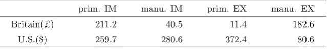
(5)-(9) Trade data

[image:43.595.138.459.453.501.2]

Basically all the trade data are taken fromthe Annual Statement of Trade of the United Kingdom and Annual Report of the Commerce and Naviga-tion of the United States. I classify each good traded into either primary or manufacturing according to the classification rule described above. Ta-bles 4 and 5 below describe the trade statistics constructed for calibration. Finally, Table 6 summarizes the targets and their values. In the appendix I provide a detailed description of the joint calibration procedure. Table 7 summarizes the parameters common across regions, Table 8 summarizes the region specific parameter values and Table 9 reports the trade costs.

Table 4: Britain and U.S. trade in 1870 (in millions)

prim. IM manu. IM prim. EX manu. EX

Britain(£) 211.2 40.5 11.4 182.6

U.S.($) 259.7 280.6 372.4 80.6

Note : Imports(IM) defined here are net-imports which are as imports - re-exports. U.S. imports and re-exports are in gold-terms, so I convert them into currency terms using an exchange rate of $1=0.742 gold$ as in O’Rourke and Williamson (1994).

Table 5: Bilateral exports between Britain and U.S. (in millions)

primary exports manufacture exports

Britain to U.S.(£) 0.5 25.9

[image:43.595.149.446.593.640.2]

(44)

[image:44.595.118.474.147.512.2]

Table 6: Calibration targets

Targets for benchmark year 1870 Value

Share of Britain’s LF in primary 0.22

Share of Britain’s LF in manufacturing 0.42

Share of US LF in primary 0.48

Share of US LF in manufacturing 0.24

Share of rest of world LF in primary 0.60

Share of rest of world LF in manufacturing 0.20

US primary VA relative to Britain 2.68

RW primary VA relative to Britain 21.8

US manu. GO relative to Britain 0.48

RW manu. GO relative to Britain 3.21

US GDP relative to Britain 1.30

RW GDP relative to Britain 9.57

Income elasticity of food consumption 0.60

Ratio of Britain’s exports to its GDP 0.19

Ratio of U.S. exports to its GDP 0.06

Ratio of Britain’s manu. imports to its total imports 0.19

Ratio of U.S. manu. imports to its total imports 0.52

Ratio of Britain’s manu. exports to its total exports 0.94

Ratio of U.S. manu. exports to its total exports 0.18

Ratio of U.S. manu. exports to Britain to its total manu. exports 0.13

Ratio of U.S. primary exports to Britain to its total primary exports 0.63

Ratio of Britain’s manu. exports to U.S. to its total manu. exports 0.14

Ratio of Britain’s primary exports to U.S. to its total primary exports 0.05

(45)

Table 7: Common parameter values

σa σm αa αm F γb γus γrw

[image:45.595.192.402.248.399.2]

7.5 7.5 0.6 0.58 0.1 0.04 0.10 0.86

Table 8: Region specific parameter values

Britain U.S. R.O.W

N 1.00∗ 4.00 40.0

L 1.00∗ 0.85 40.0

θa 0.28 0.35 0.42

θm 0.30 0.32 0.30

θs 0.42 0.33 0.28

c 0.21 0.34 0.15

Aa 1.00∗ 1.06 0.30

Am 1.00∗ 1.04 0.33

As 1.00∗ 0.77 0.50

* indicates normalization.

Table 9: Trade costs

Ta b,us T a b,rw T a us,b T a

us,rw Trw,ba T a

rw,us Tb,usm T m b,rw T

m us,b T

m

us,rw Trw,bm T m rw,us

2.38 1.64 1.74 1.85 1.91 2.05 2.30 1.48 1.56 1.45 1.53 2.56

Conventionally, most of the trade cost literature assumes symmetric trade costs between two regions.22 But from Table 9, it can be seen that the calibrated trade costs yield quite large asymmetries between the U.S. and other regions with a larger asymmetry for manufacturing goods. One of the factors that can explain this discrepancy around 1870 is the trade policy. It is well-know that the U.S. erected high barriers on its imports in order to protect its industry during this period. On the other hand, Britain was essentially a free trade country. Therefore this difference must have

22

(46)

contributed to a significant extent to the asymmetry observed in the table. More on this issue will be discussed in the following chapters.

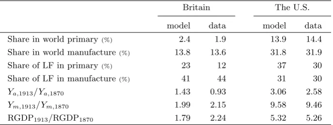
One thing to note is that even though I do not target the model to match the real GDP of the U.S. relative to Britain, the implied values match the data quite closely. Real GDP can be defined as

Real GDP = Y

Gθa

a Gθmm Gθss

where the regional subscriptihas been dropped. The term in the denomina-tor can be interpreted as a price-index. The implied ratio of U.S. real GDP per capita to that of Britain is about 0.97. Maddison (2001) suggests that this ratio is about 1.03 when measured in 1990 Geary-Khamis international dollar.

Next I demonstrate that the benchmark year equilibrium generated by the calibration is internally consistent - expenditure plus net exports, gross output and factor costs of each region are equalized and trades are balanced. To do this I construct a Social Accounting Matrix (SAM) in the benchmark year of 1870 implied by the model. Table 10 below presents the SAM. Note that the value of U.S. primary gross output is normalized to 1 and all other values are in relative terms.

First, the model correctly predicts that the U.S. is a net exporter of primary product while being a net importer of manufacturing product (and vice versa for Britain). The table shows that the value of each region’s gross output in each sector is equal to the value of net exports plus expenditure (GO = Expenditure + NX). It also shows that the trades are balanced in each region (NX across sectors in each region add up to zero).

(47)

[image:47.595.116.482.162.402.2]

Table 10: Social Accounting Matrix

Industry GO Input Cost VA NX Expenditure

L N M

U.S.

P 1.00 0.60 0.40 1.00 0.03 0.97

M 0.52 0.30 0.22 0.30 -0.03 0.55

S 0.35 0.35 0.35 0.35

Total 1.87 1.25 0.40 0.22 1.65 0.00 1.87

Britain

P 0.41 0.24 0.16 0.41 -0.18 0.58

M 0.80 0.46 0.34 0.46 0.18 0.62

S 0.40 0.40 0.40 0.40

Total 1.61 1.11 0.16 0.34 1.27 0.00 1.61

Rest of World

P 8.68 5.21 3.47 8.68 0.15 8.53

M 2.99 1.74 1.26 1.74 -0.15 3.14

S 1.74 1.74 1.74 1.74

Total 13.40 8.68 3.47 1.26 12.15 0.00 13.40

GO: gross output, VA: value-added, NX: net exports,

L: labour, N: land, P: primary, M: manufacturing and S: service

Britain, the U.S. and the rest of world, respectively. Because 0.39 is the value of domestic trades (i.e. consumption of British primary products by British consumers), 0.05 (imports from the U.S.) and 0.14 (imports from the rest) add up to the foreign imports of primary products for Britain.

(48)

Table 11: Trade flows in the benchmark year

Primary Britain U.S. Rest Imports Expenditure

Britain 0.39 0.05 0.14 0.19 0.58

U.S. 0.001 0.92 0.05 0.05 0.97

Rest 0.01 0.03 8.49 0.04 8.53

Exports 0.01 0.08 0.19 Net exports -0.18 0.03 0.15 Gross output 0.41 1.00 8.68

Manufacture Britain U.S. Rest Imports Expenditure

Britain 0.58 0.002 0.04 0.05 0.62

U.S. 0.03 0.50 0.02 0.05 0.55

Rest 0.19 0.02 2.93 0.21 3.14

Exports 0.22 0.02 0.06 Net exports 0.18 -0.03 -0.15 Gross output 0.80 0.52 2.99

I end this section with some discussions on alternative ways of calibrating the parameters. First, the main purpose of my calibration is to match the output side of the data in 1870 given the objectives of the thesis. But depending on the objective, alternative strategies are possible. For example I also tried to match the price side of the data such as the real wages, but this distorts the output side of the economy hugely. Therefore in the end I chose the current strategy over other possible options. Matching the price side, however, can be a more relevant choice in analysing the convergence of Anglo-American real wages in Chapter 5. I leave this for a future project.

2.3 Generating the Development of the Economy

(49)

the performance of the model in accounting for the economy in 1913 will be evaluated.

One thing to note before I proceed is that, as we will see, some changes such as the change in primary and manufacturing TFP of the rest of world and the changes in trade costs are calibrated to fit the model to the data due to the lack of data availability. Therefore the model’s close fit to some features of the data is not a new finding of this exercise but rather the result of the imposition made at the onset.

2.3.1 Measuring the Changes

Changes in Sectoral TFP

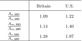
I start with changes in sectoral TFP for each region. Using the production function in the primary sector, the change in TFP in the primary sector of regionican be represented as

(Aa,i)1913

(Aa,i)1870

= (Ya,i)1913 (Ya,i)1870

(La,i)1870

(La,i)1913

αa

(Ni)1870

(Ni)1913

1−αa

(26)

The first term on the right hand side of (26) is obtained from Federico’s (2004) value-added index for Britain and the U.S.23 The second term, the change in labour force employed in primary sector, can be obtained from Broadberry and Irwin (2006). It only provides 1871 and 1911 figures for Britain and 1869 and 1909 figures for the U.S. Therefore I have to use the growth rates from Broadberry and Irwin to obtain the 1870 and 1913 values.24 _{Finally, the change in land endowment is taken from the} _Abstract

of British Historical Statistics for Britain and theCensus for the U.S.25

23

The index for Britain in 1870 is 107.2 and for the U.S. it is 38.8 with the 1913 levels for both countries normalized to 100.

24

For Britain’s annual growth rate of labour force in primary sector from 1861 to 1871 is about -1.2% and from 1901 to 1911 is about -0.08%. And for U.S. it is about 0.74% from 1859 to 1869 and 0.63% from 1899 to 1909.

(50)

Next I move on to manufacturing TFP. It is clear from the model that an

αmshare of revenue in manufacturing sector is distributed as labour income.

This implies the following equation

Ym,i =

wiLm,i

αmpm,i

(27)

I use equation (27) to derive an expression for TFP. To this aim I need the following equations derived from the model.

pm,i =

σm

1−σm

(Am,iα αm

m (1−αm)

1−αm₎−1_wαm

i G

1−αm

m,i (28)

Gm,i= 

 X

j

nj(pm,jTj,im)

1−σm 



1/(1−σm)

(29)

T_j,im =

nm,i

nm,j

₁₋1_σm

pm,i

pm,j

pm,jmij

pm,imii ₁₋1_σm

(30)

These equations are just restatements of equation (7), (2) and (A.1), respec-tively. Inserting (30) into (29), the price index can be expressed as

Gm,i =

nm,ip

1−σm

m,i X

−1

i ₁₋1_σm

(31)

where I defineXi = Ppmimii

jpmjmij as the home trade share (share of expenditure

on domestic products in total expenditure). Also from the model we know that nm,i = _α_m_pwiLmi

miF(σm−1) which can be plugged in (31). Then this can be

substituted in (28) which yields,

pm,i =wi h

A−1

m,i(Lm,iX

−1

i )

1−αm

1−σm

i₁₋1_αmσm−σm

(51)

In deriving (32) I dropped all the common parameters that will eventually cancel out when I calculate the change in TFP. I plug (32) into (27) to obtain,

Ym,i=

A1−σm m,i X

1−αm

i L

αm(1−σm)

m,i

₁₋_αmσm1

(33)

With (33), I can obtain the growth rate of TFP from 1870 to 1913 as

Am,1913

Am,1870

=

X1870

X1913

1−αm

1−σm _L_m,₁₈₇₀

Lm,1913

αm

Ym,1913

Ym,1870

1−αmσm

1−σm

(34)

where I dropped the regional subscript i. This approach of measuring the manufacturing TFP shock has the advantage that data on manufacturing intermediate usage does not have to be used as we do not have any accurate data on it anyway.26 Instead, the home trade share X can be calculated more accurately using trade and expenditure data.

To obtain Xus, I rely on The Historical Statistics of the United States.

It reports the ‘value of commodities destined for domestic consumption for 1869 to 1919’ (table Cd378-410). This corresponds to P

jpmjmij or total

expenditure and the value of imports is subtracted from this in order to obtain pm,usmusus or the expenditure on domestic products. As a result

Xus,1869 = 0.72 and Xus,1913 = 0.86.27 So the share of U.S. expenditure on

domestic manufacturing increased from 1869 to 1913.

I use Jefferys and Walters (1955) to calculateXb. They provide values for

‘consumption of home-manufactured consumer goods’ which corresponds to

pm,bmbb in the model. But they only include the value of final consumption

which means that expenditure on intermediate goods is not included. Their data are therefore rather limited for my purposes. The values for Xb,1870

and Xb,1913 are 0.865 and 0.714, respectively.

26