Original citation:
Drugov, Mikhail and Macchiavello, Rocco. (2014) Financing experimentation. American Economic Journal : Microeconomics , Volume 6 (Number 1). pp. 315-349.
Permanent WRAP url:
http://wrap.warwick.ac.uk/61952
Copyright and reuse:
The Warwick Research Archive Portal (WRAP) makes this work of researchers of the University of Warwick available open access under the following conditions. Copyright © and all moral rights to the version of the paper presented here belong to the individual author(s) and/or other copyright owners. To the extent reasonable and practicable the material made available in WRAP has been checked for eligibility before being made available.
Copies of full items can be used for personal research or study, educational, or not-for-profit purposes without prior permission or charge. Provided that the authors, title and full bibliographic details are credited, a hyperlink and/or URL is given for the original metadata page and the content is not changed in any way.
Publisher’s statement:
Permission to make digital or hard copies of part or all of American Economic
Association publications for personal or classroom use is granted without fee provided that copies are not distributed for profit or direct commercial advantage and that copies show this notice on the first page or initial screen of a display along with the full citation, including the name of the author. Copyrights for components of this work owned by others than AEA must be honored. Abstracting with credit is permitted.
http://dx.doi.org/10.1257/mic.6.1.315 A note on versions:
The version presented here may differ from the published version or, version of record, if you wish to cite this item you are advised to consult the publisher’s version. Please see the ‘permanent WRAP url’ above for details on accessing the published version and note that access may require a subscription.
Financing Experimentation
March 2013
Abstract
Entrepreneurs must experiment to learn how good they are at a new activity.
What happens when the experimentation is …nanced by a lender? Under common
scenarios, i.e., when there is the opportunity to learn by "starting small" or when
"no-compete" clauses cannot be enforced ex-post, we show that …nancing
experi-mentation can become harder precisely when it is more pro…table, i.e., for lower
values of the known-arm and for more optimistic priors. Endogenous collateral
requirements (like those frequently observed in micro-credit schemes) are shown to
be part of the optimal contract.
Keywords: Experimentation, Moral Hazard, Adverse Selection, Starting Small,
Competition.
“Each of us has much more hidden inside us than we have had a chance
to explore. Unless we create an environment that enables us to discover the
limits of our potential, we will never know what we have inside of us.”
Muhammad Yunus, Founder of Grameen Bank
1
Introduction
When people start a new activity, they might not know how pro…table it is, or how good
they will be doing it. They can only learn by trying it out. In other words, people must
experiment to learn about the activity or about themselves. An important example of
such a scenario is a person starting a business. This may be a poor woman in a slum
in India trying to open a small shop, or an IT-entrepreneur in Silicon Valley hoping to
found the next Google. In either case, if initial capital has to be borrowed, the lender –
be it a micro…nance institution in India or a venture capitalist in the US –…nances the
experimentation.
What happens when the experimentation is …nanced by a lender? The lender should
take into account that the borrower might misbehave, for example, by shirking or by
di-verting the loan; also, the borrower might (privately) acquire some information relevant
to the continuation of the project. In order to study such a setting, this paper builds a
simple model that embeds a two-period experimentation problem into a lending
relation-ship. The central insight of the paper is to show how, in the context of experimentation,
projects with higher net present value can be systematically harder to …nance.
A standard experimentation setting arises, broadly speaking, when certain activities
undertaken today generate valuable information that can be used in future decision
mak-ing.1 In its simplest form, standard experimentation involves, in at least two periods, a
choice between one activity with known returns (the so-called known arm), and another
activity with initially unknown returns (the so-called unknown arm). Experimentation
is then a particular form of investment: it involves a trade-o¤ between short-term costs
of generating information and long-term bene…ts of using it. Therefore, the higher the
discount factor, the lower the value of the activity with known returns and the more
optimistic is the prior belief about the unknown arm, the more the decision maker …nds
it attractive to experiment.
The paper studies a two-period model in which in each period an agent can start a
project. Initially, both the agent and the lender are uninformed about the e¤ort costs
needed to complete the project. Upon starting the project, the agent learns her e¤ort
costs. While it is optimal to complete the project regardless of the agent’s e¤ort costs
since the investment is already sunk, the agent might decide not to exert the e¤ort and to
divert the capital for private bene…t. In the second period the agent can obtain another
loan, depending on the …rst-period outcome and her communication with the lender.
Equipped with this simple benchmark, we study the resulting …nancing problem
un-der a number of plausible scenarios. First, we consiun-der the case in which the borrower
can experiment by “starting small”.2 We …nd that obtaining credit to …nance the
ex-perimentation might become harder precisely when experimenting is more valuable. By
experimenting, the borrower privately learns about herself and, therefore, in addition to
the standard moral hazard problem associated with borrowing, there is an adverse
se-lection dimension which emerges after the loan has been disbursed. The prospect of a
larger second-period project might make the selection of the right type of borrower more
di¢ cult since entrepreneurs have high incentives to fake short-term performance in order
to enjoy higher rents in the future. For the same reason, a lower payo¤ of the known
arm, i.e., the outside option, makes …nancing experimentation more di¢ cult. In other
words, the future rents which are helpful in solving the moral hazard problem (see, e.g.,
William P. Rogerson (1985) and Patrick Bolton & David S. Scharfstein (1990)) come at
the cost of rendering the adverse selection problem more severe.
Second, we consider the case in which the borrower can leave the relationship with the
original lender and seek …nance from alternative lenders in the second period. Motivated
by empirical evidence, we consider two di¤erent scenarios. First, we consider the case in
which “non-compete” clauses can be enforced, as in venture capital contracts (see, e.g.,
Steven N. Kaplan & Per Strömberg (2003)). Under this scenario, we show that the results
described above are completely robust to ex post competition. Second, we consider the
case in which “non-compete” clauses cannot be enforced, as is likely the case for bank
lending to SMEs (see, e.g., Vasso Ioannidou & Steven Ongena (2010)) or in microcredit
2A large body of work notes how …rms and relationships initially start small and then grow over time
lending in developing countries (see, e.g., Dean Karlan & Jonathan Morduch (2010)).
Under this scenario, we obtain a new result: …nancing experimentation can become harder
when initial priors about the pro…tability of the unknown arm are su¢ ciently optimistic.
This happens because a higher likelihood of successful experimentation allows an outside
lender to o¤er better contractual terms to the borrower once the initial sunk cost of
experimentation has been …nanced by the inside lender.
Finally, we explore the robustness of these results to the case in which the borrower
has access to a saving technology. The insight that experimentation can become harder
to …nance precisely when it is most valuable is robust to this extension. In addition, the
analysis also highlights how access to savings and ex post competition among lenders
interact to shape access to …nance.
The optimal contract in our model is similar to contracts typically o¤ered in practice.
The model highlights how retained earnings can be used to …nance payments which
induce the bad type of borrower to relinquish the project in the second period. This can
be achieved, for example, by using retained earnings to endogenously build up collateral.
The optimal contract, therefore, can mimic compulsory saving requirements (CSRs), a
common practice observed in microcredit that has, however, received little theoretical
attention.3 Similarly, in venture capital “purchase options” allocate to the investor the
right to acquire control over the project at a pre-speci…ed price. When the investor
exercises the option she e¤ectively pays an exit fee to the entrepreneur (see, e.g., Kaplan
& Strömberg (2003)). Besides rationalizing contractual features that appear to be used
in practice, the model yields a number of testable predictions on the relationship between
collateral, loan terms and project outcomes that are discussed in detail at the end of the
paper.
Related Literature
This paper belongs to a growing literature that combines experimentation and agency
problems. We apply our framework to a …nancing setting, which suggests to focus on a
di¤erent mix of agency problems and, more importantly, to consider several extensions,
e.g., scalability, competition, access to savings, which are usually left unexplored in the
3Under CSRs, a share of the repayment from earlier loan cycles is locked in into a saving account until
literature. As a result we derive a number of novel results, e.g., the non-monotonicity of
access to …nance with respect to the discount factor, the outside option and the prior.
Dirk Bergemann & Ulrich Hege (2005) consider an agent who can either explore an
in-novative project or shirk, in which case the project outcome (failure) is not informative.4
As in other dynamic contracting models without commitment (see, e.g., Jean-Jacques
La¤ont & Jean Tirole (1987)) they …nd that a higher discount factor can render
…nanc-ing more di¢ cult when the agent’s actions are observable. A key di¤erence with our paper
is that we assume the lender has full commitment power. In Gustavo Manso (2011) the
agent can experiment, shirk or exploit a known activity. He shows that motivating
exper-imentation requires dramatically di¤erent incentives from standard pay-for-performance
schemes, e.g., rewards for failure. Our application to …nancing suggests to consider
dif-ferent agency problems and focus on di¤erent comparative statics leading to the central
insight that projects with higher net present value can be systematically harder to
…-nance and implement. A contemporaneous paper by Matthieu Bouvard (2012) studies a
real-option model where a borrower experiments and the timing of …nancing is one of the
contractual variables. There, the borrower starts being better informed than the investor
about the probability of success while the costs of experimentation are exogenous. There
are no results about the e¤ects of the discount factor. Moreover, as mentioned above,
none of these papers considers ex post competition between lenders nor access to savings
by the agent.5
In Steven D. Levitt & Christopher M. Snyder (1997) and Roman Inderst & Holger M.
Mueller (2010) the principal also faces the combination of the moral hazard and interim
adverse selection where the project is terminated (or the agent is …red) following bad news
revealed by the agent. However, the mechanism at work there is di¤erent from ours. In
these two papers, the project outcome is a signal about the agent’s e¤ort and is used to
elicit the e¤ort. If the project is terminated, the outcome stays unknown and, therefore,
acting upon information ex post intervenes with the provision of incentives ex ante. In
our model, acting upon information obtained in the …rst period means deciding about the
second-period project which does not depend on the …rst-period e¤ort. Our mechanism is
4See also Dirk Bergemann & Ulrich Hege (1998) which is "a preliminary analysis of the same basic
model" (Bergemann & Hege (2005), p. 723).
5Other papers related to Bouvard (2012), such as Steven R. Grenadier & Andrey Malenko (2011) and
that the second-period moral hazard rent makes the interim information revelation more
costly. While the mechanisms are di¤erent, the interaction of moral hazard and adverse
selection is crucial in all three papers: each of them becomes trivial if only moral hazard
or adverse selection is present.6
The paper is also related to the literatures on the role of collateral (see, e.g., Helmut
Bester (1985) and David Besanko & Anjan V. Thakor (1987a)) and relational lending (see,
e.g., Steven A. Sharpe (1990) and Mitchell A. Petersen & Raghuram G. Rajan (1995))
in facilitating access to credit. There are, however, important di¤erences. The literature
on collateral has typically focused on the availability of exogenously given amounts of
collateral. In contrast, in our setting the value of collateral available in the second period
of the relationship to separate borrowers is endogenous. The relational lending literature,
instead, focuses on the e¤ects of ex post competition from outside lenders but ignores the
role of endogenous savings and collateral. In our setting, ex post competition from outside
lenders does a¤ect the ability to …nance the project despite the endogenous collateral that
can be created through savings.
The rest of the paper is organized as follows. Section 2 presents the model with a
unique project size. Section 3 introduces the extension with two project sizes and derives
the results on the e¤ects of the discount factor and the outside option. Section 4 studies
the e¤ects of competition and shows that a better agent, in the sense of lower expected
e¤ort costs, may …nd …nancing her project more di¢ cult. Section 5 explores robustness
of the results to savings. Section 6 …nds a realistic contract that replicates the direct
mechanism of Section 3, interprets micro…nance contracts in the light of our model and
discusses testable implications. Section 7 concludes. The proofs are in the Appendix.
6In Jacques Crémer & Fahad Khalil (1992) and Jacques Crémer, Fahad Khalil & Jean-Charles Rochet
2
The Model
2.1
Setup
There is an agent that lives for two periods, = 1; 2: In each period the agent has the
opportunity to undertake a project that needs an initial capital investment of1and yields return r when completed. A project that is not completed fails and yields0.
The agent has no assets and needs to borrow 1 unit of capital in order to start the project. She is protected by limited liability. The agent and lenders have a common
discount factor 2[0;1]across the two periods. The complete description of the timing of events and the contracts is postponed until Section 2.3.
To complete the project the agent needs to appropriately invest the unit of capital and
to exert e¤ort. The agent can divert a share 1 of the initial investment for private
consumption. If she does so, the project fails. The parameter re‡ects the di¢ culty for
the lender of monitoring the investment and transaction costs in diverting the investment.
There are two types of agent, good G and bad B; which remain constant over the
two periods. The cost of e¤ort for the good agent is eG = 0; and eB =e >0for the bad
agent.7 Initially, both the agent and the lenders are uninformed about the type of agent
and have a common prior about the probability of the agent being the good type. The
agent privately learns her type upon starting the project in period 1 but does not if she
doesn’t start the project. After having learned her type, she decides whether to exert
e¤ort and whether to divert the capital.
Whenever e¤ort is exerted and investment is not diverted, the project succeeds and
yields r; which is observable and veri…able. In any period in which the agent does not
undertake the project, she takes an outside option u >0. We make the following parametric assumptions:
Assumption 1 r 1< u+e:
Assumption 2 u < .
Assumption 3 maxf1; eg< r :
7The model can be also interpreted with the e¤ort cost being a characteristic of the project, rather
The …rst assumption implies that it is not optimal to invest if the agent is (known
to be) bad: the opportunity costs of investment 1 +u are higher than revenues r net of e¤ort costse:
The second assumption implies that the agent always prefers to start the project with
borrowed money rather than take her outside option u:
Finally, the third assumption has two implications. First, r 1> implies that the project generates enough revenues to solve the moral hazard problem of the good type.
Second,r > +eimplies that, once the project is started and the initial outlay of 1unit of capital is sunk, it is optimal to complete the project regardless of the agent’s type.
2.2
Optimal Experimentation by a Self-Financed Agent
Let us …rst consider the benchmark case in which the agent has enough wealth so that
she does not need to borrow. In this case the agent is the residual claimant of the project:
there are no incentive problems and, therefore, the …rst-best allocation is chosen.
Once she has started the project in period1, the agent exerts e¤ort and completes the
project regardless of her type (Assumption 3). In period2;she invests and completes the project again if she has learned that she is of the good type, since r 1> u. If she has
learned that she is of the bad type she prefers to take her outside option (Assumption
1):Conditional on having started the project in period 1, this is the …rst-best allocation.
Investment in period 1 can be thought of as experimentation: its costs are borne in period 1 while the bene…ts are realized in period 2: After the agent has learned her
type, she will be able to make an informed decision. The costs of experimentation are
given by the di¤erence between the opportunity costu and the expected surplus created
by the project in period 1, i.e., r 1 (1 )e: The bene…ts of experimentation are due to better decision-making in period 2: With probability ; the information gathered
through experimentation leads the agent to start a project, instead of taking the outside
option. With probability 1 , instead, the agent learns she is of the bad type and
takes her outside option. In this case, the information gathered through experimentation
does not change her decision.8 The value of information therefore equals (r 1 u):
Experimentation is optimal if its costs are lower than its bene…ts.
8The agent is considering whether to experiment or not in period 1. If she decides to not experiment
Contracts offered & selected
Alearns type & reports it
t Adecides
on effort & diversion
Period 1 Period 2
Investment takes place Project outcome
is realized and transfers made Investment
takes place
Adecides on effort & diversion
[image:10.595.83.516.76.146.2]Project outcome is realized and transfers made
Figure 1: Timing of events
Lemma 1 If the agent does not need to borrow, experimentation (investment in period
1) is optimal if and only if E; where
E
u+e(1 ) (r 1)
(r 1 u) : (1)
As in standard experimentation models, starting the project in period 1 becomes pro…table if is high enough, if the agent is su¢ ciently con…dent about being of the good
type (high ), if the value of the known activity is not too high (lowu) and if the project
yields high returns (high r 1).
2.3
Contracts and Timing of Events
We now describe contracts and the structure of the credit market. Lenders compete in
the market and make zero pro…ts in expectation.9 They have full commitment power
and o¤er two-period contracts. The project is …nanced in period 1. For simplicity, we initially assume that i) the agent cannot change her lender in period 2 (but she can
take her outside option u), ii) the agent cannot save on her own. We relax these two
assumptions in Section 4 and Section 5.
The timing of events is the following. Immediately after the agent learns her type,
she sends message m 2 fG; Bg to the lender.10 According to the message, the contract
speci…es the agent’s actions in period 1; a transfer conditional on the project outcome in period 1 and a re-…nancing policy in period 2. The contract also speci…es a transfer
in period 2 conditional on project outcomes in periods 1 and 2: The timing of events is summarized in Figure 1.
9The main insights of the paper are preserved if the contract maximizes lender’s pro…ts subject to
the borrower incentive and participation constraints. See the discussion at the end of Section 2.5.
10Since lenders have commitment power and contracts are exclusive, the Revelation Principle applies
We say that an allocation can be …nanced if there exists a contract that gives
appro-priate incentives to the agent and satis…es the lender’s zero-pro…t constraint. In the next
Section we analyze when a lender can …nance the …rst-best allocation described above.
In Section 2.5 we show which allocation is …nanced if the …rst best is not possible.
2.4
Financing the First Best
In this Section we study when the …rst-best allocation, that is, the one chosen by a
self-…nanced agent, is …nanced. To do so, we proceed in two steps. First, we …nd the
cost-minimizing contract, that is, the contract that …nances the …rst best with the least
possible transfers. Second, we …nd for which parameter values this contract allows the
lender to earn non-negative pro…ts.
To …nd the cost-minimizing contract we need to consider all the relevant incentive
compatibility, truth-telling and limited liability constraints for the two types.11
Remem-ber that in the …rst-best allocation only the good type is re…nanced in period2 but both types must complete the project in period 1: The following constraints, therefore, need
to be satis…ed. First, the good type must prefer to complete the project in both period
1 and period 2: Second, the bad type must prefer to complete the project in period 1.
Third, both types must have an incentive to reveal their type truthfully. Finally, the
contract must satisfy all relevant limited liability constraints.
We …rst prove the following Lemma.
Lemma 2 The net present value of the required minimum transfers to the good and bad
types to implement the …rst best is given by
TG= +e+ u and TB = +e; (2)
respectively.
Proof. See Appendix.
In period1, the project should be completed independently of the type of agent since,
at that stage, the initial outlay of 1 unit of capital is sunk (Assumption 3). Since the bad type is not given a project in period 2; the contract must give a transfer worth at
11To keep exposition simple and avoid too much notation in the main text, we relegate to the Appendix
least +eto compensate for not stealing and for her e¤ort cost. This, however, gives an
incentive to the good type to pretend to be the bad type. Hence a minimum transfer of
+e; with an additional compensation for not taking the project in period 2; must be
paid to the good type as well.
Are those transfers su¢ cient to satisfy the other constraints? It turns out they are.
In principle, the good type also needs to be given incentives to complete the project in
period 2: The minimum amount of rents necessary to induce the good type to complete
the project in period2 is equal to : However, 1implies that these rents are smaller than those required to induce the bad type to complete the project in period 1: Since
rents to the good type can be paid in period 2; a contract that induces the good type to reveal her type truthfully pays su¢ cient rents to ensure the project in period 2 is
completed.12 Conversely, the bad type does not want to pretend to be the good type and
try to get a project in period2:
The …rst best can be …nanced when the project revenues are large enough to pay the
cost-minimizing transfers characterized in Lemma 2, i.e., when
(r 1) (1 + ) TG+ (1 )TB:
This expression can be rewritten as
F B +e (r 1)
(r 1 u) : (3)
This leads to the following proposition.
Proposition 1 The …rst-best allocation is …nanced if and only if F B.
Threshold F B is higher than the one of the self-…nancing agent, E in (1). Incentive
problems create rents that make experimentation more expensive but do not change
the nature of the problem. Comparative statics on F B are similar to the one on E:
experimentation is more likely to be …nanced for more optimistic priors ;higher discount
factor ; higher project pro…ts r 1 and for lower values of the outside option u, e¤ort
costs e and the share of funds that can be diverted, .
12This is similar to the "reusability of punishments" introduced by Dilip Abreu, Paul Milgrom & David
2.5
Financing the Second Best
The …rst-best allocation cannot be …nanced for every con…guration of parameters in which
experimentation is pro…table. The reason is that inducing the bad type to complete the
…rst-period project requires paying informational rents to the good type as well, and this
might be too costly if the bad type is very unlikely. The borrower and the lender may
then agree on a contract that let the bad type fail in period 1 and …nances the project
in period 2 conditional on the successful completion of the project in period 1: In other words, as in standard adverse selection models, the lender may shut down the bad type
if its probability is low enough. The contract then only needs to solve the moral hazard
problem of the good type. This is the second-best allocation.13
The good type has to be incentivized to complete the project in period 1; which requires a transfer worth at least + u: Since 1; these rents are su¢ cient to also
ensure that the good type completes the project in period 2; which requires a transfer worth : The bad type, on the other hand, does not require any transfer since she does
not complete the project in period 1and then takes her outside option in period 2:
The second best, therefore, can be …nanced when the project revenues are larger than
the transfers required to induce the good type to repay in both periods, i.e.,
r 1 + (r 1) ( + u):
This expression can be rewritten as
SB 1 (r )
(r 1 u). (4)
The comparative statics follows the standard logic: a higher ; a higher and a lower
u expand the region in which the second best can be …nanced. The next proposition
characterizes the region where the second best is …nanced and Figure 2 illustrates it.
13The contract could implement the allocation in which the bad type receives a project in the second
Proposition 2 The second-best allocation is …nanced if and only if
SB
< F B:
Proof. See Appendix.
A monopolistic lender which maximizes pro…ts subject to the agent participation and
incentive compatibility constraints trades o¤ e¢ ciency and rents. In particular, for
and such that = F B and > SB the lender’s pro…ts from …nancing the …rst-best allocation are zero (by construction) while …nancing the second-best allocation yields
positive pro…ts. A monopolistic lender then chooses the second-best allocation. The
region where the …rst-best allocation is …nanced shrinks while the one of the
second-best allocation expands. However, comparative statics with respect to ; and u are
qualitatively preserved.
3
Starting Small
In many contexts, an agent might decide to experiment by “starting small” and then
later to scale up the project if she learns that the activity is pro…table. In our context,
“starting small” has the additional advantage that it might reduce the informational
rents that must be paid to the agent to reveal her type and exert e¤ort. In this Section
we show that allowing the agent to “start small” generates novel implications that are
qualitatively di¤erent from the results obtained in the previous Section: experimentation
might become harder to …nance when it is more pro…table.
We now assume that a small project is also available. The small project is a
propor-tionally scaled down version of the project studied above (that we will call a large project
for clarity). Speci…cally, the small project yields revenues r; costs an initial investment
equal to (and so can be diverted) and requires e¤ort costs e from the bad type.
Starting the small project still perfectly reveals the agent’s type.
As a benchmark, consider a self-…nanced agent.
Lemma 3 A self-…nanced agent never implements the small project.
Proof. See Appendix.
Assumption 4 ( u+e) < < (ru1):
The assumption < (ru1) implies that a small project isper se unpro…table: the only
reason to undertake a small project is to learn the type of the agent. The assumption,
therefore, rules out cases in which the small project is …nanced in both periods. The
assumption > ( u+e) ensures the agent’s participation in the project.
Assumption 4 implies that we can restrict attention to four allocations. Two
alloca-tions we considered above in which a large project is …nanced in period 1, that is, the …rst best of Section 2.4 and the second best of Section 2.5. Two new allocations are the
ones in which a small project is …nanced in period 1and is either completed or not, and the large project is …nanced in period 2 is the agent is of the good type. For clarity, we
refer to those allocations as …rst best when starting small and second best when starting
small.14
Let us …nd out the conditions under which …nancing the …rst best when starting
small is possible. As in Section 2.4, we again proceed in two steps. First, we …nd the
contract that …nances the allocation with the least possible transfers. This is the next
Lemma. Second, we …nd for which parameter values this contract allows the lender to
earn non-negative pro…ts.
Lemma 4 De…ne = u+e. The net present value of the required minimum transfers to the good and bad types to implement the …rst best when starting small is given by
8 < :
TS
G = ( +e) + u TS
B = ( +e)
; if and
8 < :
TS G = TS
B = ( u)
;if > . (5)
Proof. See Appendix.
The small project of period1should be completed independently of the type of agent.
Since the bad type is not given a project in period 2; the contract must give a transfer worth at least ( +e) to compensate for not stealing and for her e¤ort cost. This gives
an incentive to the good type to pretend to be the bad type.
In contrast to the case in which the project has the same size in both periods, however,
these transfers may not be su¢ cient to satisfy other constraints. If > ( +e) + u;
14Analogously to fn. 13 above, it is easy to show that the bad type is never given a small project
the bad type is tempted to pretend to be the good type; get a project in period 2
and to run with the money. Which constraint binds, therefore, depends on whether
? ( +e) + u; i.e., ? ; as described in Lemma 4. Note that this inequality can be rewritten as ? u+e: It is then clear that there is a one-to-one correspondence
between the discount factor and scale ; i.e., what matters is the weight, in present
value terms, of the …rst-period rent relative to the second-period rent.
If u+e the …rst-period rents determine the costs of implementing any given
allocation and, therefore, the analysis proceeds as in Section 2 with the …rst-period project
rescaled by factor : If, instead, < u+e the analysis might change. In the reminder of
the paper, we focus on this case.
Assumption 5 < u+e.15
The …rst best when starting small can be …nanced when the project revenues are
large enough to pay the cost-minimizing transfers characterized in Lemma 4, that is,
(r 1) ( + ) TS
G + (1 )TBS. If ; this expression can be rewritten as
F B S
+e (r 1)
(r 1 u) : (6)
If > , this expression can be rewritten as
F B S
8 < :
r 1
(1 )( u) (r 1 ) if
( u) (r 1) r 1 u
1 otherwise
: (7)
This leads to the following proposition. De…ne
= 1 r 1 +e
u
r 1 u; (8)
so the curves F BS and F BS intersect at( ; ).
Proposition 3 (i) First best when starting small can be …nanced if and only if F BS
F B S .
(ii) There is a region where the …rst best when starting small is …nanced. In particular,
it is …nanced at ( ; ).
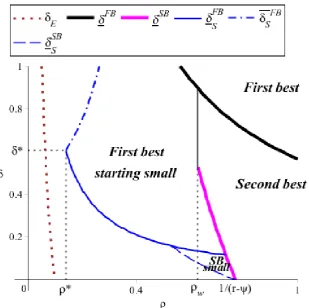
Figure 2: Financed allocations for r = 1:7; u= 0:15; = 0:4; e= 0:61 and = 0:15. At
w =
1+ (r 1 e)
r e the welfare in the second best allocation equals the one in the …rst best
when starting small.
Proof. See Appendix.
For the proof of part (ii) we show that at( ; )neither the …rst-best nor the
second-best allocations in which the large project is …nanced in period 1 are possible. In Figure
2 we draw a numerical example showing where each allocation is …nanced.16
Constraint (6) is very similar to (1) and (3): for low enough the pro…ts earned
in period 2 can be used to …nance the agent’s rent that must be paid to complete the
project. When is su¢ ciently high, however, the bad type is tempted to “take the money
and run” in period 2, that is, the truth-telling constraint of the bad type may become
binding. In period2, the lender needs to pay uto prevent the bad type from obtaining a project. The lender faces a de…cit of (1 ) ( u) (r 1 ) which has to be
…nanced by the …rst-period pro…ts (r 1). A higher ; therefore, reduces the value of period 1 pro…ts relative to the second-period de…cit and makes it harder to …nance
16For completeness, we derive in the Appendix the region where the second best when starting small
experimentation. Thus, the direction of (7), that has to be below a certain threshold,
is the opposite to the direction of (1), (3) and (6).17
While it is generally perceived that future rents associated with a project are helpful
to solve moral hazard (see, e.g., Rogerson (1985) and Bolton & Scharfstein (1990)),
this paper shows that under initial uncertainty about these rents, they might attract
undesirable borrowers and, therefore, lower the ex ante borrowing capacity. Interestingly,
these rents are increasing in the net present value of the project, implying that more
pro…table projects might be harder to …nance.
The logic is illustrated by the comparative statics with respect to the discount factor
;the outside optionuand the scale :If ;a higher expands the interval of values
of for which the …rst best when starting small can be …nanced. If > , a higher
shrinks this interval. Similarly, the comparative statics with respect to the outside option
u is non-monotonic. When , a higher u reduces the costs of being denied access
to credit in period 2. This shifts F BS upwards (see (6)) and, hence, shrinks the region in
which …nancing the …rst best when starting small is possible. When > , a higher u
reduces the rent needed to keep the bad type out in period 2. This shifts F BS upwards
(see 7)) and expands the region where …nancing the …rst best when starting small is
possible. Thus, in contrast to the case of a self-…nanced agent (1) and the …rst best (3),
a higher outside option makes lending easier. Analogously, a lower facilitates …nancing
for (see (6)) and hampers it for > (see (7)). The latter point implies that
the agency problem puts a lower bound on the downsizing of the experimentation round.
The remaining comparative statics, however, have the expected sign.
We then summarize the discussion by its corollary.
Corollary 1 There exists a region in the space ( ; ) where the …rst best when starting
small is …nanced and which shrinks with a loweru and where a higher requires a higher
. In that region, a higher value of experimentation makes …nancing it more di¢ cult.
17A useful analogy is dynamic adverse selection models without commitment (see, e.g., La¤ont &
4
Ex Post Competition
In Section 2 we have considered the case in which the borrower cannot seek …nance from
outside lenders in period 2. This Section relaxes this assumption. The Section has two
goals: i) check the robustness of the main result in Section 3 to the presence of ex post
competition, and ii) derive additional results on the relationship between competition,
value of the project, and …nancing constraints.
We follow the relational lending literature (see, e.g., Sharpe (1990)) and assume that
outside lenders do not observe the communication between the inside lender and the
borrower but can observe the …rst-period outcome of the project. We then consider two
di¤erent scenarios, depending on whether the original lender can enforce loan contracts
that are contingent on whether the borrower takes outside …nance from an alternative
lender (for simplicity, contingent contract case) or not (noncontingent contract case).
Both scenarios are likely to be relevant depending on the context. For example, J.B.
Bar-ney, Lowell Busenitz, Jim Fiet & Doug Moesel (1994) and Kaplan & Strömberg (2003)
…nd that venture capital contracts commonly include “non-compete”and “vesting
provi-sion” clauses that make it harder for the entrepreneur to hold-up the venture capitalist.
In other contexts, however, lenders do not have the ability to condition the terms of
their relationship with borrowers on whether borrowers access other sources of …nance
following the termination of their relationship. An example of such a circumstance is
(micro)credit to small, typically informal, microenterprises in developing countries (see,
e.g., Craig McIntosh & Bruce Wydick (2005) and Karlan & Morduch (2010) for a
discus-sion). Even in countries with developed …nancial systems, the type of hold-up we consider
prominently features in discussions of bank …nance to SMEs (see, e.g., Dietmar Harho¤
& Timm Körting (1998), Allen N. Berger & Gregory F. Udell (2006) and Ioannidou &
Ongena (2010)).
The exact e¤ects of competition depend on the contracts that the inside lender can
o¤er. With contingent contracts the inside lender counteracts outside lenders’ o¤ers
successfully and, therefore, competition in period 2 has no e¤ect (Proposition 4) on the results. With noncontingent contracts, instead, competition qualitatively changes the
results. In particular, the …rst-best allocation cannot be …nanced at all. Moreover, a
higher probability of the good type, , may have a negative e¤ect on the possibility to
con…rms the main …nding in Section 3 that …nancing experimentation might become
harder precisely when it is most valuable.
Preliminary Observations and Robustness of the Result in Section 3
In the …rst best both types complete the project in period 1 and, therefore, outside lenders do not know the type of the agent that applies to them. As outside lenders have
one-period relationship with the agent, they cannot …nance the small project (Assumption
4) and they have to let the bad type fail (Assumption 2 and 3). Then, they prefer to pay
u to the agent who reports to be of the bad type rather than …nance the project that
costs one (this can be done, e.g., by giving a small loan). Thus, outside lenders free ride
on the information generated by the inside lender.
Competition between outside lenders makes them pay the highest possible rent to the
good type driving their pro…ts to zero. The inside lender, however, always structures
a contract that gives incentives to the bad type to seek funds from outside lenders as
this makes it harder for outside lenders to compete. The highest rent outside lenders
can pay to good type while still breaking even in expected terms is therefore given by
r 1 1 ( u). This rent has to be above for the agent to complete the project, i.e.,
> comp u
r 1 u (9)
is necessary for the outside lenders to be able to o¤er loans in period 2. For comp outside lenders are unable to attract the good type without making losses. When this is
the case, the conditions for implementing all the allocations are the same as in Sections
2 and 3. Since , de…ned in (8), is smaller than comp, there always exists a region where
the …rst-best when starting small is …nanced and where the comparative statics are as
described in Corollary 1.
Corollary 2 There exists a region in which the comparative statics described in Corollary
1 holds when there is ex-post competition from outside lenders.
4.1
Competition with Contingent Contracts
We begin by considering the case in which the lender can o¤er contracts that are
contin-gent on whether the borrower completes, fails, or does not take up a project …nanced by
Proposition 4 When the inside lender can write contingent contracts, ex post
competi-tion does not bite. The regions in which each allocacompeti-tion can be …nanced are as
character-ized in Propositions 1, 2, 3 and 8.
Proposition 4 can be easily proven by construction. In particular, consider any
con-tract that implements the desired allocation in the absence of ex post competition. To
respond to ex post competition, the inside lender has to include in that contract the
fol-lowing “vesting provision”: the borrower has the option to purchase the right to continue
the project in period 2 at a priceF. To exercise the option, the borrower needs to borrow
1 +F from the outside lender. A priceF > r 1 is su¢ cient to ensure that there does not exist a contract in which i) the borrower obtains su¢ cient funds, invests and repays
the loan, and ii) the outside lender makes non-negative pro…ts (see Philippe Aghion &
Patrick Bolton (1987) for a similar logic).
4.2
Competition with Noncontingent Contracts
We now consider the case in which the lender cannot write contracts contingent on what
the borrower does upon leaving the relationship in period2. We focus on the case when
> comp, i.e., when competition from outside lenders is possible.
Proposition 5 Under competition from outside lenders with noncontingent contracts:
(i) the …rst best cannot be …nanced,
(ii) the …rst best when starting small can be …nanced if comp (1+e)(( ur 1))
r 1 ( u)
comp
,
(iii) the region in which the second best can be …nanced is as in Proposition 2.18
Proof. See Appendix.
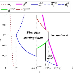
Figure 3 illustrates the Proposition through an example. Proposition 5 contains two
main results. First, the …rst best is impossible to …nance (part (i)). This happens
because the second-period pro…ts of the inside lender, which are limited by competition to
(1 ) ( u), are not su¢ cient to compensate for his …rst-period loss of +e (r 1).
More importantly, Proposition 5 shows that a higher is detrimental to the …nancing
of experimentation (part (ii)). Since comp increases in while comp decreases in , a
18For completeness, we also show that the region in which the second best when starting small can be
Figure 3: Financed allocations under competition with noncontingent contracts for r = 1:7; u = 0:15; = 0:4; e = 0:61 and = 0:15. At w = 1+ (rr 1e e) the welfare in the second-best allocation equals the one in the …rst best when starting small.
higher makes …nancing the …rst best when starting small more di¢ cult. A higher
might make the …rst best when starting small impossible to …nance while no other
allocation can be …nanced either. The intuition for these results is that outside lenders
“bite the hand that feeds them”. Attracting the good type, they increase the inside
lender’s costs. A higher allows outside lenders pay a higher rent to the good type
to a point that cannot be matched by the inside lender, who also bears the costs of
experimentation. But without the information generated by the …rst period …nancing,
outside lenders cannot survive for some intermediate values of and, therefore, the market
completely shuts down.
Finally, if outside lenders believe that only bad types do not complete period1projects
(second-best allocations), the good type can no longer pretend to be the bad type without
loosing access to outside lenders in period2. The bad type does not get any transfer and
all transfers to the good type can be paid upon successful completion of both projects.
competition or not, then, simply depends on whether the rent paid by outside lenders to
the good type in period 2, i.e., (r 1); is larger than the rent necessary to have the project completed in both period under no competition: In the second best, it turns out
it is not: the inside lender is in any case paying high rents to complete a large project in
period 1.
5
Savings
This Section shows that the main results derived in Section 3 and Section 4 are robust if
the borrower can (partially) self-…nance the period2project through endogenous savings
acquired in period 1.
The good type, in particular, may prefer to divert in period 1, self-…nance the
project in period2 and obtain returns r 1. If diverting in period1 is not enough to self-…nance the project in period 2, the agent may apply to outside lenders when they
are available. For simplicity, we assume a costless saving technology for the agent. The
agent earns an interest rate1 +i= 1 on her private savings: if the agent savess in period
1 her savings are worths(1 +i) = s in period 2.
We …rst study the case when there are no outside lenders. When a large project is
…nanced in period 1, self-…nancing is then possible if 1. With the small project …nanced in period 1, the condition is 1. The next proposition shows that the
possibility to save and self-…nance in period2does not matter in the …rst-best allocations but does matter in the second-best allocations.
Proposition 6 When the agent can save on her own and there are no outside lenders,
(i) The regions where the …rst best and the …rst best when starting small can be …nanced
are as characterized in Section 3,
(ii) The second best cannot be …nanced for and < r 1 ; the second best when
starting small cannot be …nanced if and < 1 r .
19
Proof. See Appendix.
When the agent completes the project in period1she gets a high rent that makes her prefer to stay with the lender rather than divert the …rst-period funding and self-…nance.
19Otherwise, the second best can be …nanced as characterized in Proposition 2 and the second best
Consider the …rst best when starting small. The good type gets at least ( +e) +
u when staying with the lender if both projects are successful. Diverting and
self-…nancing she gets + (r 1): The condition (which is necessary for
self-…nance to be possible) then implies that the value of self-self-…nance is always smaller than
the rents obtained by completing the project. The same argument applies for the …rst
best (replacing by1).
In the second-best allocations, in contrast, the agent gets a smaller rent since she does
not complete the …rst project. Getting + (r 1)(or + (r 1)) by self-…nancing is better than the minimum transfer + u (or + u). Thus, the lender has to increase
her transfer and the possibility of savings shrinks the region in which the second-best
allocations can be …nanced.20
We now turn to the case in which the agent can save and there are outside lenders
from whom she might borrow if her savings are not enough to …nance the project. We
characterize when the …rst-best allocations can be …nanced focusing on the case of
non-contingent contracts.
Proposition 7 When the agent can save and borrow from outside lenders under
non-contingent contracts,
(i) the …rst best cannot be …nanced,
(ii) the …rst best when starting small cannot be …nanced if u. For > u,
there exist thresholds compsav > comp; compsav < comp and comp
sav < comp such that: a] if comp
sav the characterization in Proposition 3 applies, and b] if > compsav the …rst best
when starting small can be …nanced if compsav compsav .21
Proof. See Appendix.
The main message of Proposition 7 is that the borrower’s ability to save and borrow
from outside lenders interact to make lending even more di¢ cult. The interaction stems
from the fact that outside lenders can separate types at a lower cost. In particular, the
constraint that the rent of the good type has to be at least can be satis…ed more easily
since outside lenders invest less into the project and pay less to the bad type.
20In our model the possibility to save and self-…nance only makes …nancing experimentation harder.
The reason is that …nancing decision in period 2 is always e¢ cient. In the models built on Bolton & Scharfstein (1990), where ine¢ cient termination is used in the equilibrium, saving and self-…nancing has an e¢ ciency bene…t allowing the agent to continue when the lender would terminate as, for example, in Roman Inderst & Holger M. Mueller (2003).
If the agent can save more than ( u); outside lenders can separate types at no
cost since the bad type does not try to obtain funds from outside lenders and to divert
in period 2:Only the good type then applies for the loan and gets all the project rent
r 1. If the inside lender matches this rent to keep the good type, he does not make any pro…t in period 2. When the agent cannot save that much, the bad type also wants
to apply for the loan from outside lenders and the analysis is then similar to the one
of competition without savings as in Section 4.1. In particular, a higher still makes
…nancing the …rst best when starting small more di¢ cult (i.e., compsav increases with
while compsav decreases with ).
We summarize this discussion noting
Corollary 3 The results in Section 3 and Section 4 are qualitatively robust to the case
in which the borrower has access to a saving technology. In particular, there always exist
regions in the space ( ; ) where 1.] the …rst best when starting small is …nanced and which shrinks with a lower u and where a higher requires a higher ; 2.] a higher
makes …nancing impossible. In these regions, a higher value of experimentation makes
…nancing it more di¢ cult.
6
Indirect Mechanism
We have investigated so far which allocations, if any, can be …nanced. It is important,
however, to know whether there are realistic contracts that replicate the direct mechanism
that implements a given allocation and to derive testable implications. This section
answers both questions. We consider only the …rst best when starting small as in Section
3 to keep the paper at a reasonable length.
Due to the agent’s risk-neutrality, the structure of payments in the optimal contract
is not uniquely determined. To choose a particular contract, we impose a “minimum
consumption spread” re…nement. Among all the contracts that implement the …rst best
when starting small, we focus on those that minimize i) the di¤erence in the net present
value of consumption across types, and ii) the di¤erence in consumption across periods
for each type.22
22Essentially, we assume that the agent has a utility function which is concave in consumption and
separable in e¤ort and consumption, i.e., U(c) e; with U0( )> 0 and U00( )< 0, and then take the
Denote by ci; i=G; B; = 1;2; the consumption of type i in period . We proceed
in three steps. First, we derive the net present value of consumption given to each type.
Second, we derive the consumption allocation to each type in each period taking into
account necessary incentive constraints. Finally, we describe a contract that induces the
resulting consumption allocation.
Denote by the di¤erence between the expected project revenues of the relationship
and the minimum transfers necessary to implement the …rst best when starting small,TS G
and TS
B (characterized in Lemma 4):
= ( + ) (r 1) TGS+ (1 )TBS .
The project can be …nanced if 0: Remember that TGS =TBS+ u:We can rewrite
= ( + ) (r 1) + (1 ) u TGS:
SinceTS
G >(1 + )u;it follows that, if the project can be …nanced, the lender can design a
contract in which the constraint cB
2 u (which would stem from the non-transferability
of u) never bites. Transferable revenues, ( + ) (r 1); and non-transferable
pay-o¤s,(1 ) u; generated by the relationship can be aggregated and competition among lenders ensures that the net present value of consumption for each type is equal to
C( ) = ( + ) (r 1) + (1 )u.23
Contracts satisfying the “minimum consumption spread” re…nement implement the
following consumption allocation:
1. Perfect consumption smoothing across types, cB
1 + cB2 =c1G+ cG2 =C( );
2. Perfect consumption smoothing across periods for the bad type,cB1 =cB2 = C1+( ) > u;
3. Perfect consumption smoothing for the good typecG
1 =cG2 = C( )
1+ ifC( ) (1+ ) :
Otherwise, cG1 =C( ) < cG2 = :
The optimal contract provides full consumption insurance to the borrower against bad
realizations of her entrepreneurial talent. The contract also provides perfect consumption
smoothing across the two periods for the bad type since, conditional on completing the
23We derive testable predictions by considering correlation patterns driven by heterogeneity in across
project in period 1, no further constraint must be satis…ed. Furthermore, in each period
the bad type consumes more than her outside option u: The contract, however, might
fail to achieve perfect consumption smoothing for the good type. Indeed, since the good
type has to obtain at least in period 2 to complete the project, perfect consumption smoothing is possible only if can also be paid in period1, i.e., if C( ) (1 + ) :
An Optimal Contract: Application to Micro…nance
Is there an indirect mechanism that implements the consumption allocation described
above and resembles a real world contract? As an example, consider the contract C
fd1; d2; sC; ig de…ned as follows. The agent borrows in the beginning of period 1. If
the project yields revenue r, the agent repays d1 at the end of period 1. The borrower
can apply and obtain funding in period 2 under two conditions: i) she has repaid period
1 loan, and ii) she posts collateral at least equal tosC: If the borrower seeks and obtains
funding in period 2; she borrows one unit of capital and repays d2 if the project yields
revenuer. Otherwise, she defaults and loses the posted collateral. Finally,iis the interest
rate paid by the lender on the saving account held by the borrower.
Denote bysBand sG the saving chosen by the bad type and good type. Consumption
patterns are then de…ned by
cG1 = r d1 sG and cB1 = r d1 sB in period 1, and (10)
cG2 = r d2+ (1 +i)sG and cB2 = (1 +i)s B
+uin period 2
As in Section 5, let us set, with no loss of generality,(1 +i) = 1:The remaining terms
of the contract can be computed substituting the appropriate consumption values in (10).
In period 2 the bad type consumes more than the income she derives from taking the
outside option, cB2 = C1+( ) > u: The consumption in excess of income in period 2 gives a positive saving balancesB( ) = C( )
1+ u :Substituting intoc B 1 =
C( )
1+ ;the amount to
be repaid to the lender is equal tod1( ) = r C( ) + u;which is decreasing in :24 The
model implies that better borrowers consume (and save) more and receive better terms
on the period1 loan.
Substituting d1( ) and the appropriate consumption values in (10), we …nd sG( ) =
24The described contract is feasible if d
1( ) 0; i.e.;if (r 1 u):The condition is veri…ed,
maxf ( u); sB( )
g: In turn, this impliesd2 =r u:WhenC( )<(1 + ) ;the good
type consumes less and saves more than the bad type in period 1.
Note thatsB( )and sG( )are not part of the contract with the lender. Given sB( )
and a requested collateral sC; the bad type does not apply for a loan in period 2 (on
which she would default) if
+ s
B( ) sC
C( ) 1 + ;
i.e., ifsC ( u). We saw this condition in Section 5 (see discussion after Proposition
7) under which outside lenders can separate the types at no cost.
When C( ) (1 + ) ; both types optimally save more than sC but only the good
type applies for a loan. When C( ) < (1 + ) ; however, the bad type saves less than
sC: The good type, instead, is required to save sC = ( u) to obtain the loan. The
optimal contract, therefore, requires the borrower to save a larger amount in order to
continue borrowing in period2:
The contract uses retained earnings to endogenously build up collateral and screen
out the bad type. One way in which this can be achieved, is through compulsory saving
requirements (CSRs). An example of a loan contract with compulsory saving
require-ments is found in micro…nance, broadly de…ned as the provision of small uncollateralized
loans to poor borrowers in developing countries. CSRs are a common feature of
mi-crocredit schemes (whenever the regulatory framework allows MFIs to collect deposits).
For instance, the three largest micro…nance institutions in Bangladesh (Grameen Bank,
BRAC and ASA) have been collecting compulsory regular savings from their clients from
the very start of their programs (see, e.g., Asif Dowla & Dewan Alamgir (2003)). All of
the …ve major micro…nance institutions described by Morduch (1999) use combinations
of borrowing and saving. In recent years, many MFIs have also started o¤ering more
‡exible savings products (see, e.g., Nava Ashraf, Dean Karlan, Nathalie Gons & Wesley
Yin (2003)). CSRs are payments that are required for participation in the scheme, are
part of loan terms, and are required in place of collateral. The amount, timing, and
access to these deposits are determined by the policies of the institution rather than by
the clients who are typically allowed to withdraw at the end of the loan term, after a
When the second-best allocation is …nanced, CSRs are never needed. Indeed, the bad
type reveals herself by defaulting in period1. Therefore, the model implies that CSRs are more likely to be observed when the contract induces all borrowers to repay their loans.
This suggests a connection between extremely high repayment rates and the prevalent
use of CSRs observed in micro…nance, as informally discussed in Morduch (1999).25
Empirical Predictions on the Use of Collateral
Besides rationalizing contractual features used in practice, the model yields a number
of testable predictions on the relationship between collateral, loan terms and project
outcomes. Many models predict that lower risk borrowers pledge more collateral (see,
e.g., Besanko & Thakor (1987a), David Besanko & Anjan V. Thakor (1987b), Yuk-Shee
Chan & Anjan V. Thakor (1987) and Yuk-Shee Chan & George Kanatas (1985)). This
observation appears to be at odds with lending practices that associate the use of collateral
with riskier borrowers (see, e.g., Kose John, Anthony W. Lynch & Manju Puri (2003)).
In the model, the good type obtains the loan in period2and is required to post collateral worth sC = ( u): Since the bad type never obtains a loan in period 2, the model
impliesno relationship between amount of collateral and risk in a cross-section of period
2 borrowers.
Suppose the borrower has some wealth at time zero which can be posted, at some small
variable cost, as collateral. This extension of the model does imply the observed
empir-ical relationship between collateral and risk. If the borrower is credit constrained (i.e.,
cannot …nance the …rst-best allocation) she would post the minimum collateral necessary
to obtain the loan. Since …nancing requirements are given while the surplus available is
increasing in , borrowers with lower post higher collateral to obtain funds. In other
words, in a cross-section of borrowers, the model predicts a positive relationship between
collateral posted and likelihood of termination (if a …rst-best type allocation is
imple-mented) or likelihood of default (if a second-best type of allocation is impleimple-mented).26
25The model can be applied to other contexts besides microcredit contracts. For example, the payment
to the (bad type of) borrower to make her relinquish the project can be interpreted as shift of the control from the entrepreneur to the investor in venture capital …nance. This can be implemented through a “purchase option”: when the investor exercises this option he e¤ectively pays an exit fee to the entrepreneur (see, e.g., Kaplan & Strömberg (2003)).
26As in standard models of moral hazard or adverse selection in credit market (see, e.g., Dean Karlan
7
Conclusion
Exploration of unknown activities lies at the heart of this model. What happens when
such activities are …nanced by a lender? The paper has shown that introducing agency
problems changes the nature of experimentation. In particular, we have shown how, in the
context of experimentation, projects with higher net present value can be systematically
harder to …nance. This might happen for higher discount factors, for lower values of the
known arm and, in the presence of ex post competition, when priors are more optimistic
about the unknown arm. We have highlighted the role of endogenous saving requirements
in mitigating these problems and related the predictions of the model to contractual forms
observed in practice and to a number of testable implications. A multi-period version of
this model and the case of the lender’s imperfect commitment are left for future research.
Appendix
Proof of Lemma 2. In the end of period 1 the agent receives a transfer which is conditional on her report and …rst-period performance. Denote the …rst-period transfers
as tp1
i;1, where i is the reported type, i = G; B, and p1 is the …rst-period performance
taking valuess (success) andf (failure).
The second-period transfers are conditional on the entire history of the relationship,
that is, the agent’s report, her …rst-period performance and second-period performance
if the project is funded in period 2. Denote the second-period transfers astpB;2, when the bad type is reported, andtpG;2, when the good type is reported, wherepis the performance
in the two periods taking values ss(both successes), sf (success in period1 and failure in period 2) and f (failure in period 1).
A contract consists of four …rst-period transfers,tsG;1; tfG;1; tsB;1; tfB;1, …ve second-period
transfers,ts B;2; t
f
B;2; tssG;2; t sf G;2; t
f
G;2 and the rule that the second-period project is …nanced if
and only if the reported type is "good" and there is success in period1. Limited liability of the agent means that all the transfers have to be non-negative.
The contract has to give incentives to report the truth and to complete the project in
The incentive constraints are
for the good type :
ts
G;1+ tssG;2 t f
G;1+ + t f G;2+u ts
G;1+ tssG;2 tB;s 1+ tsB;2+u ts
G;1+ tssG;2 t f
B;1+ + t f B;2+u tss
G;2 t sf G;2+
ICG;1
T TG
ICG;1 T TG
ICG;2
for the bad type :
tsB;1+ tsB;2+u tfB;1+ +e+ tfB;2+u
ts
B;1+ tsB;2+u tsG;1+ maxftssG;2 e; t sf
G;2+ g ts
B;1+ tsB;2+u t f
G;1+ +e+ t f G;2+u
ICB;1
T TB
ICB;1 T TB
For each type, constraints ICi;1 rule out failing the project in period1while reporting
the type truthfully, constraintsT Ti rule out lying while completing the project in period
1and constraintsICi;1 T Ti rule out the joint deviation of failing the project in period1
and lying. Finally, constraintICG;2 makes sure that the good type completes the project
in period 2. Since …nancing the bad type in period 2 is o¤ the equilibrium path, the contract may or may not give incentives to complete the project in period 2for the bad
type. That is why there is the termmaxftss G;2 e; t
sf
G;2+ gin the right-hand side ofT TB.
Note that the transfers after the failure in either the …rst or the second period enter
only the right-hand sides of the constraints. Thus, the lender sets tfG;1 = tfB;1 = tfB;2 =
tsfG;2 =tfG;2 = 0. Rewrite the constraints
for the good type :
ts
G;1+ tssG;2 + u ts
G;1+ tssG;2 tB;s 1+ tsB;2+u ts
G;1+ tssG;2 + u tss
G;2
ICG;1
T TG
ICG;1 T TG
ICG;2
for the bad type :
tsB;1+ tsB;2+u +e+ u ts
B;1+ tsB;2+u tsG;1 + maxftssG;2 e; g ts
B;1+ tsB;2+u +e+ u
ICB;1
T TB
Note that if the project fails in period 1, the agent is not given the project in period
2 and, thus, her report does not matter. So, the constraints ICi;1 and ICi;1 T Ti are
identical for each type.
To simplify notation, omit superscriptssandssas this does not create any confusion.
Also, denote Ti =ti;1+ ti;2 the total transfer to each type. Rewrite the constraints
TG + u
TG TB+ u tG;2
TB+ u +e+ u
TB+ u tG;1+ maxftG;2 e; g
ICG;1
T TG
ICG;2
ICB;1
T TB
(11)
FromICB;1, TB +e and, thus, T TG implies ICG;1.
It is easy to check thatTG = +e+ u(withtG;2 = >0andtG;1 = +e+ u > 0) andTB = +e(split betweentB;1 0andtB;2 0in any way) satisfy the constraints
T TG,ICG;2,ICB;1 and T TB as equalities and thus cannot be decreased.
Proof of Proposition 2. As in the analysis of the …rst best, we …rst …nd the
cost-minimizing transfers and then we plug them into the lender’s zero-pro…t condition.
Lemma 5 The net present value of the required minimum transfers to the good and bad
types to implement the second best is given by
TGSB = + u and TBSB = 0; (12)
respectively.
Proof. Since the good type completes the projects in period1while the bad type fails it, the project outcome in period1 reveals the agent’s type and the lender does not have to
ask for the report. Thus, the …rst-period transfers are conditional only on the outcome of
the …rst-period project,ts 1 and t
f
1, and the second-period transfers are conditional on the
…rst-period outcome and the second-period one if the second project is …nanced, tss2 ; tsf2
and tf2.
A contract consists of …ve transfers, ts1; tf1; t2ss; tsf2 and tf2 and the rule that the