1
Faculty of Electrical Engineering,
Mathematics & Computer Science
Revenue maximizing
assignment of products within a
physical store layout by
Integer Linear Programming
Joren Kreuzberg
M.Sc. Thesis
Januari 2019
Abstract
This research aims to solve an adapted version of the general assignment problem. This assignment problem is the representation of finding a revenue maximizing assignment of products of a store to the physical locations within this store, where the assignment should satisfy additional feasibility require-ments that induce a store layout which is intuitive from a customers’ point of view. The main focus in this intuitive store layout, is assigning products of the same kind to physical locations within the store that are in close proximity to each other. It appears that the adapted assignment problem with this requirement can be modelled as the maximum weight connected subgraph problem, which turns out to be NP-hard.
This research consists of two parts. First the expected weekly revenue of every product on every physical location within the shop will be estimated by an intuitive statistical method using the available weekly sales data. These expected weekly revenues are used as input to determine the revenue maximizing assignment of the store.
The second part is the main focus of this research and consists of a NP-hardness proof of the considered adapted assignment problem and an Integer Linear Program to find the revenue maximizing assignment of the store, including a penalty in the objective function in case there is no feasible solution possible.
Preface
This thesis is the graduation project for my master’s program in Applied Mathematics, followed at the University of Twente. I conducted this project in collaboration between the University of Twente and the company IG&H, where I was challenged to solve a practical problem which turns out to be a familiar problem in Applied Mathematics.
In this preface I would like to thank several people who guided me through this graduation project and supported me during this period of hard work.
On the one hand, I would like to thank my supervisor from the University of Twente, Prof. Dr. Marc Uetz, who gave me the right guidance in terms of mathematical content and feedback. Besides the feedback he provided, he also motivated me in the more difficult periods of my thesis and therefore I am very glad that he has been my supervisor for this thesis.
On the other hand, I would like to thank Niels de Brabander and the rest of the analytics team of the company IG&H for the possibilities they gave me to improve my understanding and skills in data science topics. The workshops I was allowed to attend and the meetings with Niels gave me more insight in the impact data science and statistics can create within a company. Furthermore I would like to thank IG&H as a company for the integration of the interns among the employees and the memorable events I was allowed to be part of.
Regarding the support during the period of my thesis, I would like to thank my family, girlfriend, brother-in-law and close friends for the help and encouragement they gave me when I needed it.
As a result, I am proud to deliver this thesis, which is the last step in graduating for my master’s de-gree in Applied Mathematics.
Contents
1 Sets and variable definitions 4
2 Introduction 5
2.1 Global description of the problem . . . 5
2.2 Global approach to solve the problem . . . 5
2.3 Outline of this report . . . 5
3 The problem description formulated as the assignment problem with additional feasibil-ity requirements 6 3.1 Notation and available data . . . 6
3.2 The categorized assignment problem with additional feasibility requirements . . . 7
3.2.1 Decomposition of the assignment problem of the store into the categorized assignment problem . . . 7
3.2.2 Feasibility constraints . . . 9
3.2.3 Definition of the categorized assignment problem with feasibility requirements . . . 14
4 Estimating the expected weekly revenues and an Integer Linear Program formulation to solve the CA-problem. 15 4.1 Estimate the expected weekly revenue for the categorized assignment problem . . . 15
4.1.1 Estimate the expected weekly sales of products on historical locations . . . 15
4.1.2 Estimate expected weekly sales of products on non-historical locations . . . 21
4.2 Compute the revenue maximizing assignment to the categorized assignment problem . . . 24
4.2.1 NP-hardness . . . 24
4.2.2 Integer Linear Program to solve theCA-problem . . . 26
5 Computational results of the categorized assignment problem 32 5.1 The revenue maximizing solution of CategoryC3 . . . 33
5.2 Comparison between historical average weekly revenue and expected weekly revenue of the optimal solution . . . 36
6 Conclusion 38
7 Discussion and further research 39
References 41
Appendices 42
A Proof that Poisson regression with interaction is the same as taking the average 42
1
Sets and variable definitions
Below the sets and variables are stated that are used frequently during this report:
P The set of products that is sold in the store.
L The set of physical locations within the store.
W The weeks that productsP have been sold in the store.
C The set of product categories.
R The set of product groups.
S The set of product subgroups.
P(Cx) The set of products belonging to categoryCx.
S(Cx) The set of subgroups belonging to categoryCx.
R(Cx) The set of groups belonging to categoryCx. L(Cx) The set of locations belonging to categoryCx.
Li(Cx) The set of locations a productpi∈P(Cx) was assigned to in the past. W(pi, `j) The weeks a productpi was positioned on location `j.
Qt(pi, `j) The quantity of productpi that was sold on location`j in weekwt.
X(pi, `j) The expected weekly sales of productpi on location`j.
Y(pi, `j) The expected weekly revenue of productpi on location`j.
2
Introduction
This research is conducted in collaboration between the University of Twente and the company IG&H Consulting. IG&H Consulting provides advice to their clients in the retailing sector. For one of their retail clients, they analyzed which size of each category of products to sell in each store of this client. This resulted in determining which selection of products of each category should be sold within a store.
A question which remained unanswered in this project is where to place the selected products of each category in the layout of the store. This research aims to answer this question for a particular store.
2.1
Global description of the problem
For the store of this client, the products of this store have to be assigned to the locations within the store layout. Part of creating this layout is the consideration on which shelf each product should be positioned, i.e. to which physical location within the store a product should be assigned to. From the customers’ point of view, the store layout should be intuitive and reasonable in order to find the products one is searching for. Therefore, in the positioning it is taken into account that products of the same kind, should also be positioned on locations within the store that are in close proximity to each other. But is it also considered on which location each product contributes to the highest revenue of the store?
There is much research dedicated to answering this question, mainly on the topic of shelf-space allocation [1, 2, 3, 4, 5, 6, 7]. In many of this literature, deterministic models are set up to maximize the revenue of a store. As far as we know, there is no research that also models the close proximity of locations based on the floor plan of the store.
Therefore this research aims to answer the question above by considering the problem of finding the revenue maximizing assignment of products of a particular store to the physical locations within this store. This assignment should meet the requirement that products of the same kind should be assigned to locations that are in close proximity to each other.
2.2
Global approach to solve the problem
In order to find this revenue maximizing assignment, this research is separated into two aspects. At first we need to obtain the expected weekly revenue of every product on each location within the store. Secondly, using these expected weekly revenues, the revenue maximizing assignment of the store need to be found.
First notice that the revenue of a product is actually its gross profit, the difference between the sales price and the cost price. For simplicity, we will call this revenue throughout this report.
For predicting the expected weekly revenues we use weekly sales data of this store from October 2017 up to February 2018. Hereby, we know how products have been sold on locations they were assigned to during this period. To consider which location results in the highest expected weekly revenue of a product, an estimation should be made for the expected weekly revenue of products on locations they never stood before.
Regarding the revenue maximizing assignment, the assignment should satisfy some feasibility requirements that illustrate a store layout which is convenient and intuitive for the customer. This mainly consist of the positioning of products of the same kind to locations that are in close proximity to each other.
2.3
Outline of this report
After this section, the report will continue with Section 3 which includes the problem description formulated as the assignment problem with additional feasibility requirements. After that, Section 4.1 will provide the method which is used to predict the expected weekly revenues and Section 4.2.2 will explain which model is used to determine the revenue maximizing assignment of the store.
3
The problem description formulated as the assignment problem
with additional feasibility requirements
This section outlines an elaborate description of the revenue maximizing assignment problem of the retail store we are considering. Section 3.1 will start with a clarification of the available sales data together with the notation we will use throughout this report. Subsequently, Section 3.2.1 will explain that the assignment of the store can be decomposed into an assignment for each category of products and locations. The additional feasibility requirements of the assignment problem will be explained in Section 3.2.2. At the end, Section 3.2.3 will finish with the formal statement of the revenue maximizing categorized assignment problem, for which this research aims to find the optimal solution.
3.1
Notation and available data
As described in section 2, we use the sales data of the store to find its revenue maximizing assignment. This data contains the weekly sales of each product of this store from October 2017 up to February 2018 together with the physical location the product was positioned on. Hereafter we will give some overload of notation, but this will be convenient throughout this report.
First of all, the weeks of sales data are defined asW ={w1, . . . , wnw}, wherenwdenotes the number of weeks
of the sales data. The products that were sold during these weeks are denoted by the setP ={p1, . . . , pnp}
and the physical locations within the store asL={`1, . . . , `n`}.
In addition, every product is part of some subgroup, group and category, whereby each subgroup belongs to some group, and every group belongs to a certain category. The set of product subgroups is defined as
S={S1, . . . , Sns}, product groups asR={R1, . . . , Rnr} and the product categories asC={C1, . . . , Cnc}.
The connection between these product groups can be illustrated with the following example. Consider an electronic shaver as a product which belongs to the subgroup shavers. This subgroup belongs to the group electronic personal care. Finally, the group electronic personal care is part of the product category electronic equipment.
Each productpi ∈P belongs to precisely one subgroup ofS. The same holds for each subgroup ofS to a
group ofR, and for each group ofRto a category ofC.
Therefore we can denote the subgroup, group and category a productpibelongs to, asS(pi)∈S,R(pi)∈R
andC(pi)∈Crespectively. Since each productpibelongs to exactly one categoryCx, we can define the set of products that belong to category Cx as P(Cx), whereP(Cx)⊆P. Besides the products, we can denote the subgroups and groups which belong to categoryCxbyS(Cx) andR(Cx) respectively.
Besides products, the set of physical locationsL can also be categorized into their corresponding category
Cxsince each location is predetermined to a category. The locations that belong to categoryCxare denoted byL(Cx). Since we can separate the products and locations of the store into the categories {C1, . . . , Cnc},
we can decompose the problem to find the revenue maximizing assignment of the store into the problem of finding the revenue maximizing assignment for each categoryCx, which we will call the categorized
assign-ment problem. By combining these assignassign-ments, the assignassign-ment of the store will be obtained. Section 3.2.1 will explain this decomposition with some visualizations and introduces the categorized assignment problem.
Before clarifying this decomposition, we need some last notation to indicate information about a prod-uctpi∈P(Cx).
A productpi∈P(Cx) was only positioned on a part of the locationsL(Cx) during the weeks{w1, . . . , wnw}.
The locations a productpi ∈P(Cx) was positioned on in the past will be mentioned as historical locations and denoted byLi(Cx), which is a subset ofL(Cx): that is, Li(Cx)⊆L(Cx). Therefore the non-historical locations of a product pi consist of the set L(Cx)\Li(Cx). The weeks a product pi was positioned on its historical location`j∈Li(Cx), is denoted byW(pi, `j).
Furthermore, the revenue of a product is given by its gross profit, denoted byg(pi). These are necessary to obtain the expected weekly revenues of products on locations.
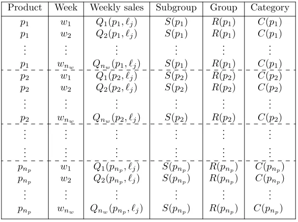
Now the notation is defined, we can give an overview of the available sales data. Table 1 illustrates the sales data of all productsP over the weeks of W:
Product Week Weekly sales Subgroup Group Category
p1 w1 Q1(p1, `j) S(p1) R(p1) C(p1)
p1 w2 Q2(p1, `j) S(p1) R(p1) C(p1)
..
. ... ... ... ... ...
p1 wnw Qnw(p1, `j) S(p1) R(p1) C(p1)
p2 w1 Q1(p2, `j) S(p2) R(p2) C(p2)
p2 w2 Q2(p2, `j) S(p2) R(p2) C(p2)
..
. ... ... ... ... ...
p2 wnw Qnw(p2, `j) S(p2) R(p2) C(p2)
..
. ... ... ... ... ...
..
. ... ... ... ... ...
pnp w1 Q1(pnp, `j) S(pnp) R(pnp) C(pnp)
pnp w2 Q2(pnp, `j) S(pnp) R(pnp) C(pnp)
..
. ... ... ... ... ...
[image:8.612.155.458.107.333.2]pnp wnw Qnw(pnp, `j) S(pnp) R(pnp) C(pnp)
Table 1: Available sales data of all productsP.
As input for the revenue maximizing assignment problem, we need the expected weekly revenues Y(pi, `j), obtained from the expected weekly salesX(pi, `j) of a productpi∈P(Cx) on all locations`j ∈L(Cx).
Sec-tion 4.1 clarifies the method which is used to obtain the expected weekly revenuesY(pi, `j)∀pi∈P(Cx), `j∈ L(Cx).
3.2
The categorized assignment problem with additional feasibility
require-ments
The previous section described the notation which we will use throughout this report and the data which is available to predict the expected weekly revenues.
Section 3.2.1 starts with the explanation how the assignment problem of the entire store is decomposed in the assignment problem per category. After that, Section 3.2.2 will describe the additional feasibility requirements that are applicable to the categorized assignment problem and Section 3.2.3 will provide the final statement of the categorized assignment problem.
3.2.1 Decomposition of the assignment problem of the store into the categorized assignment problem
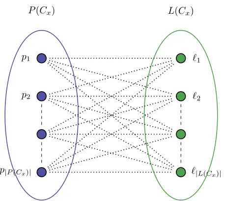
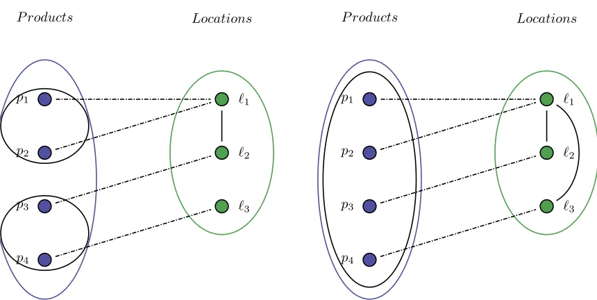
A categorized assignment problem aims to find the revenue maximizing assignment of products P(Cx) to locationsL(Cx) for a categoryCxwhich satisfies some additional feasibility requirements. The representation of productsP(Cx) and locationsL(Cx) can be visualized as a bipartite graphGx= (P(Cx)∪L(Cx), E) as
p1
p2
p|P(Cx)|
`1
`2
`|L(Cx)|
[image:9.612.193.423.80.284.2]P(Cx) L(Cx)
Figure 1: Categorized assignment problem: bipartite graphGx= (P(Cx)∪L(Cx), E),|E|=|P(Cx)|·|L(Cx)|.
The weight of every edge (pi, `j) ∈ E represents the expected weekly revenue of product pi on location
`j. In the categorized assignment problem it has to be determined which edge to choose for each product, i.e. to which location `j ∈ L(Cx) each product pi ∈ P(Cx) will be assigned to. The products and
loca-tions of each category can be visualized in this way. Only the size and weights of the graph differ per category.
p1
p2
p3
p4
p5
pnp
`1
`2
`3
`4
`5
`n`
Products Locations
P(C1)
P(C2)
P(Cnc)
L(C1)
L(C2)
[image:10.612.163.453.72.423.2]L(Cnc)
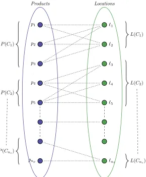
Figure 2: Assignment problem of the entire store: bipartite graph G= (P ∪L, E), with |P| =np,|L| =
n`,|E|= Pnc
x=1|P(Cx)| · |L(Cx)|.
In Figure 2 an example is given of a decomposition of the assignment problem of the store intonc catego-rized assignment problems. The upper three products and upper two locations belong to the first category. In determining the revenue maximizing solution of the store, the solution for each categorized assignment problem can be computed individually.
The next section will describe the additional requirements an assignment has to satisfy for the catego-rized assignment problem of categoryCx. We will explain this for some category Cx∈C, whereCx could
be any of the{C1, . . . , Cnc}categories.
3.2.2 Feasibility constraints
In determining the revenue maximizing assignment, we have to take into account the requirements for an assignment to be feasible. This section will describe each of those requirements and explains why they are necessary. Section 4 will derive the mathematical formulation of these requirements.
First of all, each location `j ∈ L has a certain capacity A(`j) which indicates the maximum number of
different products that can be assigned to this location. This capacityA(`j) is equal to the highest number
of different products of categoryCxthat have been positioned on location`j in a week.
With the above mentioned in consideration, the first feasibility requirement can be formulated as follows:
Definition 1. Within a feasible solution to the categorized assignment problem, the number of different products to a location`j∈L(Cx)may not exceed its capacity A(`j).
The second requirement concerns the hierarchy of products, subgroups and groups within a categoryCx.
For the convenience of the customer, products of of a certain subgroup or group should be assigned to locations ofL(Cx) that are in close proximity to each other. In this way a store layout becomes reasonable and intuitive for the customers of the store.
However, close proximity can be interpreted differently regarding a subgroup or a group. To illustrate this difference, consider the following example:
[image:11.612.187.423.251.412.2]Example 1. Consider the example of a store layout in Figure 3 together with its schematic representation in Figure4.
Figure 3: A physical store layout with six locations illustrated as grey boxes and walkways illustrated as arrows.
`1
`2
`3
`4
`5
`6
Figure 4: Schematic representation of Figure 3.
Within Figure 3, observe that the facing of each location is directed towards the walkways. Location `1 is positioned next to location`2 and they are facing the same walkway. Location`3 is standing with its back to location`1, as well as for location`4 and `2.
Now consider the situation in which the subgroup shavers, from the example of Section3.1, would be assigned to location`1and`3. A customer could experience this assignment as unreasonable because the customer has to walk around the locations to the other walkway to compare products of the subgroup shavers. So products of a certain subgroup should be positioned on the same location or locations that are next to each other and facing in the same direction. On the other hand, it might be more reasonable to assign different subgroups of a certain group to location `1 and`3 because products of different subgroups may be positioned more widely from each other and the locations a group is assigned to, cover a larger area of the store layout than the locations a subgroup is assigned to.
As Example 1 illustrates, there is a difference in close proximity regarding subgroups and groups.
cate-locations are in close proximity to each other regarding subgroups and groups respectively. The edges Ee
illustrate which locations are in close proximity to each other regarding subgroups, i.e. which locations are adjacent regarding subgroups. The same applies for the edges E within Ux regarding groups, i.e. which
locations are adjacent regarding groups.
As suggested in Example 1, an edge e = (`j, `k)∈ Ee only exists if the locations `j and `k are positioned
next to each other within the store layout and if they are facing in the same direction. Regarding groups, an edgee∈E exists if one of the following scenario’s is applicable:
1. two locations are positioned next to each other and they are facing in the same direction.
2. two locations are facing in the opposite direction, with a walkway in between.
3. two locations are facing in a perpendicular direction, with a walkway in between.
4. two locations are positioned back to back.
Thus, an edge e ∈ Ee only exists if the first scenario is applicable and an edge e ∈ E if one of the four
scenario’s is applicable. For this reasonEe is always a subset ofE: that is, Ee⊆E.
Observe that the graphBx only consists of paths since locations inBx are adjacent if the first scenario is
applicable.
To illustrate how a graphBx andUx is created, observe Figure 5 and Figure 6. They illustrate the graphs Bx andUx respectively, generated by the store layout of Figure 3.
1
2 3
4 5
6
Figure 5: The graphBx= (L(Cx),Ee) which is induced by the layout of Figure 3.
1
2 3
4 5
6
Figure 6: The graphUx= (L(Cx), E) which is induced by the layout of Figure 3.
Observe that withinUx, the locations`1and`2,`3and`4, and`5and`6are adjacent by scenario 1. Location
`3 and`5, and `4 and`6 are adjacent by scenario 2. At last, location`1 and`3, and `2 and`4 are adjacent
by scenario 4. To illustrate when scenario 3 would be applicable, consider you are facing a location`j and you have to rotate 45 degrees and face location`k with a walkway in between.
In order to check whether the assigned locations of a subgroup are positioned in close proximity to each other, the assigned locations of each subgroup must induce a connected subgraph inBx, for each subgroup.
Similarly, the assigned locations of each group must induce a connected subgraph inUx, for each group.
Definition 2. Within a feasible solution to the categorized assignment problem, the allocated locations of every subgroup should induce a connected subgraph in graphBx, for each subgraph, and the allocated locations of every group should induce a connected subgraph in graph Ux, for each group.
To give insight how the graphsBxandUx play a role in the feasibility of the solution, consider Example 2.
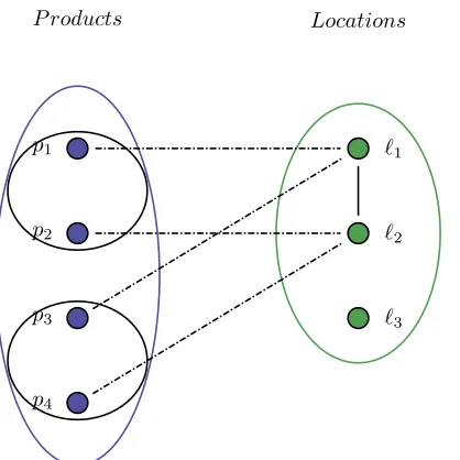
Example 2. Consider the case of assigning the four products of Table2to the locations{`1, `2, `3}of Figure
Product Subgroup Group
p1 S1 R1
p2 S1 R1
p3 S2 R1
[image:13.612.234.378.71.137.2]p4 S2 R1
Table 2: Example of the properties of the productsP(Cx).
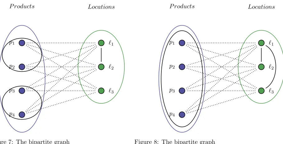
The edges between the locations{`1, `2, `3}of graphBxin Figure5and of graphUxin Figure6can be inserted into the bipartite graph of products and locations as in Figure 7 and Figure 8 respectively. Furthermore products of the same subgroup are circled together in Figure 7 and products of the same group are circled together in Figure8.
p1
p2
p3
p4
`1
`2
`3
[image:13.612.90.545.247.479.2]P roducts Locations
Figure 7: The bipartite graph
Gx= (P(Cx)∪L(Cx), E) with graphBx inserted.
p1
p2
p3
p4
`1
`2
`3
P roducts Locations
Figure 8: The bipartite graph
Gx= (P(Cx)∪L(Cx), E) with graphUx inserted.
As stated in Definition2, the locations allocated to each subgroup should form a connected subgraph in graph
Bx. The same applies for the locations allocated to each group regarding graph Ux. To illustrate that a feasible solution should satisfy these requirements, consider a feasible assignment that is depicted in Figure
p1
p2
p3
p4
`1
`2
`3
[image:14.612.183.512.86.313.2] [image:14.612.90.299.89.298.2]P roducts Locations
Figure 9: Feasible solution regarding subgroups since the locations allocated to subgroupS1 form a
connected subgraph inBx by the edge between`1
and`2. The same applies for the locations allocated
to subgroupS2.
p1
p2
p3
p4
`1
`2
`3
P roducts Locations
Figure 10: Feasible solution regarding groups since the locations allocated to the one existing groupR1
form a connected subgraph inUx by the edge between`1 and`2.
We illustrate the assignment in two figures because the assignment illustrated in both figures should be feasible regarding subgroups and groups. As explained in the figures, this assignment is feasible because the locations allocated to each subgroup form a connected subgraph in graph Bx and the locations allocated to each group form a connected subgraph in graph Ux.
p1
p2
p3
p4
`1
`2
`3
[image:15.612.93.523.85.301.2]P roducts Locations
Figure 11: Infeasible solution regarding subgroups since the locations allocated to subgroupS2 do not
form a connected subgraph in graphBx.
p1
p2
p3
p4
`1
`2
`3
P roducts Locations
Figure 12: Feasible solution regarding groups since the locations allocated to groupR1 form a connected
subgraph inUx.
As explained in Figure 11, the assignment illustrated in Figure 11 and Figure 12 is infeasible because the locations allocated to subgroup S2 do not form a connected subgroup inBx since location `2 and `3 are not connected inBx.
Now all the feasibility requirements are formulated, the next section will describe the definition of the categorized assignment problem with the additional feasibility requirements.
3.2.3 Definition of the categorized assignment problem with feasibility requirements
Recall that the goal is to find a feasible revenue maximizing assignment of products P(Cx) to locations
L(Cx) for every categoryCx∈C. These revenue maximizing assignments for the categories{C1, . . . , Cnc}
together will form the revenue maximizing assignment of the store. An illustrated example of this is given in Figure 2. In the previous section we described the requirements for a feasible solution to the categorized assignment problem. Therefore we now can formally define the categorized assignment problem, which we will refer to as theCA-problem:
Definition 3. The categorized assignment problem
Given a set of products P(Cx) with corresponding subgroups S(Cx) and groups R(Cx), a set of locations
4
Estimating the expected weekly revenues and an Integer Linear
Program formulation to solve the
CA
-problem.
This section explains how to compute the revenue maximizing assignment for the categorized assignment problem formulated in Definition 3. Section 4.1 describes the way the expected weekly revenues are predicted, which are needed as input for the categorized assignment problem. Section 4.2 outlines the algorithm which is used to find the revenue maximizing assignment to theCA-problem.
4.1
Estimate the expected weekly revenue for the categorized assignment
prob-lem
This section explains how the expected weekly salesX(pi, `j)∀pi∈P(Cx), `j ∈L(Cx) are predicted. These
are necessary to predict the expected weekly revenuesY(pi, `j), which are simply predicted by multiplying
the expected weekly salesX(pi, `j) by its gross profitg(pi).
To predict the expected weekly sales, we use the historical sales of products on their historical locations as depicted in Table 1. However, the historical locations of almost every product is a subset of the locations it can be assigned to, L(Cx). Estimating the expected weekly sales of a product on a historical location sounds reasonable, but estimating the expected weekly sales of a product on a location it never stood before, requires another approach.
Before we will explain how we predict the expected weekly sales X(pi, `j) ∀pi ∈ P(Cx), `j ∈ L(Cx), we want to address that we are aware of the fact that the expected weekly sales will be estimated by simple methods and that these methods are imperfect. This is caused by the quality and characteristics of the available historical weekly sales data, depicted in Table 1. That is, it is difficult to fit a distribution to the historical weekly sales of a product because many products have not been sold for weeks and when they were sold, the quantity varied a lot. Furthermore, given the available sales data, the only features we were able to use, are the location and the product itself. The quality and characteristics of the data will be further discussed in Section 7.
Now we shall explain the different approaches to predict X(pi, `j), depending on whether `j is a histori-cal or non-historihistori-cal location of productpi.
Section 4.1.1 will provide a method to predictX(pi, `j) on historical locations of each productpiand Section 4.1.2 will explain the method wherebyX(pi, `j) is predicted on non-historical locations of productpi.
4.1.1 Estimate the expected weekly sales of products on historical locations
We are interested in estimating the expected weekly sales X(pi, `j) for all productspi ∈P(Cx) on its
his-torical locations `j ∈ Li(Cx) using the historical weekly sales data. This section will propose two simple
methods that will predict these expected weekly sales of products on its historical locations. The first method is taking the average of all historical weekly sales of a product pi on its historical location`j. The second
method is to use a Poisson regression with the productpi and historical location`j as predictors.
After the explanation of both methods, we will validate and argue which method is the most appropriate to use and conclude with the formula we will use to predict the expected weekly sales of products on its historical locations.
In the following two paragraphs the proposed methods will be explained.
Taking the average
Taking the average of the historical weekly sales of a product in order to predict the expected weekly sales is intuitive and applicable. Consider the following example to illustrate this:
Product Week Weekly sales Location Subgroup Group Category
p2 w1 3 `3 S1 R3 C1
p2 w2 0 `3 S1 R3 C1
p2 w3 1 `3 S1 R3 C1
p2 w4 0 `5 S1 R3 C1
p2 w5 3 `5 S1 R3 C1
[image:17.612.131.483.73.163.2]p2 w6 4 `5 S1 R3 C1
Table 3: Historical sales of a certain product.
The prediction of the expected weekly salesX(p2, `3)andX(p2, `5)is executed as follows:
ˆ
X(p2, `3) =
1 3
3
X
t=1
Qt(p2, `3) = 1
1 3
ˆ
X(p2, `5) =
1 3
6
X
t=4
Qt(p2, `5) = 2
1 3.
So given these historical sales, it is expected that the weekly sales of product p2 on location `3 and `5 will amount to 113 and 213 respectively.
Recall that the weeks a productpi was positioned on its historical location`j, is denoted byW(pi, `j).
In general, using the average of historical sales to estimate the expected weekly sales of a productpi∈P(Cx)
on a historical location`j ∈Li(Cx), is done in the following way:
ˆ
X(pi, `j) = P
wt∈W(pi,`j)Qt(pi, `j)
|W(pi, `j)| . (1)
Poisson regression
The second method which can be used to predict the expected weekly sales of a product on its historical location is a Poisson regression. A regression is utilized to reflect the relationship between a response variable and a set of predictors. In our case the response variable is the weekly sales of a product on its historical location and the predictors are the locations and the products. To use a Poisson regression to predict the expected weekly salesX(pi, `j), we have to assume that the weekly sales of a product on its historical location
follow a poisson distribution [8].
Since the weekly sales of a product on its historical location can be described as a count of events in the time interval of a week, the weekly sales might follow a Poisson distribution [9]. Therefore it is a reasonable attempt to predict the expected weekly sales by a poisson regression.
However, it appears that the available historical weekly sales of a product does not fit the Poisson distri-bution very well due to the poor quality of the data. Nevertheless, we want to compare the approach of taking the average with another method and therefore we do perform a poisson regression and analyze the performances of both methods.
Where an ordinary least squares (OLS) regression aims to model the expected value of the response variable on itself, a Poisson regression aims to model the natural log of the expected value of the response variable. To understand what a Poisson regression precisely does to predict the expected weekly sales, we will give two examples. In Example 4 only the location is used as a predictor and in Example 5 both the location and the product are a predictor.
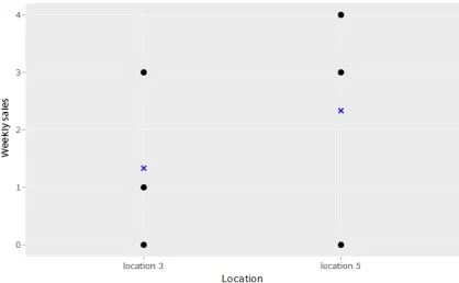
Figure 13: Visualization of weekly sales of a product on two locations illustrated as dots, together with the expected weekly sales per location illustrated as crosses.
We predict the expected weekly salesX(p2, `j)with the location`j ∈L2(Cx)as predictor. The product pi is
not a predictor yet, because in this example we only possess over the sales data of productp2.
Since the Poisson regression models the natural log of the expected weekly sales, the model will be of the form:
ln( ˆX(p2, `j)) =β0+βj+µ2,j ⇐⇒ Xˆ(p2, `j) = eβ0+βj+µ2,j.
The Poisson regression reveals the relationship between the expected weekly sales and the locations of this productp2. To notice the effect a location has on the expected weekly sales, some location has to be selected as a benchmark such that the other locations can be compared to this benchmark location. In our example location `3 is the benchmark location, so the expected weekly sales of product p2 on location `3 is given by
ˆ
X(p2, `3) = eβ0. The effect in weekly sales of changing location from`3 to`5 is given by eβ5+µ2,5 and hence
ˆ
X(p2, `5) = eβ0+β5+µ2,5. These expected weekly sales are denoted as crosses in Figure13. We will explain how the coefficients such as β0,β5 andµ2,5 are estimated if we add the product as a predictor.
So with one product, the Poisson regression with the location as predictor is given by:
ˆ
X(pi, `j) = eβ0+βj+µi,j.
For every location`j that is not equal to the benchmark location, there is a coefficientβj andµi,jthat will correct for a change in location from the benchmark location to`j.
Hereby the Poisson regression with the product and location as categorical predictor will be of the form:
ln( ˆX(pi, `j)) =γ0+αi+βj+µi,j ⇐⇒ Xˆ(pi, `j) =eγ0+αi+βj+µi,j.
(2)
For the benchmark productpiand benchmark location`j, the expected weekly sales are given by ˆX(pi, `j) = eγ0. With Equation 2 a change in product and change in location are considered dependent from each other.
This also is the case since the sale of a productpi occurred when it was positioned on its historical location
`j. Therefore we make a correction for a change in productpi with coefficient αi, for a change in location
`j with coefficientβj and the interaction of those changed product and location is given by coefficientµi,j. For each product pi ∈P(Cx) and location `j ∈Li(Cx), the coefficients αi, βj and µi,j are determined by the method of maximum log-likelihood [8].
Within the program R, we predicted the expected weekly revenuesX(pi, `j) via Equation 1 and Equation
2. It turns out that both approaches resulted in the exact same predictions. It appears that by includ-ing the interaction coefficientµi,j in Equation 2, the Poisson regression predicts the same expected weekly
sales as the expected weekly sales predicted by taking the average. A proof of this is included in AppendixA.
Since we want to compare the approach of taking the average with another approach, we will perform a Poisson regression with the product and location as predictor under the assumption that the product and location are independent from each other. So the interaction coefficient is not included. Then the Poisson regression to predict the expected weekly sales is given by:
ln( ˆX(pi, `j)) =γ0+αi+βj
⇐⇒ Xˆ(pi, `j) =eγ0+αi+βj. (3)
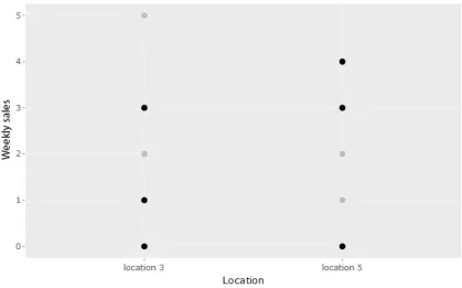
To demonstrate how the Poisson regression of Equation 3 works, consider Example 5:
[image:19.612.94.513.439.700.2]In this example product p2 and location `3 are chosen as the benchmark product and location. Hence,
ˆ
X(p2, `3) = eγ0 is the expected weekly sales of product p2 on its historical location `3. The expected weekly sales X(p2, `5), X(p4, `3) and X(p4, `5) are given by Xˆ(p2, `5) = eγ0+β5, Xˆ(p4, `3) = eγ0+α4 and
ˆ
X(p4, `5) = eγ0+α4+β5.
So using the Poisson regression, Equation 3 is used to predict the expected weekly sales of products on its historical locations.
Observe that a correction βj that is made for a change in location `j from the benchmark location, is based on the sales of the products that were positioned on this location`j in the past. So the correctionβj
is actually induced by the products that were sold on location`j, and not only by the characteristics of the location itself. This will be further discussed in Section 7.
Computational validation
We proposed two methods to predict the expected weekly sales of products on historical locations. In order to determine which method we shall use, a validation on the predictions via Equation 1 and Equation 3 will be executed. The program R is used for this.
We are aware of the fact that given the quality of the data, we can not be very certain about the con-clusions we can draw from the validations. However, it does give an indication about the performance of both methods.
For the validation we split the data set D, illustrated in Table 1, into two mutually exclusive subsets, named the training setDtraining and the test set Dtest. We will validate the methods for all productsP to obtain a validation that is applicable for the whole store.
The training set is used to train the model, i.e. to predict the expected weekly salesX(pi, `j)∀pi ∈P, `j∈ Li(Cx). These expected weekly sales can be compared to the actual weekly sales the corresponding product and location included in the test set. In order to validate each expected weekly salesX(pi, `j), every (pi, `j) combination needs to be present in the test set as well as in the training set. Therefore we include 20 % of the weekly sales of each product on its historical location (pi, `j) in the test set, rounded up to an integer. The other 80 % is included in the training set. The training set is therefore defined byDtraining=D\Dtest.
The weeks of historical sales of productpi on historical location`j that are included inDtest are denoted by W(test)(p
i, `j), whereW(test)(pi, `j)⊆W(pi, `j).
In the validation, each prediction X(pi, `j) will be compared to every occurringQt(pi, `j) inDtest. During
the validation a metric has to be chosen to compare the predictions with the real weekly sales. For this validation we will use the mean absolute error (MAE) to determine the performance of both methods. The performance of a model will then be given by:
M AE=
P pi∈P
P
`j∈Li(Cx)
P
wt∈W(test)(pi,`j)
ˆ
X(pi, `j)−Qt(pi, `j)
P
pi∈P
P
`j∈Li(Cx)|W
(test)(pi, `j)| . (4)
Recall thatQt(pi, `j) is the number of sales of productpi on its historical location`j in weekwt.
Thus, the MAE is the average deviation between the predicted expected weekly sales and the historical weekly sales over all observations of products on its historical locations that are included inDtest.
IfX(pi, `j) is predicted by the Poisson regression, we denote the MAE byM AEP oissonand if the average is used to predictX(pi, `j), the MAE is denoted byM AEaverage.
To compare the performance of the methods as objective as possible, we need to validate the predictions of the methods on different test sets, i.e. validate whether the predictions of the methods fit different samples of reality.
Therefore we will compute twenty different samples of D from whichDtest and thereby alsoDtrain is
are depicted in Table 4 together with the mean of the historical sales of the test setDtest of each run.
run M AEP oisson M AEaverage Mean of historical sales
1 1.1576 1.1762 1.0302
2 1.0995 1.1102 1.0532
3 1.2157 1.2329 1.1671
4 1.0877 1.0859 1.0818
5 1.1413 1.1495 1.0741
6 1.0602 1.0786 1.1732
7 1.1471 1.1777 1.1980
8 1.1317 1.1389 1.0238
9 1.1586 1.1841 1.2608
10 1.1088 1.1198 1.1745
11 1.1140 1.1232 1.1149
12 1.1098 1.1142 1.1628
13 1.1028 1.1314 1.1538
14 1.0771 1.0901 1.1276
15 1.1470 1.1688 1.2687
16 1.1239 1.1411 1.1112
17 1.1391 1.1570 1.1239
18 1.0961 1.0948 1.1366
19 1.0332 1.0575 1.0887
[image:21.612.162.451.107.361.2]20 1.1238 1.1395 1.1642
Table 4: M AEP oisson andM AEaveragefor 20 runs.
In order to interpret each MAE, the last column is added which indicates the mean of the historical sales of the corresponding Dtest. In each run, the MAE represents the mean error the predictions deviate from
the mean sales. It can be noticed that in most of the runs the deviation is almost equal to the mean. This confirms the remark at the beginning of this section that the methods will be imperfect due to the quality of the data that is available.
Moreover, it can be observed that the differences between M AEP oisson and M AEaverage are negligible. We already argued that the available sales of the historical weekly sales of a product on its historical lo-cation can not be fitted by a Poisson distribution very well. Due to this and the fact that the difference in performance between the Poisson regression and taking the average is negligible, we do not predict the weekly sales on historical locations by a Poisson regression as in Equation 3.
For taking the average, the only requirement is that the average of weekly sales of a product exist. This is the case since the weekly sales are non-negative and bounded.
Therefore we will use the average to predict the expected weekly sales of products on its historical locations.
In the next section we will provide the method by which the expected weekly sales of products on its non-historical locations are estimated. In this method we pretend like the products of a group are identical and therefore use the historical weekly sales of the group R(pi) to predict the expected weekly sales of a product pi on the non-historical locations of the group R(pi). Section 4.1.2 explains this in detail, but to compare the expected weekly sales of a product objectively over all locations L(Cx), we will also use the historical weekly sales of a groupR(pi) to predict the expected weekly sales of the historical locations of the groupR(pi).
Thus, instead of Equation 1, we will use the average of the weekly sales of groupR(pi) to predictX(pi, `j) for locations`j∈S
pf∈R(pi)Lf(Cx):
P p ∈R(p)
P
4.1.2 Estimate expected weekly sales of products on non-historical locations
So far, we only discussed how to predict the expected weekly sales of products on their historical locations. As mentioned at the beginning of Section 4.1, we are aware of the fact that the methods we use to predict the expected weekly sales are imperfect. This applies to the predictions on historical locations of products, but certainly also to the predictions on non-historical locations of products.
Section 3.2.2 describes how the graphs Bx and Ux are formed for each category, which are representa-tions of the connectivity between the locarepresenta-tions L(Cx) regarding subgroups and groups respectively. If we would like to predict the expected weekly sales of a productpi on a location `k it never stood before, the product might have been positioned on locations that are in close proximity, i.e. locations that are adjacent to`k in Ux. However, most products have stood on one or two locations in available dataset. As mentioned at the end of Section 4.1.1, it is more interesting to look at the products of its group R(pi), i.e. products
that are similar topi, since it is reasonable that these products together have stood on more locations than
the productpi itself.
Therefore the expected weekly sales of productpion the historical locations of its groupR(pi), are predicted
by the average sales of its group on this location. We do not take the average of the weekly sales of the prod-uct itself anymore because we want to compare the expected weekly revenues of a prodprod-uct, predicted from the expected weekly sales, objectively over all locations. This can only be done if we use the historical sales of a group for all locations. Otherwise, the best performing products of a group will be assigned to one of its historical locations and the worst performing products of a group will be assigned to non-historical locations.
To predict the expected weekly sales on non-historical locations, we will use a weighted average, based on the idea of the kriging method, which uses statistical interpolation on spatial data [10]. To predict the sales of a non-historical location of group R(pi), we will use the expected weekly sales of group R(pi) on locations that are in close proximity to the non-historical location of groupR(pi).
Notice that hereafter we will define some new notation in order to explain how this results in a weighted average.
We want to estimateX(pi, `k) for non-historical location`k of product groupR(pi) by using the predictions
ˆ
X(pf, `j) of productspf ∈R(pi) on adjacent locations`j ∈ {L(Cx)|(`k, `j)∈E(Ux)}.
This is done in the following way:
ˆ
X(pi, `k) =
P
`j∈L(Cx)d
(i)
k,jXˆ(pi, `j), ifP`j∈L(Cx)d
(i)
k,j >0 P
`j∈L(Cx) P
pf∈R(pi) P
t∈W(pi,`j)Qt(pf,`j)
P
`j∈L(Cx) P
pf∈R(pi)|W(pf,`j)| , if
P
`j∈L(Cx)d
(i)
k,j = 0
(6)
The clarification of the different cases will be explained after the explanation of the weightsd(k,ji).
These weights d(k,ji) denote the normalized closeness between location`j and `k regarding group R(pi) and thereforeP
`j∈L(Cx)d
(i)
k,j = 1.
The weightsd(k,ji) are obtained by:
d(k,ji) =
d(k,ji) P
`q∈L(Cx)d (i)
k,q
, ifP
`q∈L(Cx)d
(i)
k,q>0
0, ifP
`q∈L(Cx)d
(i)
k,q= 0
The weight d(k,ji) indicate the closeness between the locations `k and `j regarding group R(pi), by a value
between zero and one. The weights are determined according to the scenario’s that induce the edges inUx,
described in Section 3.2.2. A weight of zero indicates that the location`j is not comparable to`k regarding
regarding groupR(pi):
d(k,ji) =
1, If`j =`k and group R(pi) was positioned on location `j
0.8, If location`j is adjacent to location`k according to scenario 1,
and group R(pi) was positioned on location`j
0.6, If location`j is adjacent to location`k according to scenario 2,
and group R(pi) was positioned on location`j
0.4, If location`j is adjacent to location`k according to scenario 3,
and group R(pi) was positioned on location`j
0.2, If location`j is adjacent to location`k according to scenario 4,
and group R(pi) was positioned on location`j
0, If there is none of the four scenario’s applicable to locations`j and`k,
or groupR(pi) was not positioned on location`j.
Note thatd(k,ji) = 1 is only added for completeness because this weight will never be used. If groupR(pi) was
positioned on location`j=`k, thenX(pi, `k) is predicted by Equation 5.
The weightsd(k,ji) are based on the expertise of a data expert in the field of retail because we could not compute reliable correlations between locations due to the quality of the data. This will also be discussed in Section 7.
Further observe that the weights d(k,ji) depend on the group R(pi) because not every group is positioned on every location ofL(Cx). To illustrate this, consider the case that location`j might be adjacent to`k in graph Ux, but if the group of the productpi which we try to predict, was never positioned on location`j,
this location can not be used for the expected weekly sales of productpi on non-historical location`k. For
a product of a different group, this group might be positioned on location`j and this location can be used
to estimate the expected weekly sales. Therefore a weightd(k,ji) depends on the groupR(pi).
At last, consider the case in Equation 6 where the group R(pi) was not positioned on any of the adja-cent locations of `k in the past. Then there is no location to use for the estimation of the expected weekly
sales X(pi, `k) and therefore P`j∈L(Cx)d
(i)
k,j = 0 and thus P
`j∈L(Cx)d
(i)
k,j = 0. In this case, the expected
weekly salesX(pi, `k) will be predicted by the average sales of the groupR(pi) over all locations ofL(Cx).
So far we have a method to predict the expected weekly sales X(pi, `j) for the historical locations and
non-historical locations of its groupR(pi). As input for computing the revenue maximizing assignment of
categoryCx, we need the expected weekly revenuesY(pi, `j) for all productsP(Cx) on locationsL(Cx). The
expected weekly revenuesY(pi, `j) are predicted by multiplying each expected weekly salesX(pi, `j) by its
gross profitg(pi):
ˆ
Y(pi, `j) =g(pi)·Xˆ(pi, `j) ∀pi∈P(Cx), `j∈L(Cx). (7)
Summarizing, the expected weekly sales of a product pi on the historical locations of its groupR(pi) are predicted by the average sales of the groupR(pi) on this location:
ˆ
X(pi, `j) = P
pf∈R(pi)
P
wt∈W(pi,`j)Qt(pf, `j)
P
pf∈R(pi)|W(pf, `j)|
∀`j ∈ [
pf∈R(pi)
Lf(Cx).
locations that are adjacent to a non-historical location of groupR(pi), the expected weekly sales of product
pion this location will be the average sales of the groupR(pi) over all locationsL(Cx):
ˆ
X(pi, `k) =
P
`j∈L(Cx)d
(i)
k,jXˆ(pi, `j), if P
`j∈L(Cx)d
(i)
k,j >0 P
`j∈L(Cx) P
pf∈R(pi) P
t∈W(pi,`j)Qt(pf,`j)
P
`j∈L(Cx) P
pf∈R(pi)|W(pf,`j)| , if
P
`j∈L(Cx)d
(i)
k,j = 0
With the expected weekly salesX(pi, `j) and gross profitsg(pi), we can predict the expected weekly revenues
Y(pi, `j):
ˆ
4.2
Compute the revenue maximizing assignment to the categorized assignment
problem
This section will explain how to obtain the revenue maximizing assignment for the CA-problem, defined in Definition 3. It appears that theCA-problem is NP-hard, which will be proved in Section 4.2.1. After that, Section 4.2.2 will provide the Integer Linear Program whereby the revenue maximizing assignment for the
CA-problem is computed.
4.2.1 NP-hardness
To show that the CA-problem is NP-hard, we will prove that a simplified version of the CA-problem is NP-hard. If this holds, then theCA-problem itself is also NP-hard.
We will derive to this simplified version in two steps. First assume that the requirement of Definition 2 is only considered for groups, that is that the locations allocated to every group should form a connected subgraph in Ux. So focused on one group, the aim is to assign products of this group to locations such that these locations form a connected subgraph in the corresponding graph Ux and the number of assigned products to a vertex does not exceed its capacity. This can be defined mathematically as the following problem:
Capacitated connected subgraph problem (CCS)
Given a graph Ux = (V, E) with vertex capacities A(v), vertex weightsw(v) and a positive integer k, find a connected subgraph (V0, E0) with vertex loads r(v) such that P
v∈V0r(v) =k, r(v)≤A(v)∀v∈V0 and
P
v∈V0r(v)·w(v) is maximized.
One may think of k as the number of products of some group that have to be assigned. The vertices
V ofUxcorrespond to the locationsL(Cx). The vertex loadr(v) is the number of products which is assigned
to vertexvand trivially, this number of products may not exceed its capacityA(v). The vertex weightsw(v) correspond to expected weekly revenue of products to locations. Here the expected weekly revenue of every product on a locationv has the same weightw(v), so this also is a simplification of theCA-problem. Now we will simplify the CCS-problem by setting all vertex capacities equal to one. Actually we neglect the capacity constraint by allowing a vertex to be allocated to only one product and therefore the vertex loadsr(v) become unnecessary. With this simplification we will study a well known problem in the literature:
Maximum weight connected subgraph (MWCS)
Given a graph G = (V, E) with vertex weights w(v) and a positive integer k, find a connected subgraph
H = (V0, E0) with|V0| ≤ksuch thatP
v∈V0w(v) is maximized.
Below we will provide a proof to show thatM W CS is a NP-hard problem even ifw(v)∈ {0,1} ∀v∈V [11]. We do this by using a special case of the well known Steiner tree problem, which is a NP-hard problem [12]:
Steiner Tree (ST)
Given a graphG= (V , E),R⊆V, find a treeT = (V0, E0) inGthat spans R with a minimum number of
vertices|V0|.
We will prove that M W CS with binary vertex weights is NP-hard by showing that the decision version ofM W CS is NP-complete.
Theorem 1. The decision version of the M W CS problem is NP-complete, even if the vertex weights are restricted to be binary: w(v)∈ {0,1} ∀v∈V.
Proof.
The decision version of theM W CS with binary vertex weights is formulated as follows:
First, it is not hard to see that the decision version of theM W CSis in NP. Given a subgraphH = (V0, E0) of an instance ofM W CS, it can be decided in polynomial time whether this subgraphH satisfies the con-ditions|V0| ≤k,w(H)≥z and whether the subgraphH is connected [13].
The decision version of theST problem is as follows:
Given a graphG= (V , E), R⊆V, an integerl ≥ |R|, is there a treeT = (V0, E0) inGthat spans R with
|V0| ≤l ?
To reduce this problem to the decision version of the M W CS problem, we introduce the polynomial-time computable mapping f :IST →IM W CS that maps every instance of the Steiner tree to an instance of the
M W CS. If we can prove that this mapping maps every yes-instance ofIST to a yes-instance ofIM W CS and idem dito for every no-instance, then we have found a reduction fromST toM W CS.
LetG= (V , E),R⊆V, an integerl≥ |R|be an instance ofIST. The mappingf is then defined as follows:
1. Create a node-weighted graphG= (V, E), withV =V,E =E and vertex weights:
w(v) =
(
1, ∀v∈R
0, ∀v∈V \R
2. z=|R|,k=l.
Consider a yes-instance ofIST: A Steiner treeT ofqvertices (q≤l) andq−1 edges (sinceT is a tree) that spans all vertices ofR. Now consider this treeT as the subgraphH, that isH =T.
Then in G = (V, E) this tree H contains less than or equal to k vertices and w(H) ≥z since all vertices withw(v) = 1 are contained in T by construction. Since a tree is a connected subgraph,H is a connected subgraph. So every yes-instance ofIST will be mapped to a yes-instance ofIM W CS.
Consider a no-instance of IST: There is no tree T = (V0, E0) in G with |V0| ≤ l = k that spans all R
vertices. This means that all Steiner trees inGcontain|V0|> kvertices. So inG, any connected subgraph
H with a weightw(H)≥zcontains more thankvertices.
We show this by contradiction. Assume that there is a connected subgraph H = (V0, E0) in G with
|V0| ≤ k = l and w(H) ≥ z = |R| , then in G there should be a tree T = (V0, E0) that spans R with
|V0| ≤l because of the following:
1. If the connected subgraph H described above already is a tree, T =H would have been a tree in G
that spans Rand contains|T(V0)| ≤lvertices.
2. If the connected subgraphH described above is not a tree and thus contains one or more cycles, then we can remove edges fromH under the condition thatH remains connected until eventually a treeT
is obtained. By this,T would be a tree inGthat still spans Rand still contains|T0(V0)| ≤l vertices.
In both cases, this leads to a contradiction since we assumed such a Steiner tree did not exist inG. So every no-instance ofIST will indeed be mapped to a no-instance of IM W CS.
Thus, we can map every yes-instance of IST to a yes-instance of IM W CS and map every no-instance of IST to a no-instance ofIM W CS in polynomial time.
Since ST is a NP-hard problem and we found a polynomial-time computable reduction from the decision version ofST to the decision version ofM W CS, which is in NP, we can conclude that the decision version
ofM W CS is NP-complete.
solve theCA-problem. The following section describes the way this ILP is created and ends with the ILP as a whole.
4.2.2 Integer Linear Program to solve theCA-problem
We are going to set up an ILP to solve theCA-problem.
First of all, we will denote the expected weekly revenuesY(pi, `j) byw(pi, `j)∀pi∈P(Cx), `j ∈L(Cx). Furthermore, we have to indicate whether a product is assigned to a location within a solution. Therefore we define the following binary variable:
x(pi, `j) =
(
1, When productpi is assigned to location`j
0, Otherwise.
In the assignment every product should be assigned to exactly one location. Using the variablex(pi, `j), this requirement can be formulated as the following constraint:
Allocation constraint.
X
`j∈L(Cx)
x(pi, `j) = 1∀pi∈P(Cx). (8)
Furthermore Section 3.2.2 already describes the feasibility constraints that a solution has to satisfy. As said in Definition 1, the number of assigned products to a location`j, may not exceed its capacityA(`j). This is translated into the following constraint:
Capacity constraint.
X
pi∈P(Cx)
x(pi, `j)≤A(`j)∀`j∈L(Cx). (9)
Recall that every productpi belongs to a subgroupS(pi) and a groupR(pi). Thus, besides a set of products
P(Cx), every categoryCx also contains a set of subgroups and groups denoted byS(Cx) andR(Cx) respec-tively.
In addition to the capacity constraint, it has to be ensured that the products of a subgroup are assigned to locations that form a connected subgraph inBx. Before stating this in a constraint, we first need a variable that indicates whether a subgroupSh∈S(Cx) is assigned to a location`j:
y(Sh, `j) = (
1, When subgroup Shis assigned to location `j
0, Otherwise.
Whether a subgroup is assigned to a location`j, only depends on the fact whether a product of this subgroup is assigned to location`j. If one or more products of the subgroup are assigned to location`j, the subgroup is also assigned to location`j. If none of the products of the subgroup is assigned to location`j, the subgroup itself is neither assigned to location`j. To force this, we use the following two constraints:
Coupling constraints.
y(Sh, `j)≥x(pi, `j)∀Sh∈S(Cx), pi∈Sh, `j ∈L(Cx) (10)
y(Sh, `j)≤ X
pi∈Sh
x(pi, `j)∀Sh∈S(Cx), `j∈L(Cx). (11)
If there is some product pi ∈Sh for which x(pi, `j) = 1, then y(Sh, `j) is free to choose regarding the con-straint of Equation 11 because the value of the sum is one or higher. However, the concon-straint of Equation 10 enforcesy(Sh, `j) = 1 because there is at least one product of subgroupSh that is assigned to location`j.
Thus, the constraints of Equation 10 and 11 forcey(Sh, `j) to be the correct binary value.
Now we know whether a subgroup is positioned on a location or not, it is possible to check if the loca-tions a subgroup is assigned to, indeed form a connected subgraph inBx. As explained in Section 3.2.2, the
graph Bx only consists of paths. Therefore there exists one or no path between two vertices `j and `k in
Bx. The locations located on such a path are defined by the setP(`j, `k). Using each setP(`j, `k), we can formulate the following constraint which checks for every subgroupShif the vertices for whichy(Sh, `j) = 1 form a connected subgraph inBx:
Connectivity constraint regarding subgroups.
y(Sh, `j) +y(Sh, `k)− X lr∈P(`j,`k)
y(Sh, lr)≤1 ∀Sh∈S(Cx),∀`j, `k ∈ {L(Cx)|(`j, `k)∈/E(Bx)}. (12)
Observe that only for the case wherey(Sh, `j) = 1 andy(Sh, `k) = 1 it has to be determined whether the constraint is satisfied. For all other cases the constraint is automatically satisfied since the left-hand side is one or less.
So the constraint verifies for each pair of vertices {(`j, `k)|(`j, `k) ∈/ E(Bx)} for which y(Sh, `j) = 1 and
y(Sh, `k) = 1, if there is at least one vertex `r ∈ P(`j, `k) for which y(Sh, lr) = 1. If this holds, then the locations a subgroup is assigned to, form a path and thus a connected subgraph in Bx. Note that even if
y(Sh, `j) = 1 andy(Sh, `k) = 1, the constraint does not need to be checked if`j and`k are adjacent vertices inBxbecause adjacent vertices are always connected.
To illustrate that the constraint of Equation 12 correctly verifies connectivity of the induced subgraph, consider an extension of the graphBxwhich is depicted in Figure 5 of Section 3.2.2:
1
2 3
4 5
6
7
Figure 15: An extended version of the graphBx= (V,Ee) of Figure 5.
We added a seventh vertex to create the pair (`5, `7) where the vertices are reachable but not adjacent.
Consider the case that y(Sh, l5) = 1 and y(Sh, l7) = 1, but y(Sh, l6) = 0 for some Sh ∈ S(Cx). With
P(l5, l7) = {l6}, the constraint of Equation 12 will not be satisfied since y(Sh, l6) = 0 and therefore the
left-hand side of the constraint is two, which is higher than one.
Ify(Sh, l5) = 1,y(Sh, l7) = 1 andy(Sh, l6) = 1, the constraint of Equation 12 is satisfied and the locations
{l5, l6, l7} the subgroupSh is assigned to, indeed form a connected subgraph inBx.
Secondly, consider the case that y(Sh, l5) = 1, y(Sh, l3) = 1, then constraint 12 will be violated since
P(l3, l5) ={∅}because`3and`5are not reachable. Thus, the constraint of Equation 12 is correctly violated
for locations that are not reachable inBx.
Besides the connectivity check for the locations that are allocated to each subgroup, we have to verify whether the locations assigned to each groupRd form a connected subgraph inUx.
To specify whether a group is assigned to a location, we create the variablez(Rd, `j):
z(Rd, `j) =
(
1, When groupRdis assigned to location `j
0, Otherwise.
to the constraints of Equation 10 and 11:
Coupling constraints.
z(Rd, `j)≥y(Sh, `j)∀Rd∈R(Cx), Sh∈Rd, `j∈L(Cx) (13)
z(Rd, `j)≤ X Sh∈Rd
y(Sh, `j)∀Rd ∈R(Cx), `j∈L(Cx). (14)
Now we know whether a group is assigned to a location inUx, we can focus on the connectivity of all the locations a group Rd is assigned to. In comparison to Bx, inUx there might exist several paths between vertices`jand`kbecauseUxcan contain cycles. Therefore the constraint of Equation 12 should be adjusted in order to check connectivity regarding groups.
To specify the paths corresponding to locations`j and`k, we first create the set that consists of the paths between every two vertices inUx, i.e. the set that contains all paths of Ux: that is, T ={t1, t2, . . . , tnt}.
Here a path tm ∈ T contains the vertices `j ∈ L(Cx) this path tm consists of without the source and destination vertex of the path. These paths can be found using a depth-first search [14]. The paths within
Ux corresponding to source`j and destination`k are denoted by the setT(`j, `k) and is a subset ofT: that
is,T(`j, `k)⊆T.
Comparable to the constraint of Equation 12, for every group Rd we want to check if any two locations
(`j, `k) for whichz(Rd, `j) = 1 andz(Rd, `k) = 1, are connected via vertices that are also assigned to group Rd, i.e. if there is a path tm∈T(`j, `k) where all vertices of this path are also assigned to Rd. To specify whether this holds for a given pathtm∈T and groupRd, we introduce the following variable:
γ(tm, Rd) =
(
1, Ifz(Rd, `j) = 1 for all vertices`j∈tm
0, Otherwise.
To forceγ(tm, Rd) to the correct binary value, we need the following two constraints:
Path constraints.
γ(tm, Rd)≤z(Rd, `j)∀Rd ∈R(Cx), tm∈T, `j ∈tm (15)
γ(tm, Rd)≥
X
`j∈tm
[z(Rd, `j)−1]
+ 1∀Rd∈R(Cx), tm∈T. (16)
Ifz(Rd, `j) = 1 for all vertices`j ∈tm, γ(tm, Rd) is free to choose regarding the constraint of Equation 15. However, the right-hand side of the constraint of Equation 16 is equal to one since the summation equals zero. As a result,γ(tm, Rd) is set to one correctly.
If there is a vertex `j ∈ tm for which z(Rd, `j) = 0, γ(tm, Rd) is free to choose regarding the constraint of
Equation 16 since the right-hand side of this constraint is zero or less. However, the constraint of Equation 15 forcesγ(tm, Rd) to be zero sinceγ(tm, Rd)≤0 for the location`j that was not assigned to groupRd.
Now it is correctly specified whether all vertices of a path are assigned to a group, we can model a constraint that verifies for any pair of locations (`j, `k) for whichz(Rd, `j) = 1 and z(Rd, `k) = 1 whether there is a pathtm∈T(`j, `k) for which γ(tm, Rd) = 1 that assures connectivity between`j and`k. If there is such a path for any two locations that are assigned to groupRd, the locations the groupRd is assigned to, form a connected subgraph inUx. This is done by the following constraint:
Connectivity constraint regading groups.
X
t ∈T(` ,` )
γ(tm, Rd)≥1−
1−z(Rd, `j)−
For the case thatz(Rd, `j) = 1 andz(Rd, `k) = 1, the constraint of Equation 17 is only satisfied if there is at least one pathtm∈T(`j, `k) for which all the vertices on this path are assigned to group Rd and thus`j
and`k are connected via this path.
Ifz(Rd, `j) = 0,z(Rd, `j) = 0 or both are zero, the constraint is automatically satisfied since the right-hand
side is zero or less.
With the constraint of Equation 17, we have modelled all the feasibility constraints a solution for theCA -problem has to satisfy.
Briefly summarizing, for a given category Cx, the CA-problem wants to assign the corresponding prod-uctsP(Cx) to the corresponding locationsL(Cx) with the objective to maximize the total expected weekly revenue of the assignmentP
pi∈P(Cx),`j∈L(Cx)x(pi, `j)w(pi, `j).
The locations L(Cx) located in the store layout induce the connectivity graphs Bx and Ux regarding sub-groups and sub-groups respectively. The locations in the revenue maximizing solution that are assigned to a subgroupShshould form a connected subgraph inBxsuch that the products of subgroupShare positioned in close proximity to each other. Comparable, the locations in the revenue maximizing solution that are assigned to a groupRdshould form a connected subgraph inUxsuch that the products of this groupRdare positioned in close proximity to each other.
Furthermore the number of products assigned to a location may not exceed its capacity and every product is assigned to one location only.
The Integer Linear Program as a whole then looks as follows:
max X
pi∈P(Cx)
X
`j∈L(Cx)
w(pi, `j)x(pi, `j)
subject to
X
`j∈L(Cx)
x(pi, `j) = 1 ∀pi∈P(Cx) (Eq. 8)
X
pi∈P(Cx)
x(pi, `j)≤A(`j) ∀`j∈L(Cx) (Eq. 9)
y(Sh, `j)≥x(pi, `j) ∀Sh∈S(Cx), pi∈Sh, `j∈L(Cx) (Eq. 10)
y(Sh, `j)≤ X pi∈Sh
x(pi, `j) ∀Sh∈S(Cx), `j ∈L(Cx) (Eq. 11)
y(Sh, `j) +y(Sh, `k)− X lr∈P(`j,`k)
y(Sh, lr)≤1 ∀Sh∈S(Cx),
`j, `k ∈L(Cx)|(`j, `k)∈/ E(Bx) (Eq. 12)
z(Rd, `j)≥y(Sh, `j) ∀Rd∈R(Cx), Sh∈Rd, `j ∈L(Cx)(Eq. 13) z(Rd, `j)≤
X
Sh∈Rd
y(Sh, `j) ∀Rd∈R(Cx), `j ∈L(Cx) (Eq. 14)
γ(tm, Rd)≤z(Rd, `j) ∀Rd∈R(Cx), tm∈T, `j∈tm (Eq. 15)
γ(tm, Rd)≥ X `j∈tm
z(Rd, `j)−1
+ 1 ∀Rd∈R(Cx), tm∈T (Eq. 16)
X
tm∈T(`j,`k)
γ(tm, Rd)≥1−
1−z(Rd, `j) −
1−z(Rd, `k)∀Rd∈R(Cx),
`j, `k ∈ {L(Cx)|(`j, `k)∈/E(Ux)} (Eq. 17)