Essays in development economics

(1)

warwick.ac.uk/lib-publications

A Thesis Submitted for the Degree of PhD at the University of Warwick

Permanent WRAP URL:

http://wrap.warwick.ac.uk/92086

Copyright and reuse:

This thesis is made available online and is protected by original copyright. Please scroll down to view the document itself.

Please refer to the repository record for this item for information to help you to cite it. Our policy information is available from the repository home page.

(2)

Essays in Development Economics

by

Kerstin Christina Ammon

Thesis

Thesis submitted to the University of Warwick in partial fulfilment for the degree of

Doctor of Philosophy

in Economics

Department of Economics

(3)

List of Tables

2.1 Summary Statistics . . . 13

2.2 Mill Characteristics that Predict Paddy Share . . . 17

2.3 Loans and Inputs Provided Per Hectare Cultivated with Cane . . . 23

2.4 Baseline Specification Including both Prices and Post-1931 Dummy . . . 24

2.5 Baseline Results Using Rain-Fed Paddy Fields Only . . . . 26

2.6 Effect on Fertiliser Consumption . . . 28

A.1 Timeline . . . 75

A.2 Thailand Prices of Rice on World Market . . . 76

A.3 List of Mills . . . 77

A.4 Loans Issued and Inputs Provided - Logged Total . . . 78

A.5 Loans and Inputs Provided - Pre and Post Comparison . . 79

A.6 Loans Issued and Inputs Provided by Type . . . 79

A.7 Baseline Specification Using Rice Prices . . . 80

A.8 Baseline specification with Prefecture-Year Fixed Effects and Linear Mill Trends . . . 81

A.9 Time-varying Treatment Effects . . . 82

A.10 The Effect on the Area Cultivated by Field Type . . . 83

A.11 The Effect on Yields by Field Type . . . 84

A.12 Production Outcomes . . . 85

A.13 Mill Cultivation of Sugarcane . . . 86

A.14 Effect on Inputs Provided . . . 87

A.15 Heterogeneous Effects by Size . . . 88

A.16 Heterogeneous Effects by Presence of Court . . . 88

(8)

B.2 Descriptive Statistics: Firms Characteristics . . . 99

B.3 Descriptive Statistics: Cultural and Industry Exposure . 100 B.4 Top 10 U.S. 4 Digit Industries by Number of Cantonese Workers . . . 100

B.5 Last 10 U.S. 4 Digit Industries by Number of Cantonese Workers . . . 101

B.6 Extensive Margin: Probability of Exporting . . . 101

B.7 Baseline Specification - Standard Errors Clustered at County Level . . . 102

B.8 Exports - Network Exposure for Cantonese Counties . . 102

B.9 Baseline Specification with County Controls Interacted with Industry Fixed Effects . . . 103

B.10 Intensive Margin: Export Value . . . 103

B.11 Exports - Heterogeneous Effects for Sending Counties . . 104

B.12 Control for Foreign Capital . . . 104

B.13 Exports Adjusted by Share of Industry Exports to the US Vs. World . . . 105

B.14 Control for Industry Size . . . 105

B.15 Heterogeneous Effects for Differentiated Goods . . . 106

B.16 Self-employed vs. Wage Workers . . . 106

B.17 TFPR . . . 107

B.18 Heterogeneous Effects for High Tech Industry . . . 108

B.19 Exports - Foreign Owned Firms . . . 109

B.20 High Medium Technology Industries Only . . . 109

B.21 Descriptive Statistics: Chinese Economic Census . . . 116

B.22 Log Employment by Sectors - Economic Census Data . . 117

(9)

List of Figures

2.1 Density of Total Value of Loans and Inputs per Hectare

Farmed . . . 10

2.2 Loans by Type over Time . . . 11

2.3 Correlation between Total Loans and Sugar Prices in Japan 12 2.4 Command Areas by Crop Suitability . . . 15

2.5 Agricultural Goods Prices on Japanese Mainland . . . 16

2.6 Correlation Between Residual Paddy Share and Log Total Monetary Loans . . . 18

2.7 Timeline . . . 19

2.8 Average of Log of Total Value of Loans and Inputs Provided 21 2.9 Time-varying Treatment Effect Estimates on Log Loans (monetary) . . . 25

2.10 Time-varying Treatment Effect on Share of Paddy Fields Planted with Cane . . . 30

3.1 Chinese Settlements in the U.S. in 1890 and in 2000 . . . . 42

3.2 Distribution of Firms According to Ownership . . . 44

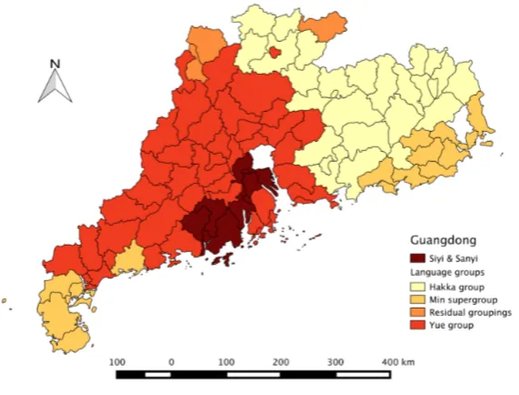
3.3 Distribution of Languages in Guangdong . . . 45

3.4 Distribution of Cantonese Workers Across Sectors . . . 46

A.1 Agricultural Activity in Taiwan 1905 . . . 89

A.2 Correlation between Average and Minimum Rice Prices . 90 A.3 Average Value of Loans and Inputs Provided . . . 91

A.4 Time-varying Treatment Effect Estimates on Log Inputs Provided . . . 92

A.5 Correlation Between Fertiliser Provided and Actual Con-sumption . . . 93

(10)

B.1 Correlation between Workers and Self-employed Work-ers - Downstream Manufacturing . . . 110 B.2 Correlation between Workers and Self-employed

Work-ers - Related Retail . . . 111 B.3 Firm Outcomes: Output, Assets and Capital . . . 112 B.4 Firm Outcomes: Output, Assets and Capital by Export

Status . . . 113 B.5 Firm Outcomes: Employment and Expenses . . . 114 B.6 Firm Outcomes: Employment and Expenses by Export

Status . . . 115 B.7 Economic Census: Effect on Size Distribution -

Manu-facturing . . . 119 B.8 Economic Census: Effect on Revenue per Worker by

(11)

Acknowledgments

First and foremost, I would like to thank my supervisors Rocco

Mac-chiavello and Amrita Dhillon for their guidance and unwavering

sup-port. Their advice and feedback during my PhD has been priceless.

Furthermore, I would like to thank the member of the Department of

Economics for their excellent advice. Particularly, I would like to thank

Sascha Becker, Dan Bernhardt, Clement de Chaisemartin, Natalie Chen,

Nick Crafts, Clement Imbert, Mirko Draca, Bishnu Gupta, Roland

Rath-elot, Debraj Ray, Fabian Walding, Mike Waterson and Chris Woodruff

for taking the time to listen to my ideas and questions. In addition, I

would like to thank the participants at the AMES and CWIP seminar

for their contributions. I would also like to thank Fabrice Defvever for

providing us with data from the Annual Survey of Industries for

Guang-dong province. Gratitude goes to Helen Cao, Winnifred Chu and Kyoko

Oishi for their excellent, and mostly unpaid, research assistance.

I am very grateful for the Initial Training Network, PODER to

allow me to spend one year at the Paris School of Economics. I would

particularly like to thank Denis Cogneau but also Karen Macours and

Akiko Suwa-Eisenmann, as well as the CFDS and PSE-PSI participants

for their valuable feedback. I would also like to thank my office, without

whose directions on all aspects of Paris life I would have been lost.

This thesis would not have been completed without the help and

support of my fellow PhD students, particularly, Adam Hutchinson,

(12)

Raghul Venkatesh. I would also like to thank Boromeus

Wanengkir-tyo for always being happy to stand in when google gave no satisfying

answer. Finally, I would like to thank Anna Baiardi for her constant

emotional and practical support through all the ups and downs, be it as

a friend, flatmate or co-author.

My deepest appreciation goes to my parents and my sister for

their support and love. I cannot thank them enough for giving me the

confidence to pursue my passions knowing that the will always be there

to support me. Lastly, I would like to thank my girlfriend and best

friend, Linda, for her endless supply of courage, motivation and

proof-reading.

Christina Ammon

(13)

Declarations

The second chapter,Farmer Bargaining Power & Relational Contracts in the

Sugar Industry in Colonial Taiwan and the fourth chapterProduct

Customi-sation and Optimal Firm Sizeare solely my own work. The third chapter,

The Benefits of the Bamboo Network in International Trade has been

coau-thored with Anna Baiardi. We contributed in equal parts to the data

preparation and development of the empirical strategy. The results and

the interpretation were developed from joint discussion.

I declare that the material contained in this thesis has not been

used or published before, and has not been submitted for another degree

or at another university.

Christina Ammon

(14)

Abstract

(15)

Abbreviations

ATE Average Treatment Effect

FDI Foreign Direct Investment

GAEZ Global Agro-Ecological Zones

ISIC International Standard Industrial Classification

IT Information Technology

FAO Food and Agriculture Organization of the United Nations

NAICS North American Industry Classification System

NBER National Bureau of Economic Research

OECD Organisation for Economic Co-operation and Development

OLS Ordinary Least Squares

R&D Research and Development

RMB Renminbi

TFP Total Factor Productivity

TFPR Total Factor Productivity Revenue

SIC Standard Industrial Classification

U.K. United Kingdom

U.S. United States

Y Japanese Yen

(16)

Chapter 1 Introduction

Why some countries are poorer than others is one of the most important questions in development economics. The current consensus seems to be that income differences cannot be explained purely by differences in capital and labour, but instead are accounted for to a large extent by differences in total factory productivity, or TFP (Caselli, 2005). At the same time, this difference in aggregate productivity is attributed in part at least to the misallocation of scarce resources. The idea is that mar-ket distortions are causing resources not to be allocated to the firms for which the marginal product is the highest (see for example Hsieh and Klenow (2007) or Restuccia and Rogerson (2013)). Therefore, the study of the constraints and distortions faced by firms in developing countries is key in understanding productivity and hence income differences. It is therefore unsurprising that this topic has sparked a vast literature which investigates how firms are affected by a numerous constraints and distortions in many different settings. The constraints and distor-tions highlighted by this literature range from credit constraints and distorting labour laws to weak institutions (Banerjee and Duflo, 2005, 2012). However, there is still not a clear consensus which factors are the most important in explaining misallocation. This thesis adds to this lit-erature by studying a related question, namely what mechanisms firms and other agents develop in order to (partially) overcome the constraints and distortions they face.

(17)

con-tracts 1, which allow credit to be supplied despite of weak enforcement institutions. I study how sustainable these contracts are to changes of the outside option of one of the parties in the context of the sugar industry in colonial Taiwan. More specifically, I analyse how interlinked lending provided by mills to its suppliers - sugar cane farmers - is affected by a change in the outside option of a subset of the farmers. The outside option is affected by a change in the trend in the price of rice, the main alternative exportable crop. Due to the particular institutional environ-ment, which allocates to each mill a specific fixed area from which it can source cane, I am able to implement a difference-in-difference strat-egy with a continuous treatment intensity according to the suitability of this area for rice cultivation. I digitalise novel historic data regarding lending, production as well as a number of mill level variables. The re-sults indicate that the improvement in the outside option of farmers has a large and significant effect on lending: A one standard deviation in-crease in the suitability for rice is associated with a dein-crease of loans by up to 26%. These results have important policy implications as if these adjustments made by downstream buyers are not taken into account policies that strengthen the bargaining power of small-scale producer could have unanticipated negative effects.

The second chapter, on the other hand, analyses how firms are able to overcome informational and contractual barriers to exporting with the help of ethnic migrant networks in the destination country. More specifically, the chapter considers how firms in southern China that are located in counties that saw a large share of its population em-igrate to the United States in the 19th century (referred to as sending

counties), benefit from their closer relationship to the American-Chinese

population. Access to the network is assumed to vary along two dimen-sions: Firms are assumed to have better access to the American-Chinese network if they are located in one of the original sending countiesandare active in an industry that employs a larger number of ethnic Cantonese in the U.S. This interaction allows us to control for geographic and in-dustry characteristics by including fixed effects. The results show that

1_{Relational contracts are defined as informal contracts that cannot be enforced}

(18)

networks play an economically significant role in facilitating trade both through the extensive and intensive margin. In addition, we find sup-porting evidence that networks predominantly promote trade by lower-ing information barriers.

(19)

Chapter 2 Farmer Bargaining Power &

Relational Contracts in the Sugar

Industry in Colonial Taiwan

2.1 Introduction

Farmers in rural areas of developing countries often do not have access to formal financial institutions. Instead, they rely on other agents in the supply chain for credit, such as intermediary buyers of their products (Hoff and Stiglitz, 1990). Through sustaining relational contracts, these agents are thus able to supply credit profitably despite the weakness of formal contracting institutions. Relational contracts are contracts that are self-enforcing due to the value placed on continuing the relationship i.e. in order to be sustainable, the rents associated with long-term rela-tionships need to be sufficiently large compared to the parties’ outside option. For example, a buyer might be willing to supply credit as the threat of termination of the buyer-seller relationship, which is valued by the farmer, reduces the likelihood of default. Given the prevalence of such informal contracts and their importance for a possible supply of credit, understanding which factors determine the sustainability of these informal contracts is an important question in development (Deb and Suri, 2013).

(20)

mills in Taiwan during the Japanese colonisation (1895-1945). In this setting, the outside option of a subset of sugar cane farmers is the cul-tivation of the main alternative cash-crop, rice. As there were few non-agricultural opportunities, a change in the pay-offs of rice cultivation is likely to be salient. Specifically, I investigate how the reversal in the trend of rice prices in mainland Japan affects sugar cane production through its impact on mill-to-farmer lending and provision of inputs (e.g. fertilisers and seeds).

Rice prices could affect the sustainability of relational contracts in the following way: Consider for example an increase in rice prices. This increase lessens the relative rents associated with maintaining a rela-tionship with sugar mills for the relevant subset of sugar cane farmers. Therefore, the termination such relationships becomes less severe and as such farmers have a greater incentive to default on loans provided by mills. In anticipation, mills will reduce the amount of credit they supply. This reduction in the supply of credit, however, reduces overall farmer welfare. The mechanism described here is similar to the effect highlighted in Macchiavello et al. (2015), who investigate the effect of competition between downstream buyers on relational contracts, which is seen to be significant and negative.

In general, the challenges encountered within the empirical study of factors affecting the sustainability of relational contracts are twofold as not only credible measures of relational contracts have to be recorded, but also exogenous variation in the factors have to be identified. As such, this setting lends itself to studying the effect for a number of reasons. Focusing on only one specific industry allows for the identification of credible measures of relational contract practises. More importantly, the particular cultivation environment required by rice and sugar allow me to implement a difference-in-difference strategy with continuous treat-ment intensity, where the suitability for rice cultivation determines the intensity of treatment by the change in rice prices.

(21)

were only allowed to sell sugarcane to the respective mill. In return, mills committed to purchase all sugarcane grown at a previously an-nounced price. Figure (2.4) shows a map of all command areas in 1918. The command areas were fixed over time and new mills’ areas were re-stricted to land that was not within the command area of another mill. Thus the area from which sugar mills could source cane from was fixed over time. It is important to note that these policies are common across the developing world and is not restricted to sugar cane.

At the same time, fields in Taiwan could be roughly divided into two types: paddy (or wet) fields, which can be sufficiently flooded to grow rice and dry fields with insufficient irrigation for growing rice. Sugarcane however, can be grown both on paddy and dry fields, due to lower irrigation needs.

As the price of rice increased, the outside option of farmers that farmed paddy fields increased, while it remained unchanged for farmers with dry fields. Therefore, keeping the share of paddy fields in each mills catchment area fixed at their 1918 level, I implement the difference-in-difference strategy with continuous treatment intensity according to the field composition of the catchment areas and using both the change

in trendsof rice prices as well as year on year variation. The identifying

assumption is that mills with different shares of paddy fields would have experienced the same time-trend in the absence of treatment.

The information about mill and farmer performance is taken from

theTaiwan Togyo Tokei(1913-1944) (Taiwan Sugar Statistics), which records

yearly statistics about the universe of modern sugar mills during the second half of the colonial period. I digitalise the data for the period of 1929-1939. To my knowledge, I am the first to have digitalised and translated the data to this degree of detail. The main outcomes of in-terest are measures of relational contracts such as lending and provision of inputs by mills to farmers. I further collect data on other farmer and mill outcomes, such as area cultivated with sugarcane, yields, fertiliser use, and information about manufacturing activities.

(22)

fungible loans provided by the mills. On the other hand, I find that the provision of non-fungible inputs remains unchanged. Short run price changes seem to have the opposite effects: a short-run price increase has no effect on monetary lending but increases the inputs provided, which could be indicative of improvements of farmer bargaining position. The result is robust to the inclusion of various control variables as well as prefecture-year fixed effects and mill-level linear trends. I also find no evidence that would lead me to reject the parallel trends assumption.

Further I investigate how other decisions by farmers and mills are affected. I find that the overall area cultivated with sugarcane remains nearly unchanged, though the composition changes. The share of paddy fields is reduced, while the share of dry-fields increases. In addition, I find that though fertiliser usage remains stable, yields are reduced significantly, by nearly 8% overall and by up to 14% for paddy fields. This could be indicative of both adverse incentive effects for farmers but also changes to the field composition. Concerning mill behaviour, I find very little changes except for an increase in the days of inactivity of mills caused possibly by mis-coordination in the harvesting process, which might be indicative of a further breakdown of the mill-farmer relationship.

(23)

to the outside options of farmers. Thus, the main addition of this paper is in allowing the dynamic study of how much and how fast existing informal contracts are affected.

This paper proceeds as follows. Section 2.2 gives historic and contextual background on the Taiwanese sugar industry and Japanese rice policies. Section 2.3 gives a description of the data and section 2.4 outlines the empirical strategy. The results are presented in, section 2.5 and in section 2.6. Finally, section 2.8 concludes.

2.2 Background & Variation in Exposure

2.2.1 The Sugar Industry in Colonial Taiwan

Japanese Colonisation

Previous to Japanese colonisation, Taiwan had been colonised already by both the Spanish and the Dutch in the 17th century, though both nations only controlled a small share of the total territory. Eventually it offi-cially came under Chinese control in 1683 and gained prefecture status in 1887. At the time, Taiwan was characterised by its under-development and lack of rule of law relative to mainland China. After the first Sino-Japanese War in 1895, Taiwan was seceded to Japan under the Ma Kuan Treaty and became a Japanese colony until 1945, when Japan surren-dered unconditionally. The first years of the Japanese colonisation were characterised by fierce resistance by the Taiwanese population against the coloniser and thus Japanese policy was focused on controlling the is-land. After 1915, however, conflicts had essentially ended. The Japanese government then invested heavily in the modernisation of the island including infrastructure, sanitation and schooling (Chou et al., 2007).

(24)

were therefore also imported in certain years.

Sugarcane was the main cash crop and export good in colonial Taiwan. Sugar had been produced in Taiwan since the 16th century, with the knowledge having been brought by immigrants from mainland China. However, both the agricultural as well as the industrial technol-ogy remained essentially unchanged until the arrival of the Japanese colonialists, which invested heavily to modernise the industry. The traditional production technique was characterised by low yields, high labour intensity and the production of low quality product. While some larger mills existed, which were able to produce white sugar, the ma-jority of mills were very small and produced brown sugar for domestic consumption. Before the arrival of the Japanese colonisers, Taiwan was thus far behind the world frontier: while Java and Hawaii, the most productive sugar producers in the 19th century, produced 30-34 tons of cane per acre, Taiwan produced merely 12 (Davidson, 1903). Even before colonisation, the main export destination for sugar was Japan. Farmers operated under share-cropping agreements and were able to obtain lim-ited loans from sugar merchants. Even under this system farmers were supposed to sell their cane to their lender, however, there was free com-petition between lenders and there was no formal enforcement mecha-nism of this rule. Hence, unsurprisingly, defaults were common, leading to credit rationing and high interest rates (?).

(25)

to sell to that specific mill. Further farmers were not allowed to trans-port cane across Prefecture borders. On the other hand, mills had to announce a purchasing price for the cane before planting took place, i.e. around one and a half years before harvests. These prices were recorded centrally and published in an industry publication. Mills then had to commit to purchase all cane produced within their command area for the announced price (Ka, 1991). In order to ensure sufficient supplies, mills were providing fertiliser, seeds and other loans. The interest rate for these loans had to be announced at the same time with cane prices before the first planting i.e. 18 months in advance and published cen-trally, making it easier for farmers to enforce prices. Mills however were allowed to and did often price discriminate and charged differentially for paddy and dry fields, but also paid higher prices per ton to farmers with more productive fields (Koo and Wang, 1999).

Under these measures, the sugar industry developed successfully. By 1910, 29 modern mills had been founded, a number that rose to 45 by 1939. With the outbreak of World War II, the sugar industry became strategically important, as one of the side products of sugar production, molasses, could be used for ethanol production, which in turn was used to power various war machinery. Thus the industry became much more regulated and production targets were set centrally.

2.2.2 Sugar Production

All sugar production follows the same basic principle: sugarcane is first crushed, and a sucrose-rich juice is extracted. Afterwards the juice is cleansed of impurities, then reduced through boiling and finally the mo-lasses are separated from the sugar crystals. However, each step of the process can be mechanised to a differential degree. Mechanisation, such as mechanical cutters, vacuum pans and centrifuges, does not only lower marginal costs, but equally importantly increases the quality of sugar.

(26)

could be processed at any given time. In addition, preventing machine breakdowns and organising swift repairs can influence efficiency signif-icantly, as otherwise the cane at the mill will start to deteriorate. For a more detailed discussion of sugar production see Sukhtankar (2016).

The growing period of sugar varies according to the climate it is grown in: in the tropical south of Taiwan, the growth period is around one year, while it averaged around 18 months in the sub-tropic north. The crop is water- and fertiliser intensive, however in Colonial Taiwan it was traditionally mostly rain-fed. Fertiliser, which was previously rarely used, as well as new seed varieties were subsidised by the Japanese Governor General. The harvesting period in Taiwan started between December and continued until May. In the tropical south in principle cane can be grown during the entire year; however, possibly due to irri-gation needs, this was not done during the period. The quality of cane is predominantly defined by its sucrose content, which causes mills and farmers to have opposing incentives regarding the optimal harvesting period: While later harvesting leads to a higher sucrose content, it also implies lighter and dryer cane. Since prices are paid to the farmer per ton of cane, drier cane implies a lower income to the farmer (Koo and Wang, 1999).

2.2.3 Rice Cultivation and Agricultural Rice Policy in Japan

Japanese rice prices experienced a period of extreme volatility from 1910-1940, which is characterised by a number of trends caused by economic policy interventions into the rice market in Japan.

(27)

suc-ceeded in 1925. Similar schemes were under way in Korea, which was the dominant source of rice for the Japanese market.

Due to the expansion in the rice production capacity from the 1920s onwards, the rice price started to decrease dramatically form 1925. This was partly due to the increased production in the colonies, partic-ularly in Korea, but also in Taiwan. However, domestic production had also increased significantly. Coupled with the economic recession after 1929, the overproduction lead to collapse of prices. In 1930, the price of rice fell by up to 30%, leading to unrest of rice farmers in Japan. The Japanese government responded through several measures between 1931 and 1933. In 1931, a revision of the rice law was passed, which stated that the state would put upper and lower bounds on the price of rice and further subsidised rice storage. Furthermore, in 1932 the government quite suddenly committed to unlimited rice purchases, and further expanded the purchasing schemes in 1933. At the same time, with the military actions in Manchuria in 1931, the demand for rice in-creased independently (Sheingate, 2003). As a result the trend of rice prices was reversed and prices continued to increase until the outbreak of World War II.

[] Overall, the Japanese rice prices followed rice prices in most South-East Asian countries until the early 1920s, when all countries ex-perienced a spike in their prices. However, the Japanese reaction to the price spike of aggressively increasing production, changed the price tra-jectory in the Japanese market. While Japanese prices started to decrease dramatically from 1925 onwards, most other countries in the region ex-perienced a continuous increase in prices until 1930. This increase how-ever, was reversed dramatically in 1931 when rice prices in many coun-tries nearly halved. This was due to the Depression in general, as well as protectionist policies among others in Japan in particular. Japan was one of the largest markets and importers of rice in the 1920s and there-fore the trade restrictions heavily affected rice prices in its neighbouring countries. Table A.2 shows the prices for the example of Thailand. Prices in the region slightly recovered until the end of the 1930s, however never came close to the 1920 levels (Boomgaard and Brown, 2000).

(28)

the heavy protectionism Japan imposed as well as the aggressive inter-ventions in the rice market. Rice prices fell earlier than in most other countries due to the development of overproduction in Japan and its colonies, and were increasing and not falling in the 1930s due to the extensive purchasing scheme imposed by the government, which pur-chased sufficient rice to positively affect prices. []

2.3 Data and Descriptive Statistics

In this section, I give a brief overview of the most important datasets and the main variables of interest as well as some summary statistics.

2.3.1 Outcome Variables

Data on Lending and Input Provision

The data on lending and the provision of inputs by mills to farmers is digitalised from the Taiwan Togyo Tokei (1913-1944) (referred to as Tai-wan Sugar Statistics). The data was self-reported by the factories and published annually at the mill level. The Taiwan Sugar Statistics was published by the Governor Generals Office from 1913 until 1944. Infor-mation on lending and similar activities, however, only becomes avail-able from 1929 onwards. Furthermore, I exclude data after the outbreak of World War II, as not only did the Japanese intervene more forcefully in the market during this period, but also sugar factories were targeted by allied bombing during the later stages of the war. Thus, I focus on the period of 1929 to 1939.

(29)

As mills are identified by name, I am able to construct an unbal-anced panel of 45 modern mills. As the the empirical strategy applied requires that firms exist already in 1918. This leaves me with 35 mills that were founded before 1918 and exist until 1939. Table A.3 lists all of the modern mills active over our period of interest and whether the firm is in our sample, as well as its ownership, age, capacity and share of paddy fields of the total catchment area.

Loans are recorded in Japanese Yen and include both loans made for working capital as well as miscellaneous (consumption) loans. Fur-thermore, loans made in kind for inputs are also recorded in Yen value and include the provision of fertiliser and seeds. One outcome variable is the log total value of loans by type provided. However, a decrease in the total value of loans provided could not only be caused by a decrease of supply by the mills due to the decreased willingness to lend, but it could derease mechanically if the area cultivated with sugarcane de-creases and thus the number of sugar cane farmers is decreased. Thus, I also create an adjusted loan(Loansg _i_,_t) variable for each type of lending

or input provision activity, which is normalised by the area cultivated with sugarcane within each mill’s command area at a given time t in the following way:

g

Loansi,t = Loansi,t/area sugarcanei,t (2.1)

Figure 2.1 depicts the density of the normalised total value of all loans and inputs provided in the year 1930. It is clear that there is large variation of the amount of inputs and loans provided by mills. The total value per hectare farmed with sugarcane ranges from around 90Yto up to over 450Y, with a mean and median of 234.7Yand 212.3Yrespectively. Figure 2.2 shows the evolution of the four types of loans over time. Working Capital and Fertilizer make up the biggest share of total loans. What is noticeable is that both experience a strong drop previous to 1931, but while fertilizer provision rebounds strongly, working capital only reaches pre-1931 levels late in the 1930s. Overall, however, there seems to be an upward trend in the provision of credit during the 1930s, possibly as the industry was maturing.

(30)

pro-Figure 2.1: Density of Total Value of Loans and Inputs per Hectare Farmed

vided is not completely obvious. In addition to overall effects of the fi-nancial crisis, which might have decreased the liquidity of the Japanese parent companies, i t has been documented historically, that the sugar industry in Taiwan suffered severely during the early thirties, due to the fall in sugar prices in Japan (Fan, 1967). As can be seen in Figure 2.3, the total amount of loans tracks the sugar price quite closely. As sugar prices fell, investment in sugar becomes less profitable from the point of view of the mills and therefore they might have had less incentive to supply costly credit.

[]

Mill and Farmer Data

[image:30.595.128.496.96.366.2]

(31)

[image:31.595.118.497.100.377.2]

Figure 2.2: Loans by Type over Time

18

20

22

24

26

Su

g

a

r

Pri

ce

s

100

150

200

250

300

L

o

a

n

s

to

F

a

rme

rs

1930 1935 1940 1945

year

Loans to Farmers Sugar Prices

[image:31.595.113.487.407.682.2]

(32)

by the type of field. It is important to note, that this data was reported by the mills and thus is aggregated at the mill level. Concerning the mills, I have information on the area planted with sugarcane by the mills distinguishing between paddy and dry fields and the respective yields. From this I calculate what percentage of total paddy fields or dry fields is being cultivated. Furthermore, I have information on sugar production: In addition to detailed information on sugarcane used and the amount of sugar produced, I have also a measure of technical efficiency - referred to as the sugar yield- that takes into account the quality of sugar produced. Further, I have detailed information on capital investment as well as information about the length of the harvest as well as how many days the factory was inactive during this period. The latter is of particular interest, as it is very costly for the factory to be inactive but at the same time reducing this time relies heavily on a close cooperation between farmers and mill. I further digitalised a number of variables to be used as controls, such as the equity level of the parent company in 1918, the size of the parent company in terms of number of factories, the total size of the command area as well as mill age. Unfortunately, I have no information on labour employed. It should be noted, however, that if mechanised production methods are used, labour costs are a small share of total costs in sugar milling. Table 2.1 gives the relevant summary statistics.

Finally, I also include a number of controls on the prefecture level: prefecture population, total cultivated land and per capita ownership of livestock.

2.3.2 Measures of Exposure to Rice Price Changes

The key variation of the empirical strategy is the degree to which mills and the farmers in their command area are affected by changes in the outside option of the farmers due to changes of rice prices in Japan. The effect of rice prices on the average farmer outside option is assumed to be a function of the average suitability of the command area for the cul-tivation of rice. Thus the measure of treatment intensity is the averarge rice suitability of each mill’s command area.

(33)

Variable Observation Mean Std. Dev Min Max Command Areas

Share of Paddy Fields 391 .437 .298 0 .998

Command Area (h) 391 117349.8 708380.7 3866.285 4726422 Farmer Outcomes

Fertilizer (jin)

Share of Paddy Fields - Farmers (%) 303 66.8 5.4 0 79.5 Farmer Paddy Fields Yield (Jin/h) 470 126.418 161.228 11.941 3558.427 Share of Dry Fields - Farmers (%) 312 20.8 10.2 3.3 77.8 Farmer Paddy Fields Yield (Jin/h) 469 119.1 28.7 11.9 237.9 Farmer Dry Fields Yield (Jin/h) 496 97.4 25.7 31.4 169.8

Mill Outcomes

Share of Paddy Fields - Mills (%) 342 9.1 3.53 0 44.4

Share of Dry Fields - Mills (%) 338 6.8 8.7 0 56.2

Mills Paddy Fields Yield (Jin/h) 496 130.5 37.4 34.7 258.2 Mills Dry Fields Yield (Jin/h) 496 113.4 40.3 18.19 364.1

Cane Used for Production (tons) 481 236.5 176.8 223.4 978.4

Sugar Output (tons) 482 30.6 22.5 0.7 121.4

Sugar Yield (%) 482 12.1 2.5 5.5 15.5

Capital (tons)

Harvest Duration (days) 482 133.8 31.6 50 240

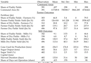
[image:33.595.115.495.100.361.2]

Share of Days not Operation (share) 479 .415 .378 0 .98 No. of mills: 38

Table 2.1: Summary Statistics

determinant in whether a given field is suitable for rice cultivation, as the field needs to be flooded at the beginning of the growth cycle of rice. Fields that can be naturally or artificially flooded thus are referred to as paddy fields. The Japanese colonial administration distinguished thus between three types of fields: Paddy fields that are rain-fed, which means that they are only sufficiently irrigated for rice plantation once a year, paddy fields that are linked to man-made irrigation channels and thus can be cultivated twice a year and finally so-calleddry fieldsthat are not suitable for rice production. Sugarcane on the other hand requires less intense irrigation and thus can be grown on all three types of fields 1_.

For certain years, the Taiwan Sugar Statistics contains information on the area within each command area that is of either of the three types and that is also suitable for the cultivation of sugarcane. Thus, as one of my measures of rice suitability, I calculate the share of the total land suitable for sugarcane cultivation within the command area that

1_{While sugarcane is an irrigation intensive crop, it does not however require as}

(34)

are paddy fields i.e. the area within the command area that are paddy fields and suitable for sugarcane divided by the total land suitable for sugarcane:

suitability_ipaddy_,_t = paddyi,t/total landi (2.2)

Note that while the total land within a command area is fixed over time, as the border of command areas remained unchanged, the area of fields that are paddy fields could and does indeed change over time due to improvements in the irrigation system. This causes an endogeneity is-sue, as mills that gain better access to irrigation might be fundamentally different from those that do not, and thus these unobservable charac-teristics might be driving the results. Thus, I restrict the area of paddy fields at its 1918 level, the earliest year for which the information is made available. As a result, the suitability becomes a time-invariant variable. This restricts the sample to mills that have been active since 1918 and are still active in 1930.

suitability_ipaddy = paddyi,1918/total landi (2.3)

As a further robustness check, in some specifications, I restrict the measure of suitability to the share of land that are only rain-fed paddy fields and exclude all artificially irrigated fields, i.e.

suitabilityrain_i −f ed =rain-fedi,1918/total landi (2.4)

In some occasions, I further use the rice suitability measure from the Food and Agricultural Organization (2016) crop-suitability data. Specif-ically, I use the land-suitability for wetland rice using low-level inputs, i.e. assuming no man-made irrigation is available, again to avoid en-dogeneity concerns. I calculate the treatment intensity variable using information about the exact GIS coordinates of the boundaries of each mills command area in 1918. While this measure is less subject to en-dogeneity concerns, it is also likely to be less exact as the earliest point measured is 1962. Thus, in most specification, I use the measures based on the Japanese data.

(35)

(a) Cane Suitability (b) Rice Suitability

Figure 2.4: Command Areas by Crop Suitability

Notes: Maps are based on the FAO crop suitability index, which ranges from 1 to 9. GIS Data on the boundaries of the command areas has been compiled by the Academia Sinica’s Institute. Higher suitability is indicated by darker colouring.

areas, using the FAO measure. It is clear to see that rice suitability is not randomly distributed: mills in the north have command areas that area significantly more suitable for rice cultivation than in the south. The suitability for sugar cane follows the opposite pattern as shown in Figure 2.4a. This gives rise to concerns that mills in the north are fundamen-tally different from those in the south and thus would have developed differently independent from the treatment. Further discussion of these concerns and what I do to address them follows in Section 2.4.3.

2.3.3 Prices of Rice, Sugar and Other Agricultural Goods

The price data for the agricultural products is taken from Japanese and not from Taiwanese markets, in order to avoid reverse causality concerns i.e. to rule out that price data is influenced by changes in the supply and demand of farmers and mills.

(36)

While changes to rice prices affect the outside option of paddy farmers, it does not take into account possible changes to the outside option of dry field farmers. Thus, similarly to before, I proxy changes to the outside option of dry farmers with the changes to the price of the main crop produced on dry fields, namely red and black beans. Bean prices are also reported in yen per Koku at the Tokyo market. The data is taken from the Taiwan Statistical Yearbooks (1922-1939) that were compiled by the Taiwanese Governor General’s office, under the Japanese administration. They are reported annually and distinguish between red and black bean prices. I take a simple average of the two prices. In my analysis, I then focus only on changes to the relative price, which is the rice prices divided by the average bean price.

Information on the sugar prices are taken from the Taiwan Sugar Statistics, which records monthly prices for refined sugar on the Tokyo market. Prices are measured in yen per 100 jin (60kg) from 1918 until 1944. I calculate a yearly average in order to correspond to rice prices.

Figure 2.5 shows the evolution of all three prices over time. There is a clear downward trend for rice until 1931, indicated by the second dotted line. After 1931, the price begins to rise steeply. The first dotted line indicates the introduction of Ponlai rice in Taiwan, only after which the shown rice prices became salient for Taiwanese farmers. While both sugar and beans also reach their lowest point in 1931, they do not ex-perience the same dramatic reversal as rice. Sugar prices, in particular, decrease until 1931 but remain relatively low thereafter.

2.4 Empirical Strategy

(37)

[image:37.595.129.499.101.368.2]

Figure 2.5: Agricultural Goods Prices on Japanese Mainland

Sugar and Bean prices are prices are measured in Tokyo while rice prices are measured in Osaka. Refined sugar price: 1 yen purchases 100 jin (60kg). Rice & Bean prices: one yen purchases one Koku (278.3 litres). Ponlai rice was available for cultivation in Taiwan only from 1925 onwards, as indicated by the first dashed line. The second dashed line indicates the timing of the change in rice policy on the Japanese mainland. 1 Japaneses Yen was equivalent of 0.5 USD at the time.

2.4.1 Patterns of Firm Characteristics and Rice Suitability

As can be seen in Figure 2.4b, command areas that are larger and further in the north have a larger share of paddy fields. This indicates that rice suitability is not allocated as if random, which might also imply that the common trend assumption could be violated.

(38)

that a higher share of paddy fields is associated with a later year of es-tablishment,though it disappears somewhat once prefecture fixed effects are included. This negative correlation between age and paddy share is supported by the historical literature. It is seen to be a consequence of the exclusive command area legislation, which implied that new mills could only be founded on land that was not yet within the command area of another mill. Therefore, older mills had an advantage in estab-lishing themselves in their preferred location, which are usually in the dryer south that is more suitable for sugar cane cultivation. The results for the variables regarding the parent company are more surprising, as they indicate that larger companies are more likely to establish a mill in a location with paddy fields.

Share of Paddy Fields of Total Area

(1) (2) (3) (4)

Year of Establishment .026** .033*** .019 .013 (.011) (.011) (.014) (.016) Size of Command Area (100 000h) .010*** .014*** .014***

(.001) (.002) (0.02) Number of Factories owned by Company .015 .013** -.018 (.011) (.006) (.027) Company Equity in 1918 (million Yen ) .007

.007

Prefecture FE N N Y Y

R2 _.10 _.23 _.53 _.65

[image:38.595.113.497.328.528.2]

N 35 33 33 33

Table 2.2: Mill Characteristics that Predict Paddy Share

Robust standard errrors are in parantheses.***p>0.001 **p>0.05 *p>0.10

I then plot the main outcome variable, total monetary loans pro-vided, on the residual from column (4). Figure 2.6 shows that reassur-ingly there is little correlation.

2.4.2 Difference-in-Difference Estimation

(39)

[image:39.595.125.500.104.367.2]

Figure 2.6: Correlation Between Residual Paddy Share and Log Total Monetary Loans

period t on the expectedrice price in period t+1 and t+2. Thus, unex-pected shocks to rice prices should only have a small impact (assuming all agents are rational). Instead, they should adapt their behaviour pri-marily if the change is assumed to be permanent or the trend in prices are changing. As outlined in section 2.2.3, in 1931 there were a num-ber of policies that could be reasonably expected to change the level and also possibly the trend of rice prices for the future. Figure 2.5 shows that indeed the rice price experiences a dramatic change in terms of trend. Thus, in my main specification, I analyse the change of lending before and after 1931 in a difference-in-difference estimation strategy with con-tinuous treatment intensity.

[] To highlight this point, one could consider the incentive con-straint in a simple credit model of strategic default with a single model as is proposed in (Ghosh et al., 2000). Suppose that there is a single lender, which in this case is the mill. There are three periods: In period t-1, the mill announces a contract consisting of Lt, which is the loan it

(40)

payment for the sugarcane sold by the farmers. Farmers observe this contract and in period t decide whether to plant sugarcane or rice. For simplicity assume that this is a binary decision. The planting decision is an essence already a decision on whether the farmer wants to default on the loan: If the farmer plants sugarcane, he or she is forced to repay the loan, as the mill is a monopolist and will simply deduct the loan repayment, i.e. if the farmer decides to plant sugarcane, in period t+1 he or she harvests the cane and sells it to the monopolist, foryc_t −(1+r)Lt.

If the farmer, however, has taken out a loan and decides to plant rice, the mill imposes a large fine. Therefore, repayment is likely to be impossible or not desirable. Therefore, if the farmer has planted rice, in period t+1, he or she will default on the loan. In this case, the farmer earns income yr_t form his or her rice harvest. Suppose that yr_t < yc_t The time line can also be seen below:

Figure 2.7: Timeline

In the case of default, the mill historically imposed heavy fines, which I assume in this case implies that the farmer is no longer able to either borrow from nor sell to the mill and therefore is no longer able to produce sugarcane. Supposing that the farmer has a discount factor of δ, it can be shown easily that the farmer only repays his or her loan if the following incentive constraint is satisfied:

IC:

∞

∑

t=0 δt

Etyct

−(1+r)L ≥

∞

∑

t=0 δt

Etyrt

+L (2.5)

(41)

is more likely to bind if expectations about future rice prices are higher keeping cane prices fixed. In this way contemporaneous prices should only matter for informing expectations about future prices. This is in part, because decisions about defaulting are made at the planting stage and therefore by design future prices are the relevant statistic and in part due to the fact that by defaulting the farmer closes off the possibility of selling sugarcane to the mill in the future. The latter means that while the first period’s prices are important, expectations about theprice trend are even more important for the decision. As a result, the empirical strategy will primarily focus on the change in trends, though I also use contemporaneous prices in some specifications []

As variables are reported at the mill level, the treatment intensity varies also at the mill level and depends on the share of fields within a command area of the mill that are suitable for rice production. In my baseline specifications this is measured as the area of paddy fields as a share of the total area within the command area that are suitable for sugarcane cultivation, as outlined in equation 2.3.

The panel data structure of the data allows me to include both year and mill-level fixed effects, which implies that all unobserved time invariant mill and farmer characteristics, as well as any year effects that are common across all mills are absorbed. However, imbalances between factories with a high and low paddy share could be associated with dif-ferential time trends. As most paddy fields are in the north of Taiwan, the two samples are indeed not balanced. Thus, I further include prefec-ture specific time trends. In addition, I include time-varying prefecprefec-ture controls to capture non-linear trends, such the population working in agriculture, the total cultivated land in the prefecture and the number of cattle per capita as a proxy for rural incomes.

(42)

final specification therefore becomes:

yi,t=α0+α1postt·paddyi+θi+γt+pre f ecturep·t+agei,t+Xi·posti+εi,t (2.6) whereyi,t are the factory-level outcomes at time t, θi and γt are the

fac-tory and time fixed effects respectively, and pre f ecturec·t are the region

specific time trends. agei,t denotes the age of mill i at time t, andXi are

time-invariant mill controls The main variable of interest is the interac-tion of postt, a dummy that equals 0 at time t ≤ 1931 and equal to 1

otherwise and paddyi, the share of paddy fields of total area suitable for

sugarcane cultivation within the command area of a given mill measured in 1918. The effect thus represents the average change in lending across all time periods after 1931 proportional to the share of paddy fields.

The main regression analyses the effect on the value of loans dis-pensed and inputs provided. However, a decrease in total value might simply be caused by a reduction in the amount of sugarcane being cul-tivated. Thus the main variable of interest is the value of loans (and inputs provided) in Yen normalised by the area in hectares that is used for sugarcane cultivation in the same year. While this does not exclude that the effects observed are caused by a reduction in demand, it does rule out the purely mechanical channel of reduced production that could be driving a possible reduction in lending.

Trend break vs. Price Changes

The empirical strategy outlined in the previous section, concentrates on the the break in trends of rice prices, and not primarily on the actual price in each period. This is due to the fact t

2.4.3 Identification concerns

(43)

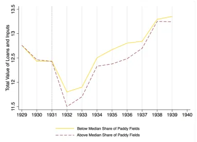
One way of addressing this concern is to check whether mills with different treatment degrees exhibit parallel trends before the treatment takes place. This is somewhat challenging for the main variables of in-terest, lending and the provision of inputs, as these are recorded the earliest in 1929. Therefore, there are just two time periods before 1931, the year price trends changed. Figure 2.8 shows the average total value of all loans as well as of the inputs provided over time split up for mills with a higher or lower than median share of paddy fields. Note that given that rice prices are not constant before 1931, we do not necessarily expect the pre-trends of the two groups to be perfectly parallel. It would be important however, that the pre-trends are not such that they con-tribute in explaining the treatment effect we observe. Figure 2.8 shows that, in the two periods before treatment, 1929 and 1930, the two groups experiencing a near identical trend. Figure A.3 shows the same trends for loans and for the two inputs, seeds and fertiliser, separately. Again, pre-1931, the trends seem very similar. Though this is reassuring, it is important to note the two periods may not be sufficient in order to establish a parallel trend.

(44)

[image:44.595.115.499.97.374.2]

Figure 2.8: Average of Log of Total Value of Loans and Inputs Provided

The total value of loans and inputs for mills with less than median share of paddy fields is normalised to equal those of mills with above median share in the year 1929. Values are expressed in loged Yen.

2.5 Results on Lending

2.5.1 Baseline Results

(45)

represent around 11% of the average value of loans and inputs pro-vided. Column (3) includes further time-varying prefecture controls as well as time-invariant mill controls interacted with a post-1931 dummy. The coefficients remain nearly unchanged; however, the sample size is somewhat reduced due to missing values for some of the mill control variables. Column (4) to (7) show that the decrease is clearly driven by a decrease in monetary loans. Column (4) and (5) show that a one stan-dard deviation increase of paddy fields causes loans to fall by 25.6 Y per hectare, which increases to 26.8 Y per hectare when mill and prefec-ture controls are included. Given that average value of loans provided is around 103Y/hectare, this constitutes a fall of over 26%. Inputs pro-vided by the mills of the farmers, however, remain unchanged as can be seen in columns (6) and (7). Table A.4 conducts the same exercises using the logged value of the same outcomes as in Table 2.3. While the mag-nitude of the coefficients represent a slightly larger percentage change, they are less precisely estimated and lose significance, when the full set of controls are used. Table A.6 goes further in splitting loans according to type, which support the findings in Table 2.3.

The results of the baseline specification are consistent with a de-crease in the sustainability of relational contracts between mills and farmers. The fact that the effect is driven exclusively by the decrease in fungible loans and that non-fungible inputs are nearly unchanged sup-ports the hypothesis that this effect is driven by the increase by farmers’ incentive to default. If the effect was purely caused by a decrease in field quality used for can cultivation or a decrease in demand for cane related inputs, there should be a similar negative effect on the provision of in-puts. However, compositional effects may well play an important role as more credit worthy farmers might have switched to rice production.

(46)

in Table A.5. While the effect on total loans per hectare cultivated with cane looses its significance, the results for monetary loans remain robust.

Total Lending & Inputs Monetary Loans Inputs Provided

Y/hectare Y/hectare Y/hectare

(1) (2) (3) (4) (5) (6) (7)

post* paddy -18.923** -24.420** -24.662** -25.593*** -26.828*** 1.201 2.739 ( 8.094) (11.983 ) (10.799) (9.200) (7.691) (4.696) (5.191)

post 19.153

(12.879) paddy 153.097***

(48.561)

Factory FE N Y Y Y Y Y Y

Year FE N Y Y Y Y Y Y

Prefecture Trends N Y Y Y Y Y Y

Prefecture Controls N N Y N Y N Y

Mill Controls N N Y N Y N Y

N Mills 38 38 33 38 33 38 33

N Observations 360 360 291 360 291 360 291

R2 _.014 _.853 _.860 _.837 _.824 _.802 _.816

[image:46.595.115.496.148.382.2]

Mean 209.74 209.74 209.74 102.93 102.93 106.89 106.89

Table 2.3: Loans and Inputs Provided Per Hectare Cultivated with Cane

Notes:The dependent variables are expressed as the total amount divided by the area on which sugarcane is being cultivated in the same year. The independent variable has been normalised such that one unit equals one standard deviation. Prefecture con-trols include prefecture population, the population employed in agriculture, number of cattle owned and total land under cultivation. Mill controls are age as well as parent company equity, the number of factories owned by the parent company and total size of the command area, which are all interacted with a post-1931 dummy. All standard errors are clustered at the factory level. ***p>0.001 **p>0.05 *p>0.10

(47)

effect on lending, but instead the change in trends, as captured by the post-1931 dummy, has a significant negative effect. The opposite is true for the inputs provided. Here, the short run price shocks seem to have a positive effect on the value provided per hectare. This again could be caused by the improved bargaining position of farmers or mills trying to compensate for the decrease of fields cultivated with sugarcane.

Total Lending & Inputs Monetary Loans Inputs Provided

(1) (2) (3) (4) (5) (6)

pricet−1∗paddy -3.380 11.328 -12.351** 2.131 9.306*** 10.611** ( 7.678) (10.162 ) (5.718) ( 6.811) (3.520) (4.282)

post∗paddy -29.737** -27.891** -2.516

(12.408) (9.336) (5.817)

Factory FE Y Y Y Y Y Y

Year FE Y Y Y Y Y Y

Prefecture Trends Y Y Y Y Y Y

Prefecture Controls Y Y Y Y Y Y

Mill Controls Y Y Y Y Y y

N Mills 38 33 33 33 33 33

N Observations 291 291 291 291 291 291

R2 .854 .861 .811 .823 .819 .820

Mean 209.74 209.74 102.93 102.93 106.89 106.89

Table 2.4: Baseline Specification Including both Prices and Post-1931 Dummy

2.5.2 Robustness

(48)

fixed effects as well as mill-specific linear trends. Secondly, I allow for non-linear effects.

Table A.8 shows the results on fungible lending when prefecture-year fixed effects and linear mill trends are included. Prefecture-prefecture-year fixed effects capture all the variation that is caused by non-linear pre-fecture specific trends. Including linear mill time-trends means that our coefficients no longer capture any linear changes at the mill level over time. Columns (2) and (3) display the effects for the prefecture-year fixed effects, first without and then with mill controls. The negative effect on lending remains robust and the magnitude of the coefficients also re-mains similar. Columns (4) shows the coefficients for the baseline equa-tion is augmented for linear mill time-trends, and Column (5) shows the same when prefecture controls are included. Again, the results remain robust.

The results for the non-linear effects specification are shown in Table A.9 as well as in Figures 2.9 and A.4. As mentioned above, un-fortunately, lending data is only recorded for two time periods prior to treatment and thus there is a limit how informative this is about the pre-trends. Due to missing values for the area farmed in 1929, here the log total values are shown. Reassuringly, Figure 2.9 and Table A.9 show that the negative effect of treatment on lending only sets in after 1931.

(49)

[image:49.595.125.498.106.370.2]

Figure 2.9: Time-varying Treatment Effect Estimates on Log Loans (mon-etary)

Notes: The outcome variable is the log value of all monetary loans. Confidence inter-vals shown are at the 99%, 95%, 90% and 80% levels. The reference year is 1931.

2.6 Other Outcomes

In this section, I present the effects of the change in rice price trends on other behaviours of farmers and mills.

2.6.1 Farmer Outcomes

The outcome variables concerning farmer behaviour are firstly the area cultivated with sugarcane, the use of fertiliser and subsequent yields of fields farmed.

(50)

de-Total Lending & Inputs Monetary Loans Inputs Provided

(1) (2) (3) (4) (5) (6)

post* paddy -11.651 -13.955** -10.950** -14.396*** -.564 .613 (7.243) (7.040) (5.468) (4.450) (3.961) (4.632)

Year FE Y Y Y Y Y Y

Prefecture Controls N Y N Y N Y

Mill Controls N Y N Y N Y

N Mills 38 33 38 33 38 33

N Observations 360 291 360 291 360 291

R2 _.841 _.829 _.830 _.815 _.772 _.816

Mean 209.74 209.74 102.93 102.93 106.89 106.89

Table 2.5: Baseline Results Using Rain-Fed Paddy Fields Only

crease in the total area. When splitting the regression by type of field, we see that there is a large and highly significant decrease of paddy fields that are used for sugar cultivation of between 47-51% (see Column (3) and (4)). Column (5) and (6) show that this decrease is offset by an increase in dry fields on which sugarcane is grown of between 12.5% and 21.5%. While these effects are not very surprising, they do however give support to the hypotheses that the post-1931 captures only an effect related to rice prices, as it affects the two types of fields such an asym-metric way.It is also important to note that the results do not simply indicate the straight forward propositions that a permanent increase in rice prices decreases the area cultivated with sugarcane, but instead that this increase decreases sugarcane cultivation more than proportionally in areas with a larger share of paddy fields.

(51)

presump-tion that the fertiliser provided is non-fungible and thus it should be employed for cane cultivation. Figure A.5 shows the correlation between fertiliser provided and fertiliser consumption. The correlation is around 1.111 and very strong. Indeed there are only few observations clearly below the 45 degree line. Note that we would expect that the actual fer-tiliser consumption should be larger than what was provided from the mills, as fertiliser consumption also includes traditional fertilisers, such as animal manure. The effect on fertiliser consumption are displayed in Table 2.6. Column (1) and (2) show the effect on the logged value in Yen, which is virtually unchanged by treatment. Further, column (3) and (4) show the effect on the fertiliser used per hectare cultivated with sugar-cane in the same year. Again there is no significant effect. Finally, in column (5) and (6), I investigate whether the treatment has an effect on fertiliser consumption relative to the value provided by the mills. A neg-ative coefficient could for example imply that farmers divert provided fertilisers to other crops, or would decrease their spending on additional fertiliser. However, again the coefficients are insignificant.

The final farmer outcome are sugarcane yields shown in Table A.11. Column (1) and (2) show the effect on all field types, while the subsequent columns distinguish between paddy and dry fields. The treatment effect is negative overall, which however could have been ex-plained by the change in the share of paddy fields of the area being cultivated with sugarcane, given that the yield of paddy fields is signif-icantly higher than for dry fields. When running separate regressions for each type of field, it can be seen that the negative effect existswithin both field categories. This could be due to decreased yield per field or instead due to compositional changes of fields, due to both the increased outside option but also possibly due to the lower provision of credit by the mills. Unfortunately, I do not have field level information and thus cannot distinguish these two channels.

2.6.2 Mill Outcomes

(52)

produc-Fertiliser

Log Total Value Y/hectare Actual Usage/Provision

(1) (2) (3) (4) (5) (6)

post* paddy -.007 -.005 3.189 2.382 -.094 -.067 (.068) (.073) (6.529) (5.206) (.090) (.049)

Year FE Y Y Y Y Y Y

Prefecture Controls N Y N Y N Y

Mill Controls N Y N Y N Y

N Mills 42 33 42 33 42 33

N Observations 360 360 291 360 291 291

R2 _.841 _.829 _.830 _.815 _.772 _.816

Mean (piculs) 251827.3 114.468 1.643

Table 2.6: Effect on Fertiliser Consumption

Notes:In the last two columns the dependent variable is divided by the value of inputs provided by the mill. The independent variable has been normalised such that one unit equals one standard deviation. prefecture controls include prefecture population, the population employed in agriculture, number of cattle owned and total land under cultivation. Mill controls are age as well as parent company equity, the number of factories owned by the parent company and total size of the command area, which are all interacted with a post-1931 dummy. All standard errors are clustered at the factory level. ***p>0.001 **p>0.05 *p>0.10

Essays in development economics

warwick.ac.uk/lib-publications

Essays in Development Economics

Kerstin Christina Ammon

Thesis

Doctor of Philosophy

in Economics

Department of Economics

Contents

List of Tables

List of Figures

Acknowledgments

Declarations

Abstract

Abbreviations

Chapter 1

Introduction

Chapter 2

Farmer Bargaining Power &

Relational Contracts in the Sugar

Industry in Colonial Taiwan

2.1

Introduction

2.2

Background & Variation in Exposure

2.2.1

The Sugar Industry in Colonial Taiwan

2.2.2

Sugar Production

2.2.3

Rice Cultivation and Agricultural Rice Policy in Japan

2.3

Data and Descriptive Statistics

2.3.1

Outcome Variables

2.3.2

Measures of Exposure to Rice Price Changes

2.3.3

Prices of Rice, Sugar and Other Agricultural Goods

2.4

Empirical Strategy

2.4.1

Patterns of Firm Characteristics and Rice Suitability

2.4.2

Difference-in-Difference Estimation

∑

∑

2.4.3

Identification concerns

2.5

Results on Lending

2.5.1

Baseline Results

2.5.2

Robustness

2.6

Other Outcomes

2.6.1

Farmer Outcomes

2.6.2

Mill Outcomes