http://wrap.warwick.ac.uk
Original citation:
Li, Bin, Sun, Mengwei, Wang, Siyi, Guo, Weisi and Zhao, Chenglin. (2016) Local
convexity inspired low-complexity non-coherent signal detector for nano-scale molecular communications. IEEE Transactions on Communications. pp. 1-28.
Permanent WRAP url:
http://wrap.warwick.ac.uk/77513
Copyright and reuse:
The Warwick Research Archive Portal (WRAP) makes this work by researchers of the University of Warwick available open access under the following conditions. Copyright © and all moral rights to the version of the paper presented here belong to the individual author(s) and/or other copyright owners. To the extent reasonable and practicable the material made available in WRAP has been checked for eligibility before being made available.
Copies of full items can be used for personal research or study, educational, or not-for profit purposes without prior permission or charge. Provided that the authors, title and full bibliographic details are credited, a hyperlink and/or URL is given for the original metadata page and the content is not changed in any way.
Publisher’s statement:
“© 2016 IEEE. Personal use of this material is permitted. Permission from IEEE must be obtained for all other uses, in any current or future media, including reprinting
/republishing this material for advertising or promotional purposes, creating new collective works, for resale or redistribution to servers or lists, or reuse of any copyrighted component of this work in other works.”
A note on versions:
The version presented here may differ from the published version or, version of record, if you wish to cite this item you are advised to consult the publisher’s version. Please see the ‘permanent WRAP url’ above for details on accessing the published version and note that access may require a subscription.
Local Convexity Inspired Low-complexity
Noncoherent Signal Detector for Nano-scale
Molecular Communications
Bin Li, Mengwei Sun, Siyi Wang, Weisi Guo, Chenglin Zhao
Abstract
Molecular communications via Diffusion (MCvD) represents a relatively new area of wireless data transfer with
especially attractive characteristics for nano-scale applications. Due to the nature of diffusive propagation, one of
the key challenges is to mitigate inter-symbol interference (ISI) that results from the long tail of channel response.
Traditional coherent detectors rely on accurate channel estimations and incur a high computational complexity.
Both of these constraints make coherent detection unrealistic for MCvD systems. In this paper, we propose a
low-complexity and non-coherent signal detector, which exploits essentially the local convexity of the diffusive
channel response. A threshold estimation mechanism is proposed to detect signals blindly, which can also adapt
to channel variations. Compared to other non-coherent detectors, the proposed algorithm is capable of operating
at high data rates and suppressing ISI from a large number of previous symbols. Numerical results demonstrate
that not only is the ISI effectively suppressed, but the complexity is also reduced by only requiring summation
operations. As a result, the proposed non-coherent scheme will provide the necessary potential to low-complexity
molecular communications, especially for nano-scale applications with a limited computation and energy budget.
Index Terms
Molecular communications; non-coherent detector; low-complexity; inter-symbol-interference; local convexity
Bin Li, Mengwei Sun and Chenglin Zhao are with the School of Information and Communication Engineering (SICE), Beijing University of Posts and Telecommunications (BUPT), Beijing, 100876 China. (Email: [email protected])
Siyi Wang is with the Department of Electrical and Electronic Engineering, Xi’an Jiaotong-Liverpool University, Suzhou, Jiangsu Province 215123, China. (E-mail: [email protected])
Weisi Guo is with the School of Engineering, The University of Warwick, Coventry, CV4 7AL, UK. (E-mail: [email protected])
I. INTRODUCTION
F
OR more than a century, humanity has relied on wave-based communications as the primary means of carrying information without a tether. As we move forward, we have found new operatingenvironments and new dimensions that require wireless communications. For example, in nano-medicine,
we may need to communicate across micro- and nano-scale distances, using low-energy and -complexity
nano-machines. In this and many other challenging environments, wave-based communications may not
always be best suited to transferring data.
A. Development Background
Molecular communications, a biologically-inspired concept, involves the transfer of information via a
population of molecular messengers [1]–[6]. The data can be embedded onto the various chemical and
physical properties of the molecular messengers [7], [8]. For example, in nature, molecular communications
is used across macro- (e.g. communication between moths can be up to a few kilo-metres) and
micro-distance scales (e.g. quorum sensing). Generally, MCvD relies on the diffusion process [9], and in some
cases, this can be accelerated by ambient or assisted flow (e.g., convection flow) [10]. In terms of
application, a variety of envisaged scenarios have been proposed in the IEEE standardization document
(IEEE P1906.1-2015), one of which is in the promising area of nano-medicine: in-body targeted drug
delivery or surgery [11].
Recently, one of the first experimental test-bed of molecular communications has been developed
and reported in [12]. It consists of a transmitter that emits short pulses of molecules bearing the data
using the binary concentration shift keying (B-CSK) modulation. The channel is a random-walk based
diffusion channel with optional induced drift. The receiver is a chemical detector that will covert chemical
concentration into an electrical signal. It was demonstrated that generic text information can be reliably
conveyed via the MCvD process, and the communication distance may even approach several meters in
the unbounded free-space.
B. Coherent and Non-Coherent Receiver Design
Molecular communication channels are significantly more stochastic than alternative wireless
chan-nels [13], [14]. The expected characteristic at the receiver (i.e., magnitude of the peak response) of even
a fixed distance molecular channel, the diffusivity parameter (rate of diffusion) may vary as a function
of time due to changes in the channel temperature and external disturbances (i.e., convection current).
In a mobile molecular channel, small changes in the distance may also result in significant variations in
the expected characteristic at the receiver. This has been demonstrated in a recent paper by the authors
where small physical perturbations were added to the transmitter [15]. The observed channel frequency
response was significantly shifted, indicating that micro-disturbances in the channel or the transmitter
/ receiver can cause significant changes to the channel response. Therefore, whilst traditional detection
techniques can achieve a good performance with channel information, in reality estimating the channel
response accurately may prove to be extremely difficult.
In order to mitigate the inter-symbol interference (ISI), a number of coherent detection schemes, which
utilize the knowledge of the channel response, have been widely studied [16]–[19], e.g., the maximum
a posteriori (MAP) detector and the minimise mean square error (MMSE) methods. After accurately
acquiring the channel response, a decision-feedback equaliser (DFE) has been proposed [16]. In addition
to the aforementioned post-equalisation schemes, a pre-equalisation scheme has also been investigated [20].
Whilst the existing coherent methods can mitigate ISI, they require the accurate channel state information
(CSI) (i.e. the equivalent diffusion channel response), as well as complex digital signal processing (DSP)
implementations.
In contrast to coherent detection, a non-coherent scheme can avoid the challenge of acquiring or
estimating the channel response and the complex DSP operations associated with coherent methods.In our
previous work, a simple non-coherent detection scheme is proposed for molecular communications [21].
The non-coherent method essentially exploits the long-tail property of diffusion channel and utilizes
the concentration difference among two adjacent slots to detect the unknown signal. When the symbol
duration is greatly larger than the diffusion time of peak concentration, the suggested difference-based
non-coherent detector could obtain the promising performance with a simple implementation. However,
for other applications where the symbol duration is relatively small, then its performance will degrade
significantly, as the difference operation can not effectively eliminate the self-interference from the previous
slots. So, this difference-based scheme is vulnerable to self-interference and its application is thereby
limited only to some low-rate applications.
Inspired by the time-domain local convexity feature of molecular concentration in each slot, in this
self-interference and hence has broader applications. Irrespective of fluctuations in the channel conditions (i.e.
diffusivity), the CSI has certain features that can be exploited at the receiver side. By exploiting the local
time-domain convex shape of the channel response, a simple yet effective metric is constructed, which is
then utilised to judge whether a new molecule transmission has arrived in the current interval. In order to
detect signals blindly, an adaptive threshold is also designed, which can adapt to channel changes based
on the received signals. The major innovation of our new scheme is that, by excluding the complicated
matrix multiplications in MAP and MMSE methods, the proposed scheme’s DSP implementation involves
only a number of summations. As shown by the numerical analysis, even without a channel estimator or
accurate CSI, the proposed non-coherent scheme may achieve a promising detection performance and is
robust to channel variations.
The rest of the article is structured as follows. In Section II, the systems model is introduced and
existing coherent detection algorithms are briefly reviewed. A new non-coherent detection algorithm is
then proposed in Section III, including the construction of convex metrics and the designing of blind
decision threshold. Simulation results are provided in Section IV, and we conclude the whole investigation
in Section V.
II. SYSTEMMODEL & REVIEW OFCOHERENT DETECTION
In the section, we first elaborate on the signal model of MCvD systems studied in the literature [16].
This is followed by a short review of existing MAP and MMSE coherent detection schemes.
A. Channel and Noise Model
A model of the physical-link MCvD channel is illustrated by Fig.1. At the beginning time of each symbol
Tb, the molecular transmitter emits one short pulse with the duration of Tp. The on-off keying (OOK)
line code is used [21], [22], i.e., the binary information symbol is αk ∈ A = {0,1}, k = 0,1,· · · , K.
Each emitted pulse with a duration Tp consists of a number of molecules A. After propagating through
the diffusion channel h(t), the number of molecules received at the receiver is:
r(t) =A×
K
X
k=0
αkrect
t−Tp/2
Tp
−kTb
⊗h(t) +w(t),
=A×
K
X
k=0
αky(t−kTb) +w(t).
Here, Tp is the duration each emitted pulse and A is the release rate. K = bt/Tbc denotes the total
number of symbols until time t; a rectangular pulse shaper is adopted by the transmitter, which has
amplitude 1. The notation ⊗ denotes the convolution, and the channel impulse response at the receiver
is y(t) , rect[(t−Tp/2)/Tp−kTb]⊗h(t) [21]. Usually, the symbol period is much larger than the
emission duration, i.e. Tp Tb. E.g., in [12] Tb is 3s whilst Tp is configured only to 100 ms. This
is because a large Tp will further expand the channel response (i.e. y(t)) and result in more serious
self-interference. The parameter w(t) represents the additive noise introduced by the imperfect counting
process, e.g. the receiver may have a low-sensitivity chemical-to-electrical converter (i.e. leading to an
unknown fluctuation in the number of molecules received), especially when the nano-scale low-complexity
sensors are required.
In practice, there are two kinds of noise sources in MCvD, both of which are modeled as memoryless
additive noise. It is claimed in [23] that the additive noise will be aroused either by the discreteness
of molecule numbers (physical-sampling noise), or the imperfection of a receptor (e.g. when counting
the number of molecules, known as physical-counting noise). As the physical-sampling noise in the
context of the discrete binary concentration modulation would be negligible, here we focus only on the
counting noise, which is assumed to be independent and identically distributed (i.i.d) zero-mean white
Gaussian processes with a variance of σ2
w, i.e. w(t)∼ N(0, σw2). It is noted that, although the Gaussian
approximation is used for the convenience of analysis [16], the designed scheme is independent of the
statistical distributions of counting noises, as the noise-dependent likelihood function will not be required
by the proposed non-coherent detector.
In general, the channel impulse response of a 3-D unbounded diffusion channel can be characterised
by:
h(t) = 1
(4πDt)3/2 exp
−|d| 2
4Dt
, (2)
where D∼10−9m2/s is the diffusion coefficient; d is the Euclidean distance between a transmitter and a
receiver [9], [24], [25].
B. Previous Works
As in previous works, one normally assumes that the synchronisation of the molecular communication
molecular concentration at a specific rate Tb 1, and the resulting discrete signal is:
rk= K
X
l=0
αlyk−l+wk, (3)
where rk , r(kTb), yk , y[(k + 1)Tb] and wk , w(kTb). For convenience, the received signal will
be further expressed as rK×1 = Yααα+w. If we define the number of previous symbols that contribute towards ISI as I, then rK×1 ,[rk, rk−1, . . . , rk−K+1]T, where K is the block length of information bits; α
α
α(K+I)×1 , [αk, αk−1, . . . , αk−K−I+1]T; YK×(K+I) is the circulant channel matrix constructed from the equivalent channel response yI×1 , [y0, y1,· · · , yI]T, and wK×1 is additive noise vector. The channel matrix YK×(K+I) is expressed as [21]:
Y =
y0 y1 · · · yI 0 · · · 0
0 y0 y1 · · · yI 0 0
..
. ... ... . .. ... ... ...
0 · · · 0 y0 y1 · · · yI
.
Here, we assume the channel response yk will keep invariant in a transmission block of the length K.
Taking the kth received sample for example, it will be expressed as rk =aky0+ak−1y1+· · ·+ak−IyI
| {z }
ISI
,
which contains the ISI from the previous I intervals 2.
1) MAP: For the coherent MAP schemes, the accurate estimation of channel response should be
acquired first. Thus, relying on the posterior distribution, the unknown symbols are recovered via:
ˆ
αααM AP = arg max α α
α∈AKPr(ααα|r,Y),
= arg max
α α α∈AK
K
Y
k=0
Pr(αk|αk−1)
K
Y
k=0
Pr(rk|r0:k−1, α0:k),
(4)
where the likelihood densities Pr(rk|r0:k−1, α0:k) follow the Gaussian distribution, as suggested by [16].
Based on the trellis search [19], a sequential estimation strategy will be used to solve Eq. (4). For the
i.i.d information source αk ∈ A with the equal priors for “0” and “1”, the MAP scheme is equivalent
to a maximum likelihood (ML) method. Note that, for the non-Gaussian noises [23], the corresponding
likelihood density will be required when performing the Bayesian estimation.
1The sampling time may be smaller than the symbol duration for coherent detection [17]. As will be seen later, for the considered
2) MMSE: Another widely used sub-optimal detector is based on the MMSE criterion [27], which will
minimise the covariance matrix of residual errors, i.e.,
ˆ
α
ααM M SE = arg min α α α∈AKE
(ααα−αααˆ)(ααα−αααˆ)T. (5) Based on the linear and Gaussian model in Eq. (3), the MMSE estimation of estimated symbols is
derived from:
ˆ
αααM M SE =E(ααα|r),
=E(ααα) + ΛΛΛwYT(YΛΛΛwYT + ΛΛΛw)−1(r−Yααα),
(6)
where E(·) represents the statistical expectation, ΛΛΛw denotes a K×K diagonal matrix with its elements
are all equal to σ2
w. From Eq. (5), an accurate estimation of CSI y is required when constructing Y.
Note that, a finite memory I is necessary in both the sequential MAP and MMSE schemes [16], [27].
That is, even though the molecular concentration from previous transmissions will be sustained for a
very long time, coherent detectors have to truncate the memory length to a finite number I < ∞ in
order to alleviate the implementation complexity. Other threshold-based methods, e.g. in [28], utilize the
knowledge of the channel response, which may be essentially treated as a coherent detector.
Coherent signal detectors will no doubt obtain an appealing detection performance [16], [18], [26],
[27], but still face challenges in operating as part of a realistic molecular communication system. For one
thing, due to the nature of the diffusion process and its sensitivity to channel disturbances, the response
yI×1 can be difficult to estimate. Even if the a priori pilot sequence is available, the accurate acquisition of CSI is still resource intensive and has a short coherence time. For another, traditional coherent schemes,
such as MAP or MMSE, will inevitably involve computational matrix inversions or polynomial operations.
The acquisition of CSI and the resulting complex DSP implementation, as a consequence, will be the
main stumbling-blocks of applying such coherent schemes to low-complexity and low-power scenarios.
III. NON-COHERENT SIGNALDETECTOR
The design of non-coherent detection will be of significant benefit to molecular communications,
especially for nano-scale systems that have a lower energy and computation budget. A one-step interference
mitigation scheme has been suggested by [29] to mitigate ISI from the previously time-slot. The
infor-mation at time k is demodulated via a threshold, provided the interference from previous symbols k−k0
communications, i.e., the symbol duration is larger than the arrival time of the peak concentration, tm.
When we want to achieve a relatively high data-rate, the ISI from multiple previous transmission slots will
be accumulated (see Eq. (3)), which will cause severe ISI in the one-step SIC detection scheme [29]. The
differential detector reported in our previous work [21] assumes the accumulated ISI in two adjacent slots
will be comparable, which is only applicable to some low-rate applications. Other non-coherent detection
schemes include the one proposed in [18], which describes a family of weighted sum detectors.
In this work, we propose a simple yet efficient non-coherent detector premised on the local convexity of
the diffusion channel response, which may differ dramatically from the common coherent concepts [16],
[19], [20]. Note that, rather than a spatial concept, the local convexity in fact refers to the time domain.
As seen later, the diffusive channel response will be only be convex for a short duration. Essentially, we
exploit certain stable features of the diffusion channel that exist irrespective of the changes of the channel.
The new detection scheme, therefore, may lead to a class of low-complexity and robust techniques that
can aid the design of nano-scale molecular communication systems.
A. Local Convexity
For the diffusion-based molecule propagation channel, we will have the following two remarks.
Remark 1: There exists two time deviations t1 and t2 from the start point t = 0, such that for the
interval, i.e., t∈[t1,t2], the channel responseh(t)is locally convex; while for the remaining two regions,
i.e., t∈(0,t1)∪(t2,∞), the channel response is locally concave.
We may easily have the 2nd order derivative of the channel response h(t), i.e.,
∂2h(t)
∂t2 = exp
− d 2
4Dt
× (d
4−20d2Dt+ 60D2t2)
128π3/2D7/2t11/2 . (7)
Letting the 2nd partial derivative be zero, i.e. ∂2h(t)
∂t2 = 0, we will equivalently have 60D2t2−20d2Dt+ d4 = 0 since the term exp− d2
4Dt
is always larger than 0. Thus, we can obtain two inflection points on
the channel response h(t), i.e.,
t1 =
(5−√10)×d2
30D , t2 =
(5 +√10)×d2
30D . (8)
It is easily shown that for the region t∈[tI1, tI2], we will have: ∂2h(t)
∂t2
(5−√10)×d2 30D <t<
(5+√10)×d2 30D
For the other regions t ∈(0,t1)∪(t2,∞), we similarly obtain:
∂2h(t)
∂t2
t≤(5−
√ 10)×d2 30D ∪t≥
(5+√10)×d2 30D
>0. (10)
Remark 2: The maximum value of the channel response h(t) will be achieved when t = tm, and we
have t1 < tm <t2.
Similarly, let the 1st partial derivative to be zero, i.e.,
∂h(t)
∂t =
d2
2Dt2×(4πD)3/2 ×exp
− d 2
4Dt
− 6πD
(4πf t)5/2 ×exp
− d 2
4Dt
= 0. (11)
Then, we may obtain:
tm =d2/6D, tI1 < tm < tI2. (12) Note that from Eq. (12), the arrival time of peak concentration tm will be proportional to the square of
the distance d. For some macro-scale molecular communications, the symbol duration Tb may be smaller
than tm in the case that a relatively high data rate is required.
Since the duration of emission pulse (i.e. Tp) is significantly smaller than both tm and t2 (or t1)3, the
locally convex property of the equivalent response y(t) will remain the same as h(t), i.e.,
∂y(t)
∂t ' ∂h(t)
∂t ,
∂2y(t)
∂t2 '
∂2h(t)
∂t2 . (13)
For a more general case,p(t),rect[(t−Tp/2)/Tp−kTb]accounts for a common gate (or indicator)
function, i.e., p(t) = 1 in the time region(−Tp/2, Tp/2]and, otherwise,p(t) = 0. For clarity, we consider
the equivalent discrete signal model, and the received response y(k) is then expressed as:
y(k) =
+∞
X
k0=0
h(k−k0)×p(k0) =
K0−1
X
k0=0
h(k−k0). (14)
Here, K0 = bTp/Tsc is a discrete length, and Ts is the time duration of the over-sampling process.
Denote two inflection indexes byK1 =bt1/TscandK2 =bt2/Tsc. Given an arbitrary integer k1 satisfying
3
See [12] where the emission time is anoutTp= 100ms, while the measured inflection times are about t1 = 4s andt2= 12s at the
k1 ∈[0, K2−K1], in the sub-regionk ∈[K1+k1+k0, K2−k1+k0]we will have the following relation:
y(k+k1) +y(k−k1) =
K0−1
X
k0=0
h(k+k1−k0) +
K0−1
X
k0=0
h(k−k1−k0),
≤
K0−1
X
k0=0
2×h(k−k0) = 2×y(k).
(15)
The above Eq. (15) indicates that, even if the shaping function p(t)is not an ideal Dirac-delta function
(i.e. K0 >1), the equivalent response y(t) will remain convex around the peak time, for K0 < KI2. As mentioned above, this condition can be easily satisfied in practice, as in a common communication system
we usually use a very small K0 in order to control ISI.
Based on the above two remarks, it is concluded that the shape of received molecular numbers is
locally convex around the diffusion peak. In practice, the time deviation of the peak concentration within
each duration Tb, which is denoted by T∆ ∈[0, Tb], will remain unknown. Thus, a pre-timing process is
necessary to estimate T∆. For simplicity, in the analysis we assume the peak time (i.e. kTb +T∆) has
been acquired.
In order to fully exploit the aforementioned convex property and design a non-coherent detection
scheme, an over-sampling technique should be adopted, which will remain relatively different from existing
coherent detection methods where a sampling period Ts can be configured directly to Tb as in eq. (3). In
the case of over-sampling, we assume L0Ts=Tb/2 for convenience, where L0 =bTb/Tsc/2 is an integer
larger than 1. Thus, the over-sampled signal in the kth duration is:
rk,l , K
X
n=0
αk×y(t)|t=(k−n)Tb+T∆+lTs+wk,l, l∈[−Tb/Ts, Tb/Ts−1], (16) where the i.i.d noises wk,l follow a Gaussian distribution, i.e. wk,l ∼N(0, σ2w).
B. Local Convexity Detector
The designed non-coherent detector mainly contains three steps. Firstly, a pre-smoothing process is
used to suppress noise. Then, the convex metric will be constructed. Finally, the obtained convex metric
will be compared with the threshold, and the unknown information symbol will be estimated.
1) Pre-Smoothing: Firstly, L zeros will be padded to the front of sequence, and the zero-padding
signal is written as:
where rk,l (−L6l 6L) denote the l-th over-sampled signal of the k-th symbol duration.
A moving average (MA) process with a length of 2L+ 1 (L6bTb/Tsc/2c) will be applied then. For
n > L, the smoothed signal ˘r(n) is:
˘
r(n) = 1 2L+ 1 ×
n+L
X
q=n−L
sq. (18)
2) Local Convexity: In the proposed non-coherent scheme, the local convexity of received
concen-trations will be exploited to recover unknown information. Recall that a convex function f(x) satisfies
1/2×[f(x+ ∆x) +f(x−∆x)] < f(x), or f(x+ ∆x) +f(x−∆x) < f(x+δx) +f(x−δx) when
∆x > δx. Thus, we should evaluate the convexity around a diffusion peak time of each symbol duration.
Based on the above elaboration, we define a group of sub-metrics as:
c(1)k ,
L
X
l=1
˘
r(kTb+T∆)−
˘
r(kTb+T∆+lTs) + ˘r(kTb+T∆−lTs)
2
, (19a)
c(2)k , 1
2 ×
L−1
X
l=1
{˘r(kTb+T∆+lTs) + ˘r(kTb+T∆+LTs−lTs)−
˘
r[kTb+T∆+ (l+ 1)×Ts]−˘r[kTb+T∆+LTs−(l+ 1)×Ts]}, (19b)
c(3)k , 1
2 ×
L+1
X
l=1
{˘r(kTb+T∆+lTs) + ˘r(kTb+T∆+LTs+lTs)−
˘
r[kTb+T∆+ (l+ 2)×Ts]−˘r[kTb+T∆+LTs+ (l−2)×Ts]}. (19c)
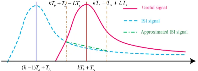
Here, kTb+T∆ accounts for the peak concentration time of the kth symbol, which may be redefined as T∆(k),kTb+T∆. It should be noted that, after the over-sampling process, the discrete signal should be indexed via k andl. For clarity, in the above definition and following analysis, we focus on the convexity
sub-metrics constructed from the2L+1discrete samples that are centered at the peak concentration, which
may be directly indexed by k as in Eq. (19). This is because such convexity sub-metrics c(ki) (i= 1,2,3)
may be of more significance to the estimation of unknown symbols αk. However, for more general cases
where the analyzed samples are not centered at peak concentrations (e.g. kTb+T∆+l0Ts), the constructed
convexity sub-metrics should be indexed by k and l0 jointly, e.g. ck,l0. Since the construction of general convex sub-metrics is the same as Eq. (19), the expressions will be omitted in the following analysis.
Taking the first metric in Eq. (19) for example, when the information bit is αk = 1, this sub-metric
specified by:
ck =c(1)k +c(2)k +c(3)k . (20)
Remark 3: The convexity metric ck will effectively suppress the ISI generated by the previous (k−k0)
symbols.
Due to the heavy tail and the slow decay of concentration from previous symbols, the residual
in-terference ek−k0 at the kth interval, generated from the (k −k0)th previous symbol, may be linearly approximated by Eq. (21), as demonstrated in Fig. 2.
ek−k0(k, l) = αk−k0 ×y[T∆(k−k0) +lTs],
wαk−k0 ×y[T∆(k−k0) +LTs] +bk−k0 ×(L+l) +o{(L+l) 2},
wCk−k0 +bk−k0 ×(L+l), −L6l ≤L. (21) where Ck−k0 = αk−k0 × y[t− T∆(k − k0) +LTs] > 0 is the intercept of an approximated line, and bk−k0'αk−k0 ×
dy(t)
dt |t=(k−k0)Tb+LTs <0 is its negative slope.
Relying on Eq. (21), in the presence of ISI from the (k −k0)-th time, the expectation of the first
sub-metric of time bin [T∆(k)−LTs, T∆(k) +LTs] can be simplified to:
E{c(1)k } '
−1 2
L
X
l=1
αky[T∆(k) +lTs]−
L 2 I X k0=1
Ck−k0 +
3(L−1) 2 bk−k0
−1 2 L X l=1
αky[T∆(k)−lTs]−
L 2 I X k0=1
Ck−k0 + L−1
2 bk−k0
+L×
"
αky(T∆(k)) +
I
X
k0=1
(Ck−k0 +bk−k0L)
#
,
=αk×
(
Ly[T∆(k)]−
PL−1
l=1 [y(T∆(k) +lTs) +y(T∆(k)−lTs)]
2 ) + I X k0=1
(2Lbk−k0 −2L 2
bk−k0).
(22)
Similarly, the expectations of the second and third sub-metrics will be simplified, i.e.,
E{c(2)k }=
αk
2 ×
L−1
X
l=1
{y[T∆(k) +lTs] +y[T∆(k) +LTs−lTs]
E{c(3)k }=
αk
2 ×
L−1
X
l=1
{y[T∆(k) +lTs] +y[T∆(k) +LTs−lTs]
−y[T∆(k) + (l+ 2)×Ts]−y[T∆(k) +LTs+ (l+ 2)×Ts]}.
It is noted from Eq. (22) that the expectation of the first sub-metric c(ki) will be independent of the additive noise. This is because the constructed convex sub-metrics involve only the linear summation or
subtraction operations of the zero-mean noise samples. In Eq. (22), the first term αk×µ1 accounts for the useful signal with µ1 , Ly(T∆(k))− 12 ×PL
−1
l=1[y(T∆(k) +lTs) +y(T∆(k)−lTs)] >0, the second term PI
k0=1(2Lbk−k0 −2L 2b
k−k0) → 0 may be dropped, as the decay slope usually is very small for a large k0, i.e. bk−k0 → 0. So, the convexity metric ck will suppress the ISI from the previous (k−k0)-th time interval. Similar conclusions can be drawn to the other two convexity sub-metrics.
From the simplified expression of c(1)k , an explanation will be further given on how the convexity sub-metrics could suppress ISI. In the case of αk = 1, the convex shape will occur around the peak
concentration, so we have ck significantly larger than zero. Note that, even though the ISI signals from
the previous (k−k0)-th slot may probably exhibit the concave shape, the convexity ofck will almost not
be affected. This is because the diffusion response usually exhibits the long tail, and the ISI signal from
the (k−k0)-th slot would be approximated by a linear function, which of course will not change the
convex shape of useful signals in the k-th slot. To sum up, the convex shape is determined by the useful
signals related with αk, while the second term as in Eq. (21) will not affect the convexity.
Note from Eq. (22) that, the channel response y(t)will appear in the expectation of convex metric c(1)k . This is just to illustrate the composition of c(1)k under different symbols αk. In practice, the calculation
of the three convexity metrics will rely only on the received concentration r(t), as in Eq. (19). By
directly employing the underlying received signal r(t)instead of the channel response y(t), the designed
convexity-based scheme can be regarded as a non-coherent detector.
With the above derivations, the expectation of the local convexity metric becomes:
and the MA length L, i.e.,
µ2 ,
1
2×
L−1
X
l=1
{y[T∆(k) +lTs] +y[T∆(k) +LTs−lTs)]
−y[T∆(k) + (l+ 1)×Ts]−y[T∆(k) +LTs+ (l+ 1)×Ts]},
µ3 ,
1
2×
L−1
X
l=1
{y[T∆(k) +lTs] +y[T∆(k) +LTs−lTs]
−y[T∆(k) + (l+ 2)×Ts]−y[T∆(k) +LTs+ (l+ 2)×Ts]}.
In order to design a decision threshold, we should investigate the expected values of the constructed
convexity metric in the presence of different information bits. Provided that we have the zero-mean
counting noise, then the expectation of ck in the case of αk= 1 is approximated by:
E{ck|αk = 1}=λN L×
(
y[T∆(k)]−y
T∆(k)− L2Ts
4 +
y[T∆(k)]−y
T∆(k) + L2Ts
4 +
yT∆(k)− L2Ts
−y[T∆(k)−LTs]
4 +
yT∆(k) + L2Ts
−y[T∆(k) +LTs]
4
)
,
(24)
where λ is a weighting factor ranged from 0 to 1, and N denotes the total number of sub-metrics. Here,
we have N = 3. When the information bit of the kth duration is αk = 0, then the expected value will
become:
E{ck|αk = 0} →0.
This is due to the fact the convexity metric ck involves two components in Eq. (22), i.e., the linear
combination of zero-mean noises and the other negligible self-interference term that is related with the
decay slope bk−k0 →0.
3) Post-smoothing: A post-smoothing or post-filtering procedure is further suggested to reduce the
noise. In practice, a similar MA process will be used, i.e., c˘(k) = 2L1
0+1 ×
Pk+L0
l=k−L0ck,l, where the averaging length L0 < L will be set to 2∼3.
Finally, a threshold γ will be used to determine whether the current convexity metric is sufficiently
dominant, and then the information bit of each interval will be estimated as in Eq. (25).
ˆ
αk =
(1, c˘
k> γ,
0, c˘k≤γ.
Here, the threshold γ is of importance to the design of the proposed non-coherent detector, as it serves
as a measure of the strength of local convexity.
4) Threshold design: It can be easily seen that, from the definition of convexity metrics in Eqs. (19)–
(20), the threshold γ will be related to three factors:
1) the length of each convexity sub-metric, namely L (recall that each sub-metric is the linear
combi-nation of L terms);
2) the total number of sub-metrics N;
3) the specific convexity of the received concentration.
For the constructed metric, we have the following constraint relationships:
γ < N L
2 ×
y[T∆(k)]−
y[T∆(k) +LTs] +y[T∆(k)−LTs]
2
, (26)
γ > N L
4 ×L1,L2,L3min,L4∈[−L,L],
L1<L2≤L3<L4
{y[T∆(k) +L2Ts] +y[T∆(k) +L3Ts]−y[T∆(k) +L1Ts]−y[T∆(k) +L4Ts]}.
(27)
Here, the upper bound of the threshold γ is determined by the maximum convex value among all
combinations of received samples when constructing convex sub-metrics, as in Eq. (19). Recall the
molecular number will reach the local maximum at the time T∆(k) of the k-th symbol (see Fig. 2), while
one of the molecular number of times T∆(k)±LTs may achieve the minimum value. Thus, the maximum
value is specified by N L2 ×
y[T∆(k)]− 12 × {y[T∆(k) +LTs] +y[T∆(k)−LTs]} . Similarly, the lower
bound of the threshold will be determined by the minimum convex value among all combinations, as in
Eq. (27).
With the equal priors of αk= 1 and αk = 0, the threshold is determined by:
γ , 1
2 ×(E{ck|αk = 1}+E{ck|αk = 0})
' 1
2 ×λN L×
y[T∆(k)]/2−
y[T∆(k) +LTs] +y[T∆(k)−LTs]
4
.
(28)
It is found from Eqs. (24) and (28) that the threshold γ will be viewed as a linearly equal combination
of the median values in four secant lines, which can roughly reflect the convexity shape of the underlying
diffusion channel. Recall that, the convexity metric ck is also a linear combination of multiple median
values, so the designed threshold may produce the promising detection performance, as demonstrated
remains an open problem. For example, the construction of the convex sub-metrics in Eq. (19) and the
combination strategy in Eq. (20) as well as the threshold may be optimised in future work.
Since the accurate channel response y(t) is unavailable for the non-coherent detection scenario, the
threshold γ can be in practice configured approximately via Eq. (29). In this simplest case, we use the
received sample r(k) as the instantaneous estimation of y(k) within a single interval, i.e.,
ˆ
γ = 1
2×λN L×
r(T∆(k))/2−
r(T∆(k) +LTs) +r(T∆(k)−LTs)
4
. (29)
Alternatively, an adaptive threshold γˆ(k) can be suggested to reduce the influence of noise and further
improve the detection performance. For the static channel with unknown response, we will have:
ˆ
γ(k)'(1−β)׈γ(k−1) +β× λN L
2|Ks|
X
m∈Ks
r(T∆(m))
2 −
r(T∆(m) +LTs) +r(T∆(m)−LTs)
4
,
(30)
where β is a forgotten parameter which is ranged in[0.9 0.99]; the initial threshold estimation can be set
to ˆγ(0) = 0; Ks ⊂ {1,2,· · · , k} accounts for a sub-set of the time slots where its convexity metric is
sufficiently large and |Ks| represents the number of elements, i.e.,
Ks=
m
1≤m ≤k, r(T∆(m))/2−
r(T∆(m) +LTs) +r(T∆(m)−LTs)
4 >0.5×σw
. (31)
It is seen that, as k increases, the effects of additive noise will vanish gradually and the adaptive
threshold γˆ(k) will converge to a stable value, i.e. γ(k) =γ(k−1), and then we have
lim
k→∞γˆ(k) = limk→∞
λN L
2 ×
1
|Ks|
X
m∈Ks
r(T∆(k))/2−
r(T∆(k) +LTs) +r(T∆(k)−LTs)
4
= λN L
2 ×
y(T∆(k))/2−
y(T∆(k) +LTs) +y(T∆(k)−LTs)
4
=γ.
(32)
In the designed adaptive threshold, there are three points need to be noteworthy in practice. (1) In
each symbol interval, the threshold γ(k) will be re-calculated, which is then used to detect the signal.
(2) For the static channel with an unknown response, the received signals of multiple intervals have been
utilized to improve the accuracy of the estimated threshold, as in Eq. (30). (3) For the variant channel,
the threshold could also adapt to channel changes based on the received signals. In the case, the sub-set
the channel is temporarily unchanged. The forgotten parameter β will reflect the correlation of varying
channels. Specifically, the higher the channel correlation, the smaller the forgotten parameter is. Consider
the fast varying channel with a low correlation for example, we may have Kc = 1 and β = 0.99, and
consequently, the threshold γ(k) will be estimated only based on the signal of the kth interval.
C. Theoretical Analysis
Since the convex sub-metrics c(ki) (i = 1,2,3) are all based on the linear combination of the noisy observation r(n), thus the constructed convexity metric ck will be Gaussian distributed under the i.i.d
noises. Thus, the likelihood distributions of the convexity metric ck in the case of two information bits
are respectively given by:
p{ck=x|αk = 1}∼N {x;E{ck|αk= 1},V{ck}}, (33)
p{ck=x|αk = 0}∼N {x; 0,V{ck}}. (34)
Here, V{ck} accounts for the variance of the convexity metric ck. It is seen that V{ck} will be related
with the specific construction method of each sub-metric c(ki) (i= 1,2,3), the averaging length 2L+ 1 as well as the noise variance σ2
w. For simplicity, we assume the analysis length L to be an odd integer. For
the i.i.d noise samples, we can further derive the variance of the convexity metric ck which is constructed
from Eqs. (19) and (20), i.e.,
V{ck}=σw2 ×
"
L2+ 1 +
1 2
2
×(2L−4) + 2×
3 2
2#
,
=σw2 ×(L2−0.5L+ 4.5). (35)
Given the threshold in Eq. (28) and the equal priors for “0” and “1”, i.e.,p(αk= 1) =p(αk = 0) = 0.5,
the theoretical error probability of the designed detection method can be calculated via:
PE =p(αk= 1)× γ
Z
0
p{x|αk = 1}dx+p(αk = 0)×
∞
Z
γ
p{x|αk= 0}dx,
= 1
2erfc
s
E2{ck|αk = 1}
8×σ2
w×(L2−0.5L+ 4.5)
!
. (36)
Note from Eq. (36) that the derived BER performance, which is similar to the theoretical result of the
in the case ofαk = 1. For the proposed non-coherent detector, the analytical BER curve will be unavailable
as the term E2{ck|αk = 1} cannot be determined due to the unknown channel response. However, the
theoretical BER curve demonstrates the influence of related parameters (e.g. L and σ2
w), which can be
used to validate the practical detection performance if E{ck|αk = 1} = 2γ can be estimated, e.g. based
on Eq. (30).
D. Complexity Analysis
It is found that the complexity of the new non-coherent scheme is approximatelyonthe order ofO(L2)+
O(L)summation operations, i.e., requiring no multiplication. The first termO(L2)comes from the moving
average operations, while the second term O(L)is attributed to the calculations of convexity metrics and
the threshold. For the previously mentioned coherent MAP scheme, the number of multiplications are
measured by O(2Iϑ), whereϑ accounts for the complexity of evaluating the involved likelihood function.
For a linear MMSE method, the computational complexity is O(I3). Thus, the required multiplications of
coherent detectors (e.g. O(I3)) increases rapidlywith the increasing of I, whilst the required summations
of the new non-coherent scheme increases with O(L2).
IV. NUMERICALSIMULATIONS
In the simulation studies, we focus on the processing of discrete time samples. While the sample
duration Ts may vary with different applications, the proposed non-coherent detection scheme is basically
independent of any specific Ts. Without loss of generality, the maximum concentration of y(t) is located
at tm = 14×Ts. The information interval is set to Tb = 10×Ts, i.e. Tb < tm. In order to simulate
the discrete channel response, the diffusion coefficient is D = 4.75×10⁻⁸m2/s, the distance is d=65nm
and the sampling time is Ts = 1.05×10⁻⁹s. It is easily noted that the received concentrations will be
always positive, as the ISI has usually a long-tail as demonstrated by measurement [12], [13], which will
be dominant to the additive counting noise. Given a high symbol rate, i.e. Tb < tm, severe ISI will occur
at the receiver after the transmitted signal have propagated via the diffusion channel. Each bit error ratio
(BER) curve is derived numerically based on 106 binary symbols. In the analysis, the average length is
set to L= 5 and a long ISI of I = 30×Tb is assumed. The signal to noise ratio (SNR) is defined as:
SNR,10×log10E
PK
k=1r 2
k
Kσ2
w
!
In the first experiment, we will investigate the effect from different configurations of the decision
threshold γ. It is shown by Fig. 3 that, for the suggested threshold in Eq. (30), the weighting factor λ
will have some impact on the detection performance. Taking SNR = 29 dB for example, the best BER
value of 2.25×10⁻³ will be achieved when λ = 0.5, while the worst BER is about 0.35 if λ = 0.01.
Meanwhile, we have noted that, in the high SNR regions (e.g., > 25 dB), the optimal λ is independent
of SNR. Thus, we may conclude that the weighting factor λ may be set to around 0.5 in practice.
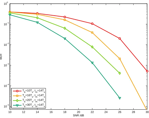
For the non-coherent detection performance, we study the effect of different symbol durations Tb, for a
fixed peak concentration time oftm = 14×Ts. In order to construct the significant and effective convexity
metrics, the symbol duration Tb is expected to be larger than the peak diffusion time, i.e. Tb > tm. It is
easily understood that, the larger the symbol duration Tb, the weaker the ISI from the adjacent durations,
which also results in a more dominant convex shape. The conclusion has been verified by the simulation
results. As demonstrated in Fig. 4, if we increase the symbol duration from Tb = 20Ts w 1.43tm to
Tb = 30Ts w 2.15tm, then a rough detection gain of 2dB will be achieved by the non-coherent scheme.
Although the ISI can be reduced with a sufficiently large Tb, the resulting data rate will be restricted.
Fortunately, we can configure the symbol duration slightly smaller than a peak diffusion time when
pursuing the high data rate, Tb = 0.7× tm. As shown by simulation results, in the serious ISI case
the designed non-coherent detection scheme can also acquire good BER performance. However, this is
achieved at the expense of low energy efficiency (e.g. requiring high SNR). In conclusion, the designed
scheme is relatively robust in the case that the symbol duration is smaller than tm, which is of promise
to promote the data rate of molecular communications.
In Fig. 5, we further plot the theoretical BER curves of our new detection scheme, in which the full
response is assumed to be known. Thus, the expectation on the convexity metric ck can be accurately
evaluated based on Eq. (28). We can see that, for the non-coherent detector, the theoretical BER curve in
Eq. (36) can be interpreted as the low bound, as the threshold γ (or the expectoration on the convexity
metric ck) can only be approximated in practice. From the comparative results in Fig. 5, it is found that
the simulation result agrees with the theoretical BER curves.
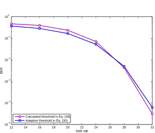
In Fig. 6, the BER performance of the proposed adaptive threshold in Eq. (30) as well as the threshold
calculated from Eq. (28) with a known channel response are plotted together. In the simulation, we
configure the forgotten parameter to β = 0.915. We can see that the adaptive threshold will basically
threshold based on a known channel response may lead to better BER performance. However, in lower
SNRs, the calculated threshold seems to be not accurate. That is mainly because, in the low SNRs (e.g.
SNR 625 dB), the optimal weighting factor λ would be deviated slightly from the configured value 0.5
(see Fig. 3), which may cause the slight degradation on the BER performance. In general, it is observed
that the adaptive threshold can be applied in practice.
A. Comparative Performance
In the second set of experiments, the exact channel response is assumed to be known by the two
previously mentioned coherent detection schemes i.e., the MAP or MMSE schemes, which, of course,
have to be obtained at the expense of sophisticated estimation techniques. In contrast, our proposed scheme
assumes that the channel response is blindto the non-coherent detection process. It is observed that, from
Fig. 7, the coherent MAP scheme can obtain the optimum detection performance, by maximizing the a
posterioriprobability and mitigating the ISI to the minimum. The designed non-coherent detection scheme,
despite the dramatically reduced implementation compared with MAP or MMSE, is slightly inferior to
such coherent schemes. Taking the high SNR regime as an example (e.g., SNR > 22 dB), a detection
SNR gap between our proposed scheme and the MMSE scheme is approximately 2dB.
What is clear from our previous analysis is that, although classical coherent schemes may acquire
the more attractive detection performance, their implementation complexity O(I)3 will become easily
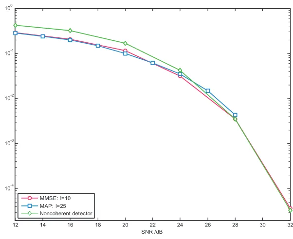
unaffordable as far as a large I is concerned. In order to reduce the computational complexity, as a
compromise, in practice the ISI length I would be truncated to a smaller value. E.g., in some
energy-constrained implementation scenarios, the processing lengthI could be restricted to 10. We observed from
Fig. 8 that, in this case, the MAP detector that changes and becomes comparable to the non-coherent
scheme which, yet, has a much lower complexity than both two coherent schemes. The proposed
non-coherent scheme will achieve a comparable performance with the MMSE method when I = 10.
B. Channel Estimation Error
Although channel parameter estimation is investigated in [31], to the best of our knowledge, the existing
work has not shown how the diffusion channel can be realistically estimated when it is time varying. The
challenge may probably lie in two aspects, i.e., the lack of a chemical pilot signal (due to the limited
chemical bandwidth) and the non-reciprocalnature of a diffusion channel. The reality is that the molecule
differences) and active air flow (movement of bodies). Even when a pilot channel is available, the
non-reciprocal diffusion channel is still difficult to obtain accurately, due to its short coherencetime. Typically,
the channel may change faster than the travel time of molecular signals.
We assume that, for the coherent detectors (i.e. MAP and MMSE), the channel estimation can be
available at a specific time, by resorting to the dedicated chemical pilot. However, the diffusion channel
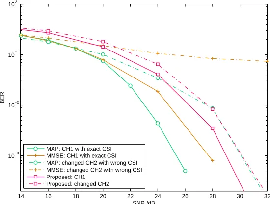
will change randomly after a period of time. For example, the previous channel response CH1 may have
changed to CH2 due to unknown disturbance, as shown in Fig. 9(a). In most cases, coherent detectors will
be unaware of the time-variation of channel response. This is because, in practice, it is very expensive to
employ the bandwidth-demanding pilot to estimate the frequently changed channels for any times. Thus,
they would probablyuse the previously acquired CSI (with errors) until the dedicated chemical pilot can
be attainable again. For the non-coherent method, however we assume it will have no a prioriinformation
on the CSI, and the threshold will be determined based on the received signals as in Eq. (30). Numerical
results in the presence of the varying diffusion channel are demonstrated by Fig. 9(b). As expected, since
the detection performances of the coherent detectors hinges on the channel estimation and, provided an
inaccurate CSI, their BER performances degrade significantly. From the simulation results in Fig. 9(b),
the SNR loss of 5dB may be observed in the MAP scheme. For the MMSE scheme, the BER floor may
even be demonstrated. It is noted that the proposed non-coherent detector relies on the local convexity
of diffusion channel response, which will also update its threshold based on the received signals after
the change in channel response. So, it is essentially independent of the channel estimation and is thereby
robust to unknown CSI. As demonstrated by Fig. 9(b), its BER performance will be affected slightly. This
provides great promise to the realistic application of the non-coherent detector.
V. CONCLUSIONS
A novel non-coherent signal detector is proposed for the emerging field of molecular communications.
The data rate of molecular communications is typically limited by severe ISI, which is difficult to avoid
due to the diffusion process. Whilst up-to-date accurate CSI is difficult to acquire and requires complex
signal processing operations, there exists common features in the diffusion channel that can be exploited
at the receiver side to suppress ISI. By utilizing the local convex features of the channel, the proposed
non-coherent detector can operate in the absence of channel estimations and mitigate ISI from multiple
symbols in high data rate transmissions. In certain channel scenarios, simulation results have shown
coherent detectors. Yet, the signal processing implementation of the proposed non-coherent detector is
simple and involves only a number of summation operations. More importantly, it is found that the
BER performance of the designed scheme, which requires no explicit CSI, is relatively robust to time
varying channels. In general, the proposed low-complexity and non-coherent signal detector will be vital
to the realistic implementation of molecular communications, especially in the application of mobile
molecular communications between nano-robots in the area of nano-medicine, where the low-complexity
implementation is critical.
ACKNOWLEDGMENT
This work of B. Li was supported by Natural Science Foundation of China (NSFC) under Grants
61471061 and the Fundamental Research Funds for the Central Universities under Grant 2014RC0101.
The work of S. Wang was in part supported by the Research Development Fund (RDF-14-01-29) of Xi’an
Jiaotong-Liverpool University.
REFERENCES
[1] I. F. Akyildiz, J. M. Jornet, and M. Pierobon, “Nanonetworks: A new frontier in communications,” Communications of the ACM,
vol. 54, no. 11, pp. 84–89, Nov. 2011.
[2] I. F. Akylidiz, F. Fekri, R. Sivakumar, C. Forest, and B. Hammer, “Monaco: fundamentals of molecular nano-communication networks,”
IEEE Wireless Communications, vol. 19, no. 5, pp. 12–18, May 2012.
[3] T. Nakano, A. Eckford, and T. Haraguchi,Molecular Communications. Cambridge University Press, Oct. 2013.
[4] S. Hiyama, Y. Moritani, T. Suda, R. Egashira, A. Enomoto, M. Moore, and T. Nakano, “Molecular communication,” inProceedings
of the NSTI Nanotechnology Conference and Trade Show, 2005, pp. 391–394.
[5] L. Parcerisa Gin´e and I. F. Akyildiz, “Molecular communication options for long range nanonetworks,”Computer Networks, vol. 53,
no. 16, pp. 2753–2766, Nov. 2009.
[6] T. Nakano, T. Suda, Y. Okaie, M. J. Moore, and A. V. Vasilakos, “Molecular communication among biological nanomachines: A layered
architecture and research issues,”IEEE Transactions on NanoBioscience, vol. 13, no. 3, pp. 169–197, Sep. 2014.
[7] A. W. Eckford, N. Farsad, S. Hiyama, and Y. Moritani, “Microchannel molecular communication with nanoscale carriers: Brownian
motion versus active transport,” in10th IEEE Conference on Nanotechnology (IEEE-NANO), 2010, pp. 854–858.
[8] A. Mafra-Neto and R. T. Card´e, “Fine-scale structure of pheromone plumes modulates upwind orientation of flying moths,”Nature,
vol. 369, no. 6476, pp. 142–144, May 1994.
[9] H. B. Yilmaz, A. C. Heren, T. Tugcu, and C.-B. Chae, “Three-dimensional channel characteristics for molecular communications with
an absorbing receiver,”IEEE Communications Letters, vol. 18, no. 6, pp. 929–932, Jun. 2014.
[10] T. D. Wyatt,Pheromones and animal behaviour: communication by smell and taste. Cambridge University Press, Mar. 2003.
[11] B. Atakan, O. B. Akan, and S. Balasubramaniam, “Body area nanonetworks with molecular communications in nanomedicine,”IEEE
[12] N. Farsad, W. Guo, and A. W. Eckford, “Tabletop molecular communication: Text messages through chemical signals,” PloS one,
vol. 8, no. 12, p. e82935, Dec. 2013.
[13] N. Farsad, N. Kim, A. Eckford, and C. Chae, “Channel and noise models for nonlinear molecular communication systems,” IEEE
Journal on Selected Areas in Communications, vol. 32, no. 12, pp. 2392–2401, Dec. 2014.
[14] W. Guo, S. Wang, A. Eckford, and J. Wu, “Reliable communication envelopes of molecular diffusion channels,”Electronics Letters,
vol. 49, no. 19, pp. 1248–1249, Sep. 2013.
[15] W. Guo, B. Li, S. Wang, and W. Liu, “Molecular communications with longitudinal carrier waves: Baseband to passband modulation,”
IEEE Communication Letters, vol. 19, no. 9, pp. 1512–1515, Jun. 2015.
[16] D. Kilinc and O. B. Akan, “Receiver design for molecular communication,” IEEE Journal on Selected Areas in Communications,
vol. 31, no. 12, pp. 705–714, Dec. 2013.
[17] W.-A. Lin, Y.-C. Lee, P.-C. Yeh, and C.-h. Lee, “Signal detection and ISI cancellation for quantity-based amplitude modulation in
diffusion-based molecular communications,” inIEEE Global Communications Conference (GLOBECOM), 2012, pp. 4362–4367.
[18] A. Noel, K. C. Cheung, and R. Schober, “Optimal receiver design for diffusive molecular communication with flow and additive noise,”
IEEE Transactions on NanoBioscience, vol. 13, no. 3, pp. 350–362, Sep. 2014.
[19] L.-S. Meng, P.-C. Yeh, K.-C. Chen, and I. F. Akyildiz, “On receiver design for diffusion-based molecular communication,” IEEE
Transactions on Signal Processing, vol. 62, no. 22, pp. 6032–6044, Nov. 2014.
[20] B. Tepekule, A. Pusane, M. Kuran, and T. Tugcu, “A novel pre-equalization method for molecular communication via diffusion in
nanonetworks,”IEEE Communications Letters, vol. 19, no. 8, pp. 1311–1314, Aug. 2015.
[21] B. Li, M. Sun, S. Wang, W. Guo, and C. Zhao, “Low-complexity non-coherent signal detection for nano-scale molecular
communica-tions,”IEEE Transactions on NanoBioscience, 2015, doi: 10.1109/TNB.2015.2504542.
[22] M. Pierobon and I. F. Akyildiz, “Information capacity of diffusion-based molecular communication in nanonetworks,” inProceedings
IEEE INFOCOM, 2011, pp. 506–510.
[23] ——, “Diffusion-based noise analysis for molecular communication in nanonetworks,”IEEE Transactions on Signal Processing, vol. 59,
no. 6, pp. 2532–2547, Jun. 2011.
[24] B. Øksendal,Stochastic Differential Equations: An Introduction with Applications. Springer, 2003.
[25] M. Pierobon and I. F. Akyildiz, “A physical end-to-end model for molecular communication in nanonetworks,” IEEE Journal on
Selected Areas in Communications, vol. 28, no. 4, pp. 602–611, May 2010.
[26] H. ShahMohammadian, G. Messier, and S. Magierowski, “Blind synchronization in diffusion-based molecular communication channels,”
IEEE communications letters, vol. 17, no. 11, pp. 2156–2159, Nov. 2013.
[27] S. Kay,Fundamentals of statistical signal processing, volume 1: Estimation theory. Prentice Hall, 1998.
[28] L. S. Meng, P. C. Yeh, K. C. Chen, and I. F. Akyildiz, “On Receiver Design for Diffusion-Based Molecular Communication,”IEEE
Transactions on Signal Processing, vol. 62, no. 22, pp. 6032–6044, Nov. 2014.
[29] M. S. Kuran, H. B. Yilmaz, T. Tugcu, and I. F. Akyildiz, “Modulation techniques for communication via diffusion in nanonetworks,”
inIEEE International Conference on Communications (ICC), 2011, pp. 1–5.
[30] J. G. Prokias,Digital Communication, 3rd ed. McGraw Hill, Oct. 1995.
[31] A. Noel, K. C. Cheung, and R. Schober, “Joint channel parameter estimation via diffusive molecular communication,”IEEE Transactions
noise
[image:25.612.148.463.491.604.2]
Fig. 1. A physical-layer schematic structure of molecular communications.
b
kT T
(k1)TbT
b s
kT TLT kTbTLTs
0 0.1 0.2 0.3 0.4 0.5 0.6 0.7 0.8 0.9 1 10−4
10−3 10−2 10−1 100
λ
BER
[image:26.612.152.458.93.330.2]SNR=31dB SNR=30dB SNR=29dB SNR=28dB SNR=27dB SNR=26dB SNR=25dB
Fig. 3. BER performance of the non-coherent detector with various threshold configurations or different weighting factors.
10 12 14 16 18 20 22 24 26 28 30
10−5 10−4 10−3 10−2 10−1 100
SNR /dB
BER
T
b=10Ts, tm=14Ts
T
b=16Ts, tm=14Ts
T
b=20Ts, tm=14Ts
T
b=30Ts, tm=14Ts
[image:26.612.154.458.443.684.2]10 12 14 16 18 20 22 24 26 28 30 10−5
10−4 10−3 10−2 10−1 100
SNR /dB
BER
Theoretical performance: T b=10Ts Simulated performance: Tb=10Ts
Theoretical performance: Tb=16Ts
[image:27.612.153.458.91.336.2]Simulated performance: Tb=16Ts
Fig. 5. Theoretical BER performance vs simulation results.
12 14 16 18 20 22 24 26 28 30 32
10−5 10−4 10−3 10−2 10−1 100
SNR /dB
BER
Calculated threshold in Eq. (28) Adaptive threshold in Eq. (30)
[image:27.612.152.462.418.685.2]12 14 16 18 20 22 24 26 28 30 32 10-4
10-3 10-2 10-1 100
SNR /dB
B
E
R
[image:28.612.153.461.90.330.2]Sequential MAP (known channel response) Linear MMSE (known channel response) Noncoherent detector (blind)
Fig. 7. BER performance of existing coherent detection schemes (MAP and MMSE) and the proposed non-coherent detection technique.
12 14 16 18 20 22 24 26 28 30 32
10-4 10-3 10-2 10-1 100
SNR /dB
B
E
R
MMSE: I=10 MAP: I=25 Noncoherent detector
[image:28.612.157.458.433.679.2]0 10 20 30 40 50 60 70 80 90 0
0.5 1 1.5 2 2.5
Discrete time index
Channel response
CH1 CH2
(a) Time-varying channel response. CH2 denotes the varied channel response after a period of time.
14 16 18 20 22 24 26 28 30 32
10−3 10−2 10−1 100
SNR /dB
BER
MAP: CH1 with exact CSI MMSE: CH1 with exact CSI MAP: changed CH2 with wrong CSI MMSE: changed CH2 with wrong CSI Proposed: CH1
Proposed: changed CH2
[image:29.612.169.444.395.603.2](b) BER performance of both coherent detection schemes (MAP and MMSE) and the non-coherent scheme with varied channel response