warwick.ac.uk/lib-publications
Original citation:Hladký, Jan, Králʼ, Daniel and Norine, Serguei. (2016) Counting flags in triangle-free digraphs. Combinatorica, 37 (1). pp. 49-76.
Permanent WRAP URL:
http://wrap.warwick.ac.uk/67056
Copyright and reuse:
The Warwick Research Archive Portal (WRAP) makes this work by researchers of the University of Warwick available open access under the following conditions. Copyright © and all moral rights to the version of the paper presented here belong to the individual author(s) and/or other copyright owners. To the extent reasonable and practicable the material made available in WRAP has been checked for eligibility before being made available.
Copies of full items can be used for personal research or study, educational, or not-for profit purposes without prior permission or charge. Provided that the authors, title and full bibliographic details are credited, a hyperlink and/or URL is given for the original metadata page and the content is not changed in any way.
Publisher’s statement:
The final publication is available at Springer via http://dx.doi.org/10.1007/s00493-015-2662-5
A note on versions:
The version presented here may differ from the published version or, version of record, if you wish to cite this item you are advised to consult the publisher’s version. Please see the ‘permanent WRAP url’ above for details on accessing the published version and note that access may require a subscription.
COUNTING FLAGS IN TRIANGLE-FREE DIGRAPHS
JAN HLADK ´Y, DANIEL KR ´AL’, AND SERGEY NORIN
Abstract. Motivated by the Caccetta–H¨aggkvist Conjecture, we prove that every digraph on n vertices with minimum outdegree 0.3465ncontains an oriented triangle. This improves the bound of 0.3532n of Hamburger, Haxell and Kostochka. The main new tool we use in our proof is the theory of flag algebras developed recently by Razborov.
1. Introduction
One of the most intriguing problems of extremal (di)graph theory is the following conjecture of Caccetta and H¨aggkvist [3] dating back to 1978 (we give definitions used throughout the paper in Section 2).
Conjecture 1.1. Everyn-vertex digraph with minimum outdegree at least r has a cycle with length at most ⌈n/r⌉.
For each r and n, there is a whole family of digraphs that are believed to be extremal for the conjecture, see [20]. (And the diversity of these digraphs is probably the reason for the difficulty of the conjecture.) Many results related to the conjecture can be found in a survey by Sullivan [22].
The case when r=n/3 is of particular interest. It asserts that any n-vertex digraph with mini-mum outdegree at least n/3 contains a triangle. Our main result gives a new minimum outdegree bound for this case of the Caccetta–H¨aggkvist Conjecture.
Theorem 1.2. Everyn-vertex digraph with minimum outdegree at least0.3465ncontains a triangle.
Our result improves the previous known minimum-degree bounds established by Caccetta and H¨aggkvist [3] (0.3820n), Bondy [2] (0.3798n), Shen [21] (0.3543n) and Hamburger, Haxell, and Kostochka [9] (0.3532n).
The proof of Theorem 1.2 uses the framework of flag algebras which was developed by Razborov [17]. This framework provides a general formalism which allows to deal with problems in extremal combi-natorics. Razborov used this approach to solve a long-standing open problem on density of triangles in graphs [18], and a special case of the Tur´an’s problem for 3-uniform hypergraphs [19]. After posting the first version of this manuscript, several other applications of flag algebras appeared, see e.g. [1, 5, 6, 8, 10, 11, 13, 16]. In particular, Razborov [20] proved Conjecture 1.1 with r=n/3 for digraphs avoiding three specific digraphs on four vertices. In addition, a software package that can be used to apply flag algebra methods to extremal combinatorics was developed by Vaughan. The package is publicly available at http://www.maths.qmul.ac.uk/∼ev/flagmatic/.
There are two more ingredients that we use in addition to the standard use of flag algebras, which is also referred to as the “semidefinite method” by Razborov. One of them is a variant of inductive arguments which can be found in [17] and the other is a result of Chudnovsky, Seymour and Sullivan [4] on eliminating cycles in triangle-free digraphs. A brute force computer search
was used to combine these ingredients to give the bound. However, the resulting proof is close to being computer-free, only with Maple used to verify several hundred addition and multiplication operations involving five-to-nine digit numbers.
The paper is organized as follows. In Section 2 we present the notation used in the paper and we survey the framework of flag algebras as needed in our proof. The structure of triangle-free digraphs is treated in Section 3. It contains a statement of the key Theorem 3.3 and gives a short proof of Theorem 1.2 based on it. Finally, we give a proof of Theorem 3.3 in Section 4.
2. Notation
We start with introducing a general notation related to directed graphs. A digraph is a directed graph with no loops, no parallel edges, and no counter-parallel edges. A subdigraph of a digraph
D is a digraph that can be obtained from D by deleting some of its vertices and edges. Given a digraphD and a set U ⊆V(D) we write D\U for the subdigraph of D obtained by deleting the vertices of U and D[U] for the subdigraph induced by U, i.e. the subdigraph obtained by deleting all vertices except for those in U. A cycle of length t is a digraph Ct with t vertices v0, . . . , vt−1
and tedges vivi+1 (indices modulo t). A triangle is a cycle of length three. Finally, a digraph is
acyclic if it does not contain any cycle as a subdigraph.
If D is a digraph, we write V(D) and E(D) for the set of vertices and for the set of edges of a digraph D. A vertex v is an outneighbor of u if D contains an edge uv. The outneighborhood Γ+(u) of a vertex u ∈ V(D) is the set of all outneighbors of u, i.e. Γ+(u) = {v ∈ V(D) : uv ∈ E(D)}. Theoutdegree of a vertex u, denoted by deg+(u), is the number of its outneighbors, i.e. deg+(u) = |Γ+(u)|. For a set U ⊆ V(D), the common outneighborhood of U is the set of the
common outneighbors of the vertices contained in U, i.e. Γ+(U) = T
u∈UΓ+(u). A digraph D is outregular if all vertices ofD have the same outdegree. If D is a digraph, we write δ+(D) for the minimum outdegree of a vertex ofD, i.e. δ+(D) = min
u∈V(D)deg+(u).
2.1. Flags. A thorough introduction to flag algebras can be found in [17]. Here, we present those concepts needed in our proof of Theorem 1.2. We follow the notation as used in [17] but we restrict our presentation to the case of triangle-free digraphs. So, we will be dealing (using the language from [17]) with the theory T of triangle-free digraphs, which is a vertex-uniform theory with amalgamation property. The former means that there exists a unique (up to isomorphism) one-vertex digraph and the latter represents the fact that union of two triangle-free digraphs is a triangle-free digraph.
We will introduce an algebra with addition and multiplication on formal linear combinations of unrooted and rooted digraphs, which we will refer to as flags. In the case of rooted digraphs, we want to refer to the subgraph induced by the roots as a type. Formally, a type of order k is a triangle-free k-vertex digraphσ on the vertex set V(σ) = [k]. We will write|σ|for the order of σ, i.e. |σ|=k. A σ-flag is a pair F = (D, θ) where D is a triangle-free digraph and θ: [k]→ V(D) is an isomorphism of σ and D[Im(θ)]. A particular example of a σ-flag is the flag comprised ofσ
and the identity mapping on [k]; slightly abusing the notation, we will use σ for thisσ-flag. Since we think of σ-flags as rooted atσ, we sometimes refer to the vertices of Im(θ) as to the roots.
We now define two different notions of a restriction: a restriction of aσ-flag and a restriction of a type. A restriction of a σ-flag F = (D, θ) to a set U ⊆V(D) such that Im(θ)⊆U is the σ-flag (D[U], θ) which will be denoted by F|U. A restriction of a type σ of order kfor an injective map
η: [k′]→[k] is the typeσ
η with vertex set [k′] and with ij being an edge iff η(i)η(j) is an edge in
σ. In particular, (σ, η) is a ση-flag of order |σ|.
Suppose that σ is a type of order k. We write Fσ for the set of all σ-flags and Fσ
ℓ for those of order ℓ. We will consider two σ-flags F1 = (D1, θ1) and F2 = (D2, θ2) to be isomorphic if there
Figure 1. Example of usage of dashed arrows and grey solid lines.
Figure 2. Frequently used types and flags.
Im(θ1) isθ2◦θ1−1. If twoσ-flagsF1 andF2 are isomorphic, we writeF1 ∼=σ F2. As a slight extension
of this notation, we will useF for the set of all digraphs, Fℓ for the set of all digraphs of order ℓ, and F1 ∼=F2 to denote that F1 and F2 are isomorphic. To ease our way of expressing, we will also
think of F andFℓ as ofFσ andFσ
ℓ for the empty typeσ.
2.2. Frequently used flags. We now introduce notation for the most frequently used flags. The notation is illustrated in Figure 2. For depicting digraphs (also see Figure 1 for illustration), we use solid line arrows to show oriented edges, and dashed lines to depict their absence. When two vertices are not connected by an arrow or a dashed line in a figure, the pair is connected with a grey solid line. This represents that the pair should be expanded into a formal sum of three flags (non-edge and the two orientations of an edge). A dashed arrow in a figure represents a formal sum of two flags with a non-edge and an edge in the opposite direction of the arrow.
The symbol λdenotes the unique type of order one. As explained earlier, we will also useλfor theλ-flag (λ,id). The digraph consisting of a single directed edge is ̺. Theλ-flags obtained from
̺ by labelling the tail and the head are denoted byα and ¯α, respectively. The type consisting of a single directed edge isβ.
Theλ-flag consisting of two vertices, one of them being the root, isγ. Thefork, which is denoted by κ, is the digraph that consists of three vertices a, b, c and two edges aband ac. The vertex ais called the center of κ. When the fork is rooted at its center, it becomes a λ-flag denoted by χ.
2.3. Flag algebras. We shall now enhance Fσ with the structure of an algebra. The motivation for the definitions now presented becomes clear in the next subsection where we introduce the convergence of σ-flags. To give at least a partial motivation for the definitions we now present, let us say that the structure we define on Fσ should behave consistently with the probabilities of seeing theσ-flags involved in a large σ-flag.
IfF′ and F are two digraphs of orders ℓ′ ≤ℓ, respectively, then
p(F′;F) =P
F[U]∼=F′
where U is a random ℓ′-element subset of V(F). Note that we use bold letters to denote random
objects following the notation used e.g. in [17]. The definition can be extended toσ-flags by picking a random subset of non-root vertices. Formally, if F = (D, θ)∈ Fσ
ℓ and F′ ∈ Fℓσ′ are two σ-flags,
ℓ′≤ℓ, we define the quantity p(F′;F) by
p(F′;F) =P
F|Im(θ)∪V∼=σ F′
,
whereVis an (ℓ′− |σ|)-element subset ofV(D)\Im(θ) taken uniformly at random. Note that this
is consistent with viewingF andFℓ asFσ andFℓσ withσ being the empty type. For completeness, we define p(F′;F) to be zero if the order of F′ is larger than the order of F. This allows us to
view the valuesp(F′;F) for a fixedσ-flagF as a vector indexed byFσ: so, we definepF to be the vector from [0,1]Fσ
such thatpF
F′ =p(F′;F).
Lemma 2.1. Let σ be a (possibly empty) type and let ℓ′ ≤ℓ˜≤ℓ, F ∈ Fσ
ℓ and F′ ∈ Fℓσ′. It holds
that
p(F′;F) = X
˜
F∈Fσ
˜
ℓ
p(F′; ˜F)p( ˜F;F).
Informally speaking, Lemma 2.1 says that the probabilities of seeing a σ-flag of orderℓ′ can be
computed from those of seeingσ-flag of order ˜ℓfor some ˜ℓ > ℓ′. This leads as to the definition of an algebraAσ that follows. We consider theKσ of the spaceRFσ of finite formal linear combinations
of σ-flags that is generated by the combinations of the form
F′− X ˜
F∈Fσ
˜
ℓ
p(F′; ˜F) ˜F , (2.1)
for all σ-flag F′ ∈ Fσ
ℓ′ and all pairs ℓ′ and ˜ℓ such that ℓ′ ≤ℓ˜. We then set Aσ =RFσ/Kσ. The
factor-spaceAσ inherits the additive structure fromRFσ. In what follows, we identify the elements of RFσ with their classes in Aσ, i.e. when we speak about the σ-flag F as an element of Aσ, we
mean the classF +Kσ.
We now aim at defining the product operation on Aσ. The motivation again comes from the definition of convergence given in the next subsection. If F1 ∈ Fℓσ1, F2 ∈ F
σ
ℓ2 and F ∈ F
σ ℓ, ℓ ≥
ℓ1+ℓ2− |σ|are threeσ-flags, we define the quantity p(F1, F2;F) to be
p(F1, F2;F) =P
F|Im(θ)∪V1 ∼=σ F1 and F|Im(θ)∪V2 ∼=σ F1
.
where (V1,V2) is a pair of disjoint subsets of V(D)\Im(θ) of cardinalities ℓ1− |σ| and ℓ2− |σ|,
respectively, drawn uniformly at random from the space of all such pairs. This definition allows us to define a bilinear mapping· :Fσ ⊗ Fσ →RFσ as
F1·F2 = X
F∈Fσ ℓ
p(F1, F2;F)F
where F1 ∈ Fℓσ1, F2 ∈ F
σ
ℓ2 and F ∈ F
σ
ℓ, ℓ ≥ ℓ1 +ℓ2 − |σ|. The mapping · can be extended by linearity to RFσ ⊗RFσ. It can be shown [17] that Kσ defines a congruence with respect to this
mapping and the mapping · gives a well-defined multiplication operation in Aσ =RFσ/Kσ. The unit element with respect to the multiplication is the σ-flagσ (recall that we identify the elements
RFσ with their classes in Aσ).
2.4. Convergence. The notions presented in this subsection provide motivation for the definitions we have introduced earlier. Fix a type σ. A sequence of σ-flags {Fn}∞
n=1 converges to a point x ∈ [0,1]Fσ
if the sequence {pFn}∞
n=1 converges to x in the product topology on [0,1]F σ
. The vector x gives rise to a mapping Ψ : Aσ → R defined by Ψ(F) := x
F for F ∈ Fσ and extended linearly to Aσ. It can be shown [17] that if the orders of F
n grow to infinity, then the mapping Ψ is a homomorphism fromAσ to R. We then write lim
n→∞Fn= Ψ.
Let Hom(Aσ,R) be the set of all algebra homomorphisms fromAσ to Rand let Hom+(Aσ,R)⊆ Hom(Aσ,R) be those homomorphisms Ψ such that Ψ(F) ≥ 0 for every F ∈ Fσ. Note that the
homomorphism Ψ defined in the previous paragraph belongs to Hom+(Aσ,R). This correspondence goes both ways as stated in the next theorem (cf. [14, Theorem 2.5], [17, Theorem 3.3]).
Theorem 2.2. Let σ be a type. For every Ψ∈ Hom+(Aσ,R), there exists a sequence of σ-flags {Fn}∞n=1 with growing orders that converges and nlim→∞Fn= Ψ.
On the other hand, if{Fn}∞n=1 is a sequence ofσ-flags with orders growing to infinity, then there
exists a subsequence{Fni}
∞
i=1 of the sequence{Fn}∞n=1 that converges andnlim→∞Fni ∈Hom
+(Aσ,R).
Note that a particular corollary of Theorem 2.2 is that Ψ(F)∈[0,1] for every Ψ∈Hom+(Aσ,R) and every F ∈ Fσ.
We now aim to define a partial order≤σ onAσ to compare “densities” in convergent sequences of σ-flags. If a, b∈ Aσ, then a≤σ biff Ψ(a) ≤Ψ(b) for every Ψ∈Hom+(Aσ,R). Observe that if
a, b∈ Aσ are such that b−a=P
F∈FσcFF with all cF ∈R being nonnegative, thena≤σ b.
2.5. Random homomorphisms and averaging. In the previous subsection, we have associ-ated every convergent sequence (Dn)∞n=1 of triangle-free digraphs with a homomorphism Ψ ∈
Hom+(A,R). We now associate it with a probability distribution Pσ on homomorphisms from
Hom+(Aσ,R) for non-empty typesσ. Fix a typeσ of orderksuch that Ψ(σ)>0. Every mapping
θ: [k]→V(Dn) such thatθis an isomorphism fromσtoDn[Im(θ)] yields aσ-flag, which is (Dn, θ), and it consequently leads to a mapping fromAσ to R, which isp(Dn,θ). By choosing the mappingθ
uniformly at random among all injective mappings from [k] toV(Dn) such thatθis an isomorphism fromσtoDn[Im(θ)], we obtain a probability distribution on mappings fromAσ toR. Note that we obtain one probability distribution on mappings fromAσ toRfor eachn∈N. It can be shown (for the natural notion of convergence) that these probability distributions on mappings fromAσ to R converge to a probability distribution Pσ on Hom+(Aσ,R). The rest of this subsection is devoted to formalizing the connection between the homomorphism Ψ∈Hom+(A,R) and the distributions
Pσ.
Fix a type σ of order k and its restriction σ0 =σ|η of order k′ (recall that η : [k′]→ [k]). The
unlabelling of aσ-flagF = (D, θ) is theσ0-flagF|η = (D, θ◦η). Letθ′ : [k]→V(D) be an injective extension of the map θ◦η : [k′] → V(D) taken uniformly at random among all such injective extensions. The quantity qσ,η(F) is the probability that (D,θ′) andF are isomorphicσ-flags. The averaging operator JKσ,η :Aσ → Aσ0 is the linear extension of the map defined on Fσ as
JFKσ,η=qσ,η(F)F|η . When η is the null mapping, i.e. k′ = 0, we write JK
σ instead of JKσ,η for brevity. In the case of
k′ = 1, we also writeJKσ,m instead ofJKσ,η wherem=η(1).
We further develop the correspondence from the first paragraph of this subsection, which corre-sponds to the arguments given below for η being the null mapping. Recall that a type σ of order
k and its restrictionσ0 =σ|η of order k′ are fixed. For a homomorphism Ψ∈Hom+(Aσ0,R) with
Ψ((σ, η)) > 0, we say that the probability distribution Pσ,η on sets of Hom+(Aσ,R) extends the homomorphism Ψ if
Z
Hom+
(Aσ,R)
Ψ(f)Pσ,η(dΨ) = Ψ(JfKσ,η) Ψ(JσKσ,η)
for all f ∈ Aσ. Theorem 3.5 from [17] asserts that an extension always exists and it is unique.
Theorem 2.3. Let σ be a type of order k and let σ0 =σ|η be its restriction. For every homomor-phism Ψ∈Hom+(Aσ0,R) withΨ((σ, η))>0, there exists a unique probability distribution Pσ,η on
Hom+(Aσ,R) that extendsΨ.
If Ψ ∈Hom+(Aσ0,R) is fixed, then the random homomorphism rooted at σ is a random
homo-morphism given by the unique distributionPσ,η that extends the homomorphism Ψ. The random homomorphism rooted atσ is denoted byΨσ,η. It follows from the definition of the extension that
E[Ψσ,η(f)] = Ψ(JfKσ,η)
Ψ(JσKσ,η) , (2.2)
the first paragraph extend the homomorphism Ψ ∈ Hom+(A,R) associated with the convergent
sequence (Dn)∞n=1 of digraphs.
2.6. Minimum outdegree. The notion of a random homomorphism leads to a natural definition of the minimum outdegree δα(Ψ) of a homomorphism Ψ∈Hom+(A,R). This is defined by
δα(Ψ) = sup{a : P[Ψλ(α)< a] = 0}.
It is not true that if a sequence {Dn}∞
n=1 of digraphs converges to Ψ, then
lim n→∞δ
+(D
n)/|V(Dn)|=δα(Ψ) .
For example, ifDnconsists of a single isolated vertex and a digraph formed by four sets ofnvertices
U1, U2, U3 and U4 with edges going from Ui to Ui+1 (indices modulo four), then the sequence
{Dn}∞
n=1 converges, δ+(Dn) = 0 for every n and δα(Ψ) = 1/4 for the limit homomorphism Ψ. However, the converse is true: if all digraphs Dn have large minimum outdegree, then δα(Ψ) for the limit homomorphism Ψ is also large [17].
Theorem 2.4. Suppose that{Dn}∞
n=1 is a sequence which converges to Ψ. Then
δα(Ψ) ≥lim inf n→∞
δ+(Dn) |V(Dn)|
.
As discussed above, the converse of Theorem 2.4 need not hold in general. However, a weaker statement is true: for every homomorphism Ψ with large minimum outdegree, there exists a se-quence convergent to Ψ with large minimum outdegree. In fact, a sese-quence of digraphs Dn where
Dn=F ∈ Fnwith probability Ψ(F) converges with probability one and it has the desired property with probability one (cf. [14, Section 2.6]).
Theorem 2.5. For every Ψ ∈ Hom+(Aσ,R), there exists a sequence {D
n}∞n=1 of digraphs that
converges to Ψ, and such that
lim n→∞
δ+(D
n) |V(Dn)|
=δα(Ψ).
We now relate the outdegree distribution of a convergent sequence {Dn}∞
n=1 of digraphs and the
associated homomorphism Ψ∈Hom+(A,R). If Dis a digraph andc∈[0,1], then
S(D, c) := |{v∈V(D) : deg
+(v)
≤cn}|
n .
Recall there exists a unique distribution Ψλ on Hom+(Aλ,R) that extends Ψ. A consequence
of [17, Theorem 3.12] is the following.
Lemma 2.6. Let {Dn}∞
n=1 be a convergent sequence of digraphs with limn→∞Dn = Ψ. It holds that
P[Ψλ(α)≤c]≥lim inf
n→∞ S(Dn, c).
The inequality in Lemma 2.6 can be strict: let Dn be a digraph formed by two sets of n and
n+ 1 vertices with all edges going from the smaller set to the larger one. Then S(Dn,1/2) <1/2, butP[Ψλ(α)≤1/2] = 1.
2.7. Cauchy–Schwarz inequality. One of the frequently used tools in extremal combinatorics is the Cauchy–Schwarz Inequality. Recently, Lov´asz and Szegedy [15] made progress on formalizing its importance in the context of extremal graph theory. They have shown that every linear in-equality between subgraph densities that holds asymptotically for all graphs can be approximated (with arbitrary precision) by finitely many applications of the Cauchy–Schwarz Inequality. How-ever, it might not be possible to prove it exactly as shown by Hatami and the third author [12]. The Cauchy–Schwarz Inequality reads in the language of the flag algebras as follows (cf. [17, The-orem 3.14]).
Theorem 2.7. If σ is a type and σ0 =σ|η is one of its restrictions, it holds that
Ψqf2yσ,η≥0
for all f ∈ Aσ and all Ψ∈Hom+(Aσ0,R).
The proof of Theorem 2.7 follows the next lines. Observe that Ψ′(f2) = Ψ′(f)2 ≥ 0 for every Ψ′ ∈Hom+(Aσ,R) and every f ∈ Aσ. If Ψ((σ, η))> 0, then Ψσ,η(f2) ≥0 and so Ψ(qf2y
σ,η) = Ψ(JσKσ,η)E[Ψσ,η(f2)]≥0. If Ψ((σ, η)) = 0, then Ψ(JfK
σ,η) = 0 for everyf ∈Fσ and the statement is trivial.
2.8. Inductive arguments. To formalize inductive arguments in the language of flag algebras, Razborov [17] introduces the notion of an upward operator. We only use two special instances of this operator which we now define.
Let σ be a type of order k and let σ0 = σ|η be one of its restrictions of order k′. For a σ-flag
F = (D, θ), we defineF ↓η to be theσ0-flag obtained fromF by deleting the vertices corresponding
to σ but not toσ0, i.e.,
F ↓η:=F|η \θ([k]\Im(η)).
The operator πσ,η:Aσ0 → Aσ is defined by its action onFσ|η as follows
πσ,η(F) = X
ˆ
F∈Fσ ˆ
F↓η=F ˆ
F ,
forF ∈ Fσ0. The following properties ofπσ,η were established in [17, Theorem 3.18, Corollary 3.19,
Remark 5].
Theorem 2.8. Let σ2 be a type of order k2, let σ1 = σ2|η21 be one of its restrictions of order
k1 ≤k2, and let σ0 =σ1|η10 be one of the restrictions ofσ1 of order k0 ≤k1, i.e. σ0=σ2|η20 where
η20=η21◦η10. Suppose that Ψ∈Hom(Aσ0,R) is a homomorphism such that Ψ((σ2, η20))>0.
a) For everyf ∈ Aσ0 we have
P[Ψσ1, η10
(πσ1,η10(f)) = Ψ(f)] = 1.
b) For everyf ∈ Aσ1 we have
P[Ψσ1, η10
(f) = 0] = 1 ⇒ P[Ψσ2, η20
(πσ2,η21(f)) = 0] = 1.
Note that the assumption Ψ((σ2, η20))>0 in Theorem 2.8 implies that Ψ((σ1, η10))>0.
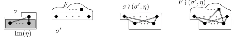
The second operator we define we refer to as the replication operator. Let σ be a type of order
k, let η : [k−1]→ [k] be an injective mapping, and let σ′ be a flag of orderk′. Further, let i
0 be
the unique integer contained in [k]\Im(η). We will define a flagσ′≀(σ, η) of orderk+k′−1. The flag σ′≀(σ, η) is the unique digraph D with vertex-set [k+k′−1] such that ij is an edge of D if
one of the following holds:
Figure 3. The replication operator ≀. From the types σ and σ′ and the σ′-flag F
on the left, we get the typeσ≀(σ′, η) and the σ≀(σ′, η)-flag F≀(σ′, η) on the right.
Two types of lines represent possibly different connection types (non-edges or edges in either direction) inσ, which are then duplicated inσ≀(σ′, η) and F ≀(σ′, η).
• i≥k,j≤k−1 and i0η(j) is an edge ofσ, or
• i≥k,j≥k and (i−k+ 1)(j−k+ 1) is an edge of σ′.
In other words, the vertices 1, . . . , k−1 of σ′≀(σ, η) induce a digraph isomorphic toσ restricted to Im(η), the other k′ vertices of σ′≀(σ, η) are joined to the firstk−1 vertices as the vertexi
0 to the
rest ofσ, and the vertices k, . . . , k+k′−1 induce a digraph isomorphic to σ′. The construction is illustrated in Figure 3.
The definition naturally extends to σ′-flags. IfF′ is a σ′-flag, then the σ′≀(σ, η)-flag F′≀(σ, η) is the unique σ′ ≀(σ, η)-flag F = (D, θ) with |F′|+k−1 vertices such that F ↓η′= F′ where
η′ : [k′]→[k+k′−1] such that η′(x) :=x+k−1, and the remaining edges uu′ of F are defined
as follows:
• ifu∈θ([k−1]) andu′∈θ([k−1]), thenuu′ is an edge iffθ−1(u)θ−1(u′) is an edge of σ,
• ifu∈θ([k−1]), u′ 6∈θ([k−1]), thenuu′ is an edge iffθ−1(u)i0 is an edge of σ, and
• ifu6∈θ([k−1]), u′ ∈θ([k−1]), thenuu′ is an edge iffi
0θ−1(u′) is an edge of σ.
Again, the vertices of θ([k−1]) induce a digraph isomorphic to σ restricted to Im(η), the other vertices of F induce theσ′-flag F′ (after a suitable relabeling), and they are joined to the vertices
inθ([k−1]) as the vertexi0to the rest ofσ. A linear mappingπ≀σ(′σ,η):RF
σ′
→RFσ′≀(σ,η)is defined
by settingπ≀σ(′σ,η)(F′) =F′≀(σ, η) and linearly extending. Note that Kσ ′
does not necessarily lie in the kernel of πσ≀(′σ,η). As before, if σ′ is the empty type, we just writeπ≀(
σ,η).
Fix a type σ of order k and an injective mapping η : [k−1] → [k]. For a homomorphism Ψ∈Hom+(Aσ|η,R), we define Ψ≀(σ,η):A →Ras
Ψ≀(σ,η)(F) :=
Ψ(π≀(σ,η)(F))/(Ψ((σ, η)))|F| if Ψ((σ, η))6= 0, and
0 otherwise. (2.3)
The next theorem, which follows from [17, Theorems 2.6 and 4.1], asserts that the just defined mapping Ψ≀(σ,η) must be a homomorphism of Ato R, in particular, it is well-defined.
Theorem 2.9. Let σ be a type of order k and letη : [k−1]→[k]be an injective map. a) For everyΨ∈Hom+(Aσ|η,R) we have
Ψ≀(σ,η)∈Hom+(A,R).
b) For everyΨ∈Hom+(Aσ|η,R), type σ′ andf ∈RFσ′
ℓ , ℓ∈N, we have
PhΨσ′≀(σ,η), ηπ≀(σ,η)
σ′ (f)
≥0i= 1 ⇒ Ph(Ψ≀(σ,η))σ′(f)≥0i= 1.
To avoid ambiguity, we remark that (Ψ≀(σ,η))σ′ in Theorem 2.9b) stands for Φσ′
where Φ = Ψ≀(σ,η).
Remark 2.10. As an alternative to deriving Theorem 2.9 from [17, Theorems 2.6 and 4.1], which are technical and are stated in the model theoretic language, one can give a direct ad hoc proof of Theorem 2.9.
For the interested reader let us, however, outline the derivation of Theorem 2.9 a) from the results in [17]. The setting we are working in is essentially described in [17, Section 2.3.2]. We apply [17, Theorems 2.6] to the open interpretation (as defined in [17, Definition 3]) (U, I) :T T, where T is the theory of triangle-free digraphs. The formula U represents the diagram of the flag (σ, η)∈ Fσ|η
k andI acts identically. By [17, Theorems 2.6] applied withσ1being the empty type and
σ2 =σ|η, the mapπ(U,I):A → Aσu|η, defined by linearly extending π(U,I)(F) =π≀(σ,η)(F)/(σ, η)|F| forF ∈ F, is an algebra homomorphism. We have Ψ≀(σ,η)=Ψ◦π(U,I), implying Theorem 2.9 a).
3. Structure of triangle-free digraphs
We start with several observations which will later allow us to restrict our attention only to special classes of digraphs.
Observation 3.1. Let D be a triangle-free digraph with δ+(D)≥k. Then there exists a triangle-free digraph D′ on the same vertex set with outdegree of every vertex equal to k.
Indeed, to obtain the digraph D′ it suffices to remove an arbitrary set of deg+(v)−k edges
leavingv for every vertex v.
We next show that a possible counterexample to Conjecture 1.1 would yield counterexamples of arbitrary large order. Suppose that D is an n-vertex triangle-free digraph. Replace each vertex
v∈V(D) by a copyDv of the digraph Dand every directed edgeuv of the original digraphD by a complete directed bipartite graph from Du to Dv. This construction yields a digraphD′ of order
n2. Observe thatδ+(D′) =δ+(D)(n+ 1) and that ifD is triangle-free, then so isD′. We arrive at the following observation by iterating the construction.
Observation 3.2. Suppose that there exists a triangle-free n-vertex digraph D with minimum outdegree at least cn. Then for very m0 there exists a triangle-free digraph D′ of order m > m0
with minimum outdegree at least cm. Moreover, if Dis outregular, then so is D′.
3.1. Caccetta–H¨aggkvist Conjecture in the language of flag algebras. Theorem 3.3 below is the main technical result of the paper. It translates Theorem 1.2 into the flag algebra language.
Theorem 3.3. It holds that
max
Ψ∈Hom+
(A,R)
δα(Ψ)<0.3465.
Theorem 3.3 is proven in the next section. The maximum in Theorem 3.3 is attained by [17, Theorem 3.15]. We now demonstrate that it implies Theorem 1.2.
Proof of Theorem 1.2. Suppose that there exists a triangle-free n-vertex digraphD withδ+(D) =
cn, c ≥ 0.3465. By Observation 3.1 there exists an infinite sequence (Dn)∞n=1 of triangle-free
digraphs with increasing orders such that the digraphDnhas minimum outdegree at leastc|V(Dn)|. By Theorem 2.2, there exists a subsequence (Dni)
∞
i=1 that converges Let Ψ ∈ Hom+(A,R) such
that limi→∞Dni = Ψ. By Theorem 2.4, we haveδα(Ψ)≥0.3465 which violates Theorem 3.3.
Lemma 3.4. Suppose D is a triangle-free digraph with k non-edges. Then there is a vertex v ∈ V(D) withdeg+(v) <√2k.
Lemma 3.4 can be stated in the language of flag algebras as follows.
Lemma 3.5. For every Ψ∈Hom+(A,R) we have for every ǫ0>0 that
PhΨλ(α)<p1−Ψ(̺) +ǫ0 i
>0.
Proof. Let {Dn}∞
n=1 be a sequence of triangle-free digraphs such that limn→∞Dn = Ψ, which exists by Theorem 2.2. The definition of the convergence of a sequence of digraphs yields that for every ǫ >0, there exists a number n0 such that every digraph Dn (n > n0) contains at most
(1−Ψ(̺) +ǫ)|V(Dn)|2/2 non-edges. A repeated application of Lemma 3.4 yields the existence of a set Sn⊆V(Dn), |Sn| ≥ǫ|V(Dn)|, such that deg+(v) ≤(1−ε)−1
p
1−Ψ(̺) +ǫ|V(Dn)| for every
v∈Sn. We conclude using Lemma 2.6 that
PhΨλ(α)≤(1−ǫ)−1p1−Ψ(̺) +ǫi≥ǫ.
The statement of the lemma now follows by choosingǫsufficiently small.
4. Proof of Theorem 3.3
Fix Ψ ∈ Hom+(A,R) with the maximum value of δα(Ψ) in Hom+(A,R) for the rest of the
section (recall that the maximum is attained by [17, Theorem 3.15] as we have already mentioned). Set c0 := δα(Ψ). By considering a sequence of digraphs converging to Ψ and using Theorems 2.2 and 2.5, and Observation 3.1, we can assume without loss of generality that
P[Ψλ(α) =c0] = 1. (4.1)
We proceed by deriving a series of inequalities on the values of Ψ in Subsections 4.2–4.5.
We will concentrate our attention on inequalities which can be expressed in terms of values of Ψ on the elements of F4. To be able to write down these inequalities we will need to enumerate
elements ofF4, and also the elements of F3β and F3λ, which is done in the following subsection.
4.1. Notation. We now fix notation for the elements of F3β,Fλ
3 and F4. The elements of F3β are
denoted byK0, . . . , K7. The vertex set of each of these digraphs is{1,2, a}, where 1 and 2 are the
vertices of β, and the edge set of each of these digraphs is listed in the table below. We will write
K for (K0, . . . , K7)∈ Aβ8.
K0 {12} K1 {12,2a} K2 {12, a2}
K3 {12,1a} K4 {12,1a,2a} K5 {12,1a, a2}
K6 {12, a1} K7 {12, a1, a2}
The symbols L0, . . . L13 denote the elements of F3λ which are considered as digraphs with the
vertex set{1, a, b}, where 1 is corresponds to the vertex of λ. The edge sets are as follows.
L0 {} L1 {ab} L2 {1b} L3 {1b, ab} L4 {1b, ba}
L5 {b1} L6 {b1, ab} L7 {b1, ba} L8 {1a,1b} L9 {1a,1b, ab}
L10 {1a, b1} L11 {1a, b1, ba} L12 {a1, b1}
L13 {a1, b1, ab}
2Ψ1 + 4Ψ10 Ψ3 + Ψ11 + Ψ15 2Ψ2 + Ψ11 + Ψ12 2Ψ4 + Ψ12 + Ψ17 Ψ9 + Ψ13 + Ψ18 Ψ9 + Ψ14 + Ψ19 Ψ3 + Ψ15 + Ψ17 Ψ9 + Ψ16 + Ψ20 Ψ3 + Ψ11 + Ψ15 2Ψ7 + 2Ψ16 2Ψ6 + Ψ14 Ψ17 + Ψ23 + 2Ψ25 Ψ19 + Ψ24 + Ψ27 Ψ18 + Ψ27 Ψ15 + Ψ23 + 4Ψ28 Ψ18 + Ψ29 2Ψ2 + Ψ11 + Ψ12 2Ψ6 + Ψ14 6Ψ5 + 2Ψ13 Ψ12 + 4Ψ21 + Ψ23 Ψ14 + 2Ψ22 Ψ13 + 2Ψ22 + Ψ24 Ψ11 + Ψ23 + 2Ψ25 Ψ13 + Ψ24 + 2Ψ26 2Ψ4 + Ψ12 + Ψ17 Ψ17 + Ψ23 + 2Ψ25 Ψ12 + 4Ψ21 + Ψ23 6Ψ8 + 2Ψ20 Ψ20 + 2Ψ26 + Ψ29 Ψ20 + Ψ29 + 2Ψ30 2Ψ7 + Ψ19 Ψ19 + 2Ψ30
Ψ9 + Ψ13 + Ψ18 Ψ19 + Ψ24 + Ψ27 Ψ14 + 2Ψ22 Ψ20 + 2Ψ26 + Ψ29 2Ψ30 + 2Ψ31 Ψ29 + Ψ31 Ψ16 + Ψ24 Ψ27 + Ψ31 Ψ9 + Ψ14 + Ψ19 Ψ18 + Ψ27 Ψ13 + 2Ψ22 + Ψ24 Ψ20 + Ψ29 + 2Ψ30 Ψ29 + Ψ31 2Ψ26 + 2Ψ31 Ψ16 + Ψ27 Ψ24 + Ψ31 Ψ3 + Ψ15 + Ψ17 Ψ15 + Ψ23 + 4Ψ28 Ψ11 + Ψ23 + 2Ψ25 2Ψ7 + Ψ19 Ψ16 + Ψ24 Ψ16 + Ψ27 2Ψ6 + 2Ψ18 Ψ14 + Ψ27 + Ψ29 Ψ9 + Ψ16 + Ψ20 Ψ18 + Ψ29 Ψ13 + Ψ24 + 2Ψ26 Ψ19 + 2Ψ30 Ψ27 + Ψ31 Ψ24 + Ψ31 Ψ14 + Ψ27 + Ψ29 2Ψ22 + 2Ψ31
[image:12.595.84.514.247.390.2]
Table 1. The matrix AC(Ψ).
Finally, we enumerate the elements of F4, i.e. all isomorphism types of triangle-free digraphs
on the vertex set {a, b, c, d}. The table below gives edge sets of each of these thirty-two digraphs
H0, . . . , H31.
H0 {} H1 {cd} H2 {bd, cd} H3 {bd, dc} H4 {db, dc} H5 {ad, bd, cd} H6 {ad, bd, dc} H7 {ad, db, dc} H8 {da, db, dc} H9 {bc, bd, cd} H10 {ad, bc}
H11 {ad, bc, cd} H12 {ad, bc, bd} H13 {ad, bc, bd, cd} H14 {ad, bc, bd, dc} H15 {ad, bc, db} H16 {ad, bc, db, dc} H17 {da, bc, bd} H18 {da, bc, bd, cd} H19 {da, bc, bd, dc} H20 {da, bc, db, dc} H21 {ac, ad, bc, bd}
H22 {ac, ad, bc, bd, cd} H23 {ac, ad, bc, db} H24 {ac, ad, bc, db, dc} H25 {ac, da, bc, db} H26 {ac, da, bc, db, dc} H27 {ac, ad, cb, db, cd} H28 {ac, da, cb, bd} H29 {ac, da, cb, db, dc} H30 {ca, da, cb, db, cd} H31 {ab, ac, ad, bc, bd, cd}
If Ψ∈Hom+(A,R), we will write Ψi instead of Ψ(Hi) for brevity. So, we can view Ψ = (Ψi)31i
=0 as
an element of R32.
4.2. Cauchy–Schwarz inequalities. Leta∈R8 be a (row) vector. A direct computation gives
that 24Ψ(r(aK⊤)2z
β) = a(AC(Ψ))a
⊤ where A
C(Ψ) is the matrix given in Table 1; the entry
AC(Ψ)ij is Ψ(24JKi·KjKβ) computed by expressingJKi·KjKβ ∈ Aas a sum of elements ofF4.
From Theorem 2.7 we deduce the following.
Corollary 4.1. We have
a(AC(Ψ))a⊤≥0 (4.2)
for everyΨ∈Hom+(A,R) and every a∈R8.
4.3. Outregularity. In this section, we give a simple corollary of (4.1) to frequencies of more general subgraphs.
Lemma 4.2. We have Ψ(Jf·(α−c0)Kλ) = 0 for every f ∈ Aλ.
Proof. Since Ψλ(α −c
0) = 0 with probability one by (4.1) and Ψλ ∈ Hom+(Aλ,R), it follows
that Ψλ(f ·(α−c
0)) = 0 with probability one for every f ∈ Aλ. The statement now follows
from (2.2).
Forb∈R14, we get that
24Ψ(rbL⊤·(α−c0)z
λ) =b(BR−c0AR)Ψ
⊤
AR=
12 6 3 3 3 3 3 3 3 0 0 0 0 0 0 0 0 0 0 0 0 0 0 0 0 0 0 0 0 0 0 0 0 2 2 2 2 0 0 0 0 3 4 2 2 1 1 2 1 2 1 1 1 0 0 0 0 0 0 0 0 0 0 0 0 2 2 2 2 0 0 0 0 3 4 2 2 1 1 2 1 2 1 1 1 0 0 0 0 0 0 0 0 0 0 0 0 0 2 0 0 6 2 0 0 0 0 2 2 4 2 0 0 0 0 0 0 4 4 2 2 2 2 0 0 0 0 0 0 0 0 1 0 0 2 2 0 0 0 1 0 0 1 2 2 1 2 1 0 0 0 2 1 2 0 2 4 1 0 0 0 2 2 2 2 0 0 0 0 3 4 2 2 1 1 2 1 2 1 1 1 0 0 0 0 0 0 0 0 0 0 0 0 0 0 1 0 0 2 2 0 0 0 1 0 0 1 2 2 1 2 1 0 0 0 2 1 2 0 2 4 1 0 0 0 0 0 0 2 0 0 2 6 0 0 0 2 0 0 0 0 2 0 2 4 4 0 2 0 2 2 0 0 2 4 0 0 0 0 0 1 0 0 1 3 0 0 0 1 0 0 0 0 1 0 1 2 2 0 1 0 1 1 0 0 1 2 0 0 0 0 0 0 0 0 0 0 1 0 0 0 1 1 0 1 0 1 1 1 0 2 0 2 0 2 2 0 2 2 4 0 0 0 1 0 0 2 2 0 0 0 1 0 0 1 2 2 1 2 1 0 0 0 2 1 2 0 2 4 1 0 0 0 0 0 0 0 0 0 0 0 1 0 0 0 1 1 0 1 0 1 1 1 0 2 0 2 0 2 2 0 2 2 4 0 0 1 0 0 3 1 0 0 0 0 1 1 2 1 0 0 0 0 0 0 2 2 1 1 1 1 0 0 0 0 0 0 0 0 0 0 0 0 0 0 1 0 0 0 1 1 0 1 0 1 1 1 0 2 0 2 0 2 2 0 2 2 4
BR=
0 1 2 1 0 3 2 1 0 0 0 0 0 0 0 0 0 0 0 0 0 0 0 0 0 0 0 0 0 0 0 0 0 0 0 0 0 0 0 0 0 0 2 2 1 1 1 1 1 0 0 0 0 0 0 0 0 0 0 0 0 0 0 0 0 0 0 0 2 0 0 0 0 2 0 0 1 1 1 0 0 1 1 1 0 0 0 0 0 0 0 0 0 0 0 0 0 0 0 0 0 0 0 0 0 0 0 0 1 1 1 0 0 0 0 0 0 4 4 1 1 0 0 0 0 0 0 0 0 0 0 0 0 0 0 0 0 0 0 0 0 0 0 0 0 1 1 1 0 0 0 1 1 2 0 2 0 0 0 0 0 0 0 1 0 0 0 0 0 1 0 1 0 1 0 1 0 0 1 0 0 0 0 0 0 0 0 0 0 0 0 0 0 0 0 0 0 0 0 0 0 0 0 0 0 0 0 1 1 0 0 0 0 0 0 1 1 0 0 0 4 0 0 0 0 0 0 0 0 0 0 0 0 0 0 0 0 0 0 0 0 1 0 0 1 0 0 1 0 2 2 0 0 1 0 0 0 0 0 0 0 0 0 0 3 0 0 0 0 0 0 0 0 0 0 0 2 0 0 0 0 0 1 0 0 1 1 0 0 0 0 0 0 0 0 0 0 0 0 0 0 0 0 0 0 0 0 0 1 0 0 0 0 0 2 0 0 2 2 3 0 0 0 0 0 0 0 2 0 0 0 0 0 0 0 0 2 0 0 1 0 0 0 0 1 0 0 1 0 0 0 0 0 0 0 0 0 0 0 0 0 0 0 0 0 0 0 0 0 0 0 1 0 0 0 0 1 0 0 1 0 0 2 2 0 0 0 0 0 0 1 0 0 0 0 0 0 0 1 0 0 0 0 0 0 0 1 0 0 0 0 0 0 0 0 0 0 0 0 0 0 0 0 0 0 0 0 0 0 0 0 0 0 0 1 0 0 0 0 0 0 0 0 1 0 1 0 1
Table 2. The matricesAR andBR.
Corollary 4.3. We have b(BR−c0AR)Ψ
⊤
≥0 for everyb∈R14.
Note that the inequality in Corollary 4.3 always holds with an equality.
4.4. Induction. In this section we formalize the inductive argument of Shen [21] in the language of flag algebras and generalize it. Let F = (D, θ) be a σ-flag. We say that F is a σ-source if D
contains no edge from V(D)\Im(θ) to Im(θ). The set of all σ-sources of order k is denoted by Fkσ,→.
Recall thatc0 =δα(Ψ) where Ψ is the homomorphism fixed at the beginning of the section. Let
σ be a type of order k such that the vertex 1 has indegree k−1 in σ, and let F0 = (D, θ) be the σ-flag with |V(D)|= k+ 1 such that every vertex of Im(θ) is connected to the unique vertex in
V(D)\Im(θ) by an outgoing edge. Set
f(σ) :=−c0+X{F : F ∈ Fkσ,+1→, F 6∼=F0}+c0F0 ∈ Aσ . (4.3)
Lemma 4.4. We have Ψ(Jf(σ)Kσ)≥0 for every type σ where the vertex1 has indegree |σ| −1.
Proof. We distinguish two cases. If Ψ((σ,0)) = 0, then Ψ(Jf(σ)Kσ) = 0. Therefore, it suffices to consider the case Ψ((σ,0))>0. We infer from (2.2) that the assertion of the lemma would follow if we proved that
P[Ψσ(f(σ))≥0] = 1.
We now prove this equality.
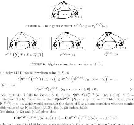
Figure 4. The algebra elementπσ,η1(α) in (4.4) expands into a sum of 2k−1 flags,
each of which is in Fkσ,+1→.
Let k be the order of σ, let F0 = (D, θ) be the σ-flag with |V(D)| = k+ 1 such that every
vertex of Im(θ) is connected to the unique vertex in V(D)\Im(θ) by an outgoing edge, and let
ηi : [1]→[k+ 1] be the mapping such that ηi(1) :=i. If Φ∈Hom+(Aσ,R) is such that Φ(F0) = 0,
then we obtain using triangle-freeness (see Figure 4) that
Φ(πσ,η1(α))
≤ΦX{F : F ∈ Fkσ,+1→, F 6∼=F0} . (4.4) Theorem 2.8 b) and (4.1) (recall that Ψ((σ,0)) > 0) yield that Ψσ(πσ,η1(α)) = c
0 holds with
probability one. This combines with (4.3) and (4.4) to the following: P[Ψσ(f(σ))<0 &Ψσ(F
0) = 0] = 0 .
Therefore, it suffices to show that
P[Ψσ(f(σ))<0 &Ψσ(F0)>0] = 0. (4.5)
We restrict our attention to the case P[Ψσ(F
0) > 0]> 0; otherwise, (4.5) is zero. Let σ′ be the
(unique) type of order k+ 1 such that (σ′, η′)∼=
σ F0 where η′ is the identity mapping from [k] to
itself. Theorem 2.8 b) and (4.1) imply that
P[Ψσ′(πσ′,ηk+1(α
−c0)) = 0] = 1. (4.6)
It follows that
Pσ
Pσ′,η′[(Ψσ)σ′,η′(πσ′,ηk+1(α
−c0)) = 0] = 1
= 1. (4.7)
Indeed, the transition from (4.6) to (4.7) corresponds to samplingσ′ in two steps by sampling first
σ and then extending the sample to σ′.
Thus (4.5) will be established by the following claim.
Claim 4.4.1. For every Φ∈Hom+(Aσ,R) with Φ(F
0)>0 and
P[Φσ′,η′(πσ′,ηk+1(α
−c0)) = 0] = 1 (4.8)
we have
Φ(f(σ))≥0. (4.9)
Proof of Claim 4.4.1. Let ω = α+α+γ be the formal sum of the three elements of Fλ
2. Note
that ω =λif considered as an element of Aλ but we are going to apply the mapping π≀(σ′,η′)
λ and
πλ≀(σ′,η′)(λ) =σ′ 6=π≀λ(σ′,η′)(ω). Also note thatπσ′,η′
(F0) =π≀λ(σ′,η′)(ω) (see Figure 5 for illustration). For every ǫ >0, we have
πσ′,η′(f(σ) +ǫ) =πσ′,η′X{F : F ∈ Fkσ,+1→, F 6∼=F0}+c0F0−c0+ǫ
≥σ′ πσ ′,η
k+1(α
−c0)−π≀(σ
′,η′)
λ (α−(c0+ǫ)ω), (4.10)
since the digraphs considered are triangle-free (see Figure 6). It follows that
PhΦσ′,η′πσ′,η′(f(σ) +ǫ)≥Φσ′,η′πσ′,ηk+1(α−c
0)−π≀(σ
′,η′)
λ (α−(c0+ǫ)ω)
i
Figure 5. The algebra element πσ′,η′
(F0) =π≀(σ
′,η′)
λ (ω).
Figure 6. Algebra elements appearing in (4.10).
The identity (4.11) can be rewritten using (4.8) as
PhΦσ′,η′
πσ′,η′
(f(σ) +ǫ)≥Φσ′,η′
πλ≀(σ′,η′)((c0+ǫ)ω−α) i
= 1. (4.12)
We claim that
P[Φσ′,η′(π≀λ(σ′,η′)((c0+ǫ)ω−α))≥0]>0. (4.13)
Suppose that (4.13) fails for some ǫ > 0. Then P[Φσ′,η′
(π≀λ(σ′,η′)(α −(c0 +ǫ)ω)) > 0] = 1,
and Theorem 2.9 b) would imply that P[(Φ≀(σ′,η′)
)λ(α) ≥ c
0 +ǫ] = 1. This would give that δα(Φ≀(σ
′,η′)
)≥c0+ǫ, which would contradict the choice of Ψ as a homomorphism with the maximum
possible value ofδα(Ψ) in Hom+(A,R). So, (4.13) indeed holds. Combining (4.12) and (4.13) gives that
P[Φσ′,η′πσ′,η′(f(σ) +ǫ)≥0] =P[Φσ′,η′πσ′,η′(f(σ))+ǫ≥0]>0 .
The claimed inequality (4.9) follows by consideringǫց0 and using Theorem 2.8 a), which finishes
the proof of Claim 4.4.1.
The proof of Lemma 4.4 is now also finished.
LetT andV be the types of order 3 withE(T) ={23,21,31}and E(V) ={21,31}, respectively. Note thatT and V are the only types of order 3 satisfying the conditions of Lemma 4.4. We have 24·Ψ(Jf(T)KT) =(1−c0)Ψ9−c0Ψ13−c0Ψ14−c0Ψ16+ (1−c0)Ψ18+ (1−c0)Ψ19+ (1−c0)Ψ20
−2c0Ψ22−2c0Ψ24−2c0Ψ26+ (1−2c0)Ψ27+ (1−2c0)Ψ29
+ (2−2c0)Ψ30−3c0Ψ31,and
(4.14) 12·Ψ(Jf(V)KV) =(1−c0)Ψ2−3c0Ψ5+ (1−c0)Ψ6−c0Ψ11+ (1−c0)Ψ12−2c0Ψ13+ (1−c0)Ψ14
+ (2−2c0)Ψ21−c0Ψ22−c0Ψ23−c0Ψ24−c0Ψ25−c0Ψ26.
(4.15)
The right hand sides of the identities (4.14) and (4.15), which depend on Ψ, are denoted by IndT(Ψ) and IndV(Ψ), respectively. Lemma 4.4 gives the following.
Corollary 4.5. IndT(Ψ)≥0 and IndV(Ψ)≥0.
Figure 7. Graphs involved in Lemma 4.6.
4.5. Density of forks. We now aim at providing a lower bound on Ψ(κ).
Lemma 4.6. Let Φ∈Hom+(Aλ,R) be such that Φ((β,1))>0. If
P[Φβ,1(πβ,2(α)) =c0] = 1, (4.16)
then Φ(γ)≥c0−pΦ(χ).
Proof. By Lemma 3.5 applied to Φ≀(β,1) we have for everyǫ >0 that
P[(Φ≀(β,1))λ(α)<q1
−Φ≀(β,1)(̺) +ǫ]>0. (4.17)
As in Claim 4.4.1, letω=α+α+γ be the formal sum of the three elements ofFλ
2, and let ¯̺∈ F2
be the edgeless digraph on two vertices. Note that ¯̺ = 1−̺ holds in A but π≀(β,1)(¯̺) = χ 6=
π≀(β,1)(1−̺). The inequality (4.17) can be rewritten as
P[(Φ≀(β,1))λ
α−
q
Φ≀(β,1)(¯̺) +ǫ
ω
<0]>0.
By the counterpositive of Theorem 2.9 b) we have
P[Φβ,1
πλ≀(β,1)(α)−
q
Φ≀(β,1)(¯̺)π≀(β,1)
λ (ω)
−ǫ <0]>0 (4.18)
for every ǫ >0. By (2.3) we have Φ≀(β,1)(¯̺) = Φ(χ)/Φ(α)2, as π≀(β,1)(¯̺) =χ. Theorem 2.8 a) and
the identityπλ≀(β,1)(ω) =πβ,1(α) yield thatP[Φβ,1(π≀(β,1)
λ (ω)) = Φ(α)] = 1. We now get from (4.18) that
P[Φβ,1(π≀(β,1)
λ (α))<
p
Φ(χ) +ǫ]>0, (4.19)
for everyǫ >0. It follows from (4.16) and (4.19) that
P[Φβ,1(πβ,2(α)−πλ≀(β,1)(α))> c0− p
Φ(χ)−ǫ]>0. (4.20)
We have πβ,2(α)−π≀(β,1)
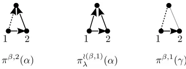
λ (α)≤β πβ,1(γ) (see Figure 7). Thus,
P[Φβ,1(πβ,1(γ))> c0− p
Φ(χ)−ǫ]>0 (4.21)
for everyǫ >0.
We claim that Φ(γ)≥c0− p
Φ(χ). Indeed, suppose for contradiction that Φ(γ) =c0− p
Φ(χ)−ǫ′
for someǫ′>0. By Theorem 2.8 a) we conclude that
PhΦβ,1πβ,1(γ)−c 0+
p
Φ(χ) +ǫ′= 0i= 1,
a contradiction to (4.21). The proof of the claim is now finished.
Proof. The homomorphismΨλsatisfiesΨλ((β,1))>0 and (4.16) with probability one. Therefore, Lemma 4.6 implies that
P
Ψλ(γ) +
q
Ψλ(χ)≥c0
= 1.
Consequently,
E
q
Ψλ(χ)
≥c0−E[Ψλ(γ)] =c0−
1−E[Ψλ(α)]−E[Ψλ(¯α)]= 3c0−1.
The lemma now follows from Jensen’s inequality since Ψ(κ) = 3E[Ψλ(χ)].
We get by expanding κ−3(3c0−1)2 that
4Ψ(κ−3(3c0−1)2) =Ψ4+ Ψ7+ 3Ψ8+ Ψ12+ Ψ17+ Ψ19+ 2Ψ20+ 2Ψ21
+ Ψ23+ Ψ25+ Ψ26+ Ψ29+ 2Ψ30−12(3c0−1)2 31 X
i=0
Ψi .
Let us write Fork(Ψ) for the right hand side of this identity. The next inequality follows directly from Lemma 4.7.
Corollary 4.8. Fork(Ψ)≥0.
4.6. Combining the ingredients. LetR(c) denote the set of vectors r∈R32 such that
(P1) r≥0, (P2) krk1= 1,
(P3) a(AC(r))a⊤≥0 for every a∈R8, (P4) b(BR−cAR)r⊤≥0 for every b∈R14, (P5) IndT(r)≥0 and IndV(r)≥0, and (P6) Fork(r)≥0.
Corollaries 4.1, 4.3, 4.5 and 4.8 imply that Ψ∈R(c0). Therefore, Theorem 3.3 is implied by the
next proposition.
Proposition 4.9. If c≥0.3465, then R(c) is empty.
Proof. Let
a1 = ( −69.83, −27.04, 3.45, −53.59, 1.74, 28.78, −9.28, 59.66 ), a2 = ( −44.57, −25.93, −24.40, −30.16, 2.40, 5.40, 15.67, 37.27 ), a3 = ( 86.95, 58.70, 35.15, 52.46, −18.52, 3.32, −52.56, −57.83 ), a4 = ( −1.29, 0.17, 57.48, −26.29, 10.28, 26.90, −27.33, −9.15 ),
b= (0,0,−17448,−16496,26501,−24163,−8929,−54193,−30136,7267,−24582,−42769,22644,0),
cT = 39648,
cV = 19877 , and
d= 2078.
Further, let
F(c, r) :=
4 X
i=1
ai(AC(r))ai⊤
!
+b(BR−cAR)r⊤+cTIndT(r) +cVIndV(r) +d·Fork(r).
By definition ofR(c), we haveF(c, r)≥0 for every r ∈R(c). Moreover, it can be directly verified (see Maple worksheet, available as an ancillary file on the arXiv) that the function F(c, r) is a
non-increasing function for c∈[1/3,1] if r ≥0 is fixed. On the other hand, we get by computing
F(0.3465, r)
− 38.906394r0 − 25.96859r1 − 4156.34069r2 − 16.447994r3
− 1172.27439r4 − 577.3814r5 − 4.57689r6 − 10.55419r7
− 4042.1489r8 − 10.328894r9 − 13.03079r10 − 1327.03609r11
− 2658.54869r12 − 9.71489r13 − 14574.68439r14 − 7.032994r15
− 6.85949r16 − 11279.04479r17 − 7.458494r18 − 15538.64129r19
− 19.61149r20 − 15.87099r21 − 12.39949r22 − 9949.057894r23
− 9.5492r24 − 12.55709400r25 − 17.24429r26 − 9.535194r27
− 1.24639r28 − 3070.47399r29 − 17.36519r30 − 13.03819r31.
(4.22)
The coefficients in (4.22) are exact. The expression (4.22) is bounded from above byF(0.3465, r)≤
−1.24639krk1<0. Proposition 4.9 follows.
The proof of the proposition concludes the section since Theorem 3.3 is now proven.
5. Concluding remarks
5.1. The algorithm. We now sketch how a computer aided us with a search for the right coeffi-cients used in the estimates. For a fixed value of c, the conditions (P1), (P2) and (P4)–(P6) in the definition ofR(c) give a polytope inR32, which is further denoted byR′(c). The polytopeR′(c) is
defined by 68 linear identities and inequalities. It is not hard to check (using linear programming) whetherR′(c) is empty, while it is less straightforward to verify whetherR′(c) contains a point that satisfies the condition (P3) for every a∈R8. Since a particular pointr ∈R32satisfies (P3) for all
choices aiff AC(r) is positive semidefinite, the search problem for the value cwhen R(c) becomes empty can be expressed as a semidefinite program. However, we have searched for such value c
using an iterative linear programming based algorithm, which required less programming.
5.2. Improving the bound. It is possible to improve the bound we give in Theorem 1.2 slightly at the expense of a more involved proof. As the improvements we were able to produce were not significant and relied on technical and computational tweaks, rather than new ideas. So, we have chosen to present a simpler bound. Still, let us point out some ways to improve the bound we give. 1. Instead of concentrating on the values Ψ takes on elements of F4, one can examine Fk for k = 5,6, . . .. This leads to a significant increase of matrices AC, AR and BR and the involved coefficients in size. R´emi de Joannis de Verclos, Jean-S´ebastien Sereni and Jan Volec pushed the bound in Theorem 1.2 down to 0.3388 in March 2014 by extending the approach presented in this paper. (Their proof uses elementsF6in calculations and it incorporates several additional bounds.)
It seems likely that the bound can be pushed even further.
2. One can attempt to generalize Lemma 4.4. We initially considered a more general class of induction hypotheses but it turned out that adding additional estimates does not lead to further improvements of the bound.
Acknowledgement
The computer search for the coefficients of the vector F(c0, r) was done using QSopt linear
programming solver. We would like to thank its author William Cook for making the tool available and answering our questions concerning its usage. We are also grateful for valuable comments on the manuscript provided by the anonymous referees. Finally, we would like to thank Jean-S´ebastien Sereni for his extremely detailed comments including pointing out typos in some of our formulas.
References
[1] R. Baber and J. Talbot. Hypergraphs do jump.Combin. Probab. Comput., 20(2):161–171, 2011.
[2] J. A. Bondy. Counting subgraphs: a new approach to the Caccetta-H¨aggkvist conjecture. Discrete Math., 165/166:71–80, 1997.
[3] L. Caccetta and R. H¨aggkvist. On minimal digraphs with given girth. InProceedings of the Ninth Southeastern
Conference on Combinatorics, Graph Theory, and Computing (Florida Atlantic Univ., Boca Raton, Fla., 1978),
Congress. Numer., XXI, pages 181–187, Winnipeg, Man., 1978. Utilitas Math.
[4] M. Chudnovsky, P. Seymour, and B. Sullivan. Cycles in dense digraphs.Combinatorica, 28(1):1–18, 2008. [5] J. Cummings, D. Kr´al’, F. Pfender, K. Sperfeld, A. Treglown, and M. Young. Monochromatic triangles in
three-coloured graphs.J. Combin. Theory Ser. B, 103(4):489–503, 2013.
[6] S. Das, H. Huang, J. Ma, H. Naves, and B. Sudakov. A problem of Erd˝os on the minimum number ofk-cliques.
J. Combin. Theory Ser. B, 103(3):344–373, 2013.
[7] M. Dunkum, P. Hamburger, and A. P´or. Destroying cycles in digraphs.Combinatorica, 31(1):55–66, 2011. [8] A. Grzesik. On the maximum number of five-cycles in a triangle-free graph. J. Combin. Theory Ser. B,
102(5):1061–1066, 2012.
[9] P. Hamburger, P. Haxell, and A. Kostochka. On directed triangles in digraphs.Electron. J. Combin., 14(1):Note 19, 9 pp. (electronic), 2007.
[10] H. Hatami, J. Hladk´y, D. Kr´al’, S. Norine, and A. Razborov. Non-three-colorable common graphs exist.Combin.
Probab. Comput., 21(5):734–742, 2012.
[11] H. Hatami, J. Hladk´y, D. Kr´al’, S. Norine, and A. Razborov. On the number of pentagons in triangle-free graphs.
J. Combin. Theory Ser. A, 120(3):722–732, 2013.
[12] H. Hatami and S. Norine. Undecidability of linear inequalities in graph homomorphism densities.J. Amer. Math. Soc., 24(2):547–565, 2011.
[13] D. Kr´al’, C.-H. Liu, J.-S. Sereni, P. Whalen, and Z. B. Yilma. A new bound for the 2/3 conjecture.Combin.
Probab. Comput., 22(3):384–393, 2013.
[14] L. Lov´asz and B. Szegedy. Limits of dense graph sequences.J. Combin. Theory Ser. B, 96(6):933–957, 2006. [15] L. Lov´asz and B. Szegedy. Random graphons and a weak Positivstellensatz for graphs. J. Graph Theory,
70(2):214–225, 2012.
[16] O. Pikhurko and E. R. Vaughan. Minimum number ofk-cliques in graphs with bounded independence number.
Combin. Probab. Comput., 22(6):910–934, 2013.
[17] A. A. Razborov. Flag algebras.J. Symbolic Logic, 72(4):1239–1282, 2007.
[18] A. A. Razborov. On the minimal density of triangles in graphs.Combin. Probab. Comput., 17(4):603–618, 2008. [19] A. A. Razborov. On 3-hypergraphs with forbidden 4-vertex configurations.SIAM J. Discrete Math., 24(3):946–
963, 2010.
[20] A. A. Razborov. On the Caccetta-H¨aggkvist conjecture with forbidden subgraphs.J. Graph Theory, 74(2):236– 248, 2013.
[21] J. Shen. Directed triangles in digraphs.J. Combin. Theory Ser. B, 74(2):405–407, 1998.
[22] B. Sullivan. A summary of results and problems related to the Caccetta–H¨aggkvist conjecture. unpublished, 2006.
Institute of Mathematics of the Academy of Sciences of the Czech Republic, ˇZitn´a 25, Praha. Mathematics Institute is supported by RVO:67985840.
E-mail address: [email protected]
Mathematics Institute and Department of Computer Science, University of Warwick, Coventry CV4 7AL, United Kingdom.
E-mail address: [email protected]
Department of Mathematics & Statistics, McGill University, Burnside Hall, 805 Sherbrooke West, Montreal, QC, H3A 2K6, Canada.