warwick.ac.uk/lib-publications
A Thesis Submitted for the Degree of PhD at the University of Warwick
Permanent WRAP URL:
http://wrap.warwick.ac.uk/80984
Copyright and reuse:
This thesis is made available online and is protected by original copyright.
Please scroll down to view the document itself.
Please refer to the repository record for this item for information to help you to cite it.
Our policy information is available from the repository home page.
AUTHOR:Simon Matthew Bignold DEGREE:PhD
TITLE:Optimisation of the PFC Functional
DATE OF DEPOSIT: . . . .
I agree that this thesis shall be available in accordance with the regulations governing the University of Warwick theses.
I agree that the summary of this thesis may be submitted for publication.
Iagreethat the thesis may be photocopied (single copies for study purposes only). Theses with no restriction on photocopying will also be made available to the British Library for microfilming. The British Library may supply copies to individuals or libraries. subject to a statement from them that the copy is supplied for non-publishing purposes. All copies supplied by the British Library will carry the following statement:
“Attention is drawn to the fact that the copyright of this thesis rests with its author. This copy of the thesis has been supplied on the condition that anyone who consults it is understood to recognise that its copyright rests with its author and that no quotation from the thesis and no information derived from it may be published without the author’s written consent.”
AUTHOR’S SIGNATURE: . . . .
USER’S DECLARATION
1. I undertake not to quote or make use of any information from this thesis without making acknowledgement to the author.
2. I further undertake to allow no-one else to use this thesis while it is in my care.
DATE SIGNATURE ADDRESS
. . . .
. . . .
. . . .
. . . .
M A
O
D
C
S
Optimisation of the PFC Functional
by
Simon Matthew Bignold
Thesis
Submitted for the degree of
Doctor of Philosophy
Mathematics Institute
The University of Warwick
Contents
List of Figures v
Acknowledgements vii
Declarations viii
Abstract ix
Chapter 1 Introduction 1
1.1 Invitation to the Field . . . 2
1.1.1 PFC as a Mesoscopic Model . . . 3
1.1.2 PFC Simulations . . . 4
1.2 Literature Review . . . 5
1.2.1 Modelling . . . 5
1.2.2 Simulations and Applications . . . 6
1.2.3 Numerical Analysis and Scientific Computing . . . 8
1.3 Outline and Summary of Results . . . 10
1.3.1 Outline . . . 10
1.3.2 Summary of Results . . . 11
Chapter 2 Derivation Of the PFC Model 13 2.1 Set-Up . . . 13
2.1.1 The Canonical Ensemble . . . 14
2.1.2 The Helmholtz Free Energy . . . 15
2.2 The One-particle Density . . . 15
2.2.1 Usingδ-functions . . . 15
2.2.2 Integrating theN-particle Density . . . 16
2.2.3 Functional Derivative . . . 17
2.3 The Hohenberg-Kohn Functional . . . 18
2.4 Ideal Gas Contribution . . . 20
2.4.1 Stirling’s Approximation . . . 21
2.5 The Excess Energy Contribution . . . 24
2.5.1 Gradient Expansion . . . 24
2.6 Non-Dimensionalisation and the PFC Model . . . 26
2.7 Discussion . . . 28
2.8 Conclusion . . . 29
Chapter 3 Analysis of the PFC Model 30 3.1 Preliminaries . . . 31
3.2 Minimisation Problem . . . 37
3.3 The Euler-Lagrange Equation . . . 37
3.4 Conclusion . . . 41
Chapter 4 Gradient Flow Analysis 42 4.1 Bochner Spaces . . . 42
4.2 Gradient Flows . . . 44
4.3 SH and PFC Equations . . . 47
4.3.1 Existence . . . 48
4.3.2 Regularity . . . 52
4.3.3 Uniqueness . . . 55
4.4 H2-gradient Flow . . . . 57
4.5 Conclusion . . . 58
Chapter 5 Convergence to Equilibrium 59 5.1 Abstract Convergence Theory . . . 60
5.2 The Lojasiewicsz Gradient Inequality . . . 61
5.3 Compactness . . . 66
5.4 Conclusion . . . 71
Chapter 6 Semi-Discretisation of H2-Flow 72 6.1 Steepest Descent-Type Algorithm . . . 72
6.1.1 Forward Euler Method . . . 72
6.1.2 Adaptive Forward Euler/ Line Search Method . . . 73
6.1.3 Algorithm . . . 74
6.2 Energy Stability and Convergence of Residual . . . 75
6.3 Convergence to Equilibrium . . . 79
6.4 Conclusion . . . 86
Chapter 7 Convex-Concave Splitting 87 7.1 Time Discretisation . . . 87
7.1.1 Backward Euler Method . . . 87
7.1.2 Convex-Concave Splitting . . . 88
7.2 Energy Stability and Convergence of Residual . . . 94
7.3 Convergence to Equilibrium . . . 98
7.4 Conclusion . . . 99
Chapter 8 Implementation 100 8.1 Spatial Discretisations . . . 100
8.2 Review of Time Discretisations . . . 104
8.2.1 Adaptive Convex-Concave Splitting . . . 104
8.2.2 Exponential Convergence . . . 105
8.2.3 Line Search Method . . . 106
8.2.4 Choice of Line Search Algorithm . . . 108
8.2.5 Convergence with Number of Grid Points . . . 110
8.2.6 Domain Convergence . . . 114
8.3 Conclusion . . . 117
Chapter 9 Model Problems 118 9.1 Rotated Crystal . . . 118
9.1.1 Numerics . . . 118
9.1.2 Discussion . . . 119
9.2 Random Initial Conditions . . . 121
9.2.1 Numerics . . . 121
9.2.2 Orientational Ordering . . . 131
9.2.3 Discussion . . . 134
9.3 3D Simulations . . . 134
9.3.1 Vacancy Diffusion . . . 135
9.4 Conclusion . . . 136
Chapter 10 Conclusions and Further Work 138 10.1 Conclusions . . . 138
10.1.1 Novel Algorithms . . . 138
10.1.2 Lojasiewicz Method . . . 139
10.1.3 Equivalence of Discrete Algorithms . . . 139
10.1.4 Divergence at Low Grid Point Numbers . . . 140
10.2 Further Work . . . 140
10.2.1 Coarse-Graining the Solution . . . 141
10.2.2 Evolving Surfaces . . . 143
Appendix A Minimisation of the Hohenberg-Kohn Functional 145 Appendix B Correlation Function 149 B.1 c(1) is constant . . . 149
B.3 ˆc(k) is radial . . . 151
Appendix C Function Space Results 152
C.1 Subspaces ofH2 . . . 152 C.2 Relations between Function Spaces . . . 153
Appendix D Proof of Theorem 5.2.1 158
Appendix E Trust Region Method 163
List of Figures
1.1 PFC Phase Diagram . . . 2
1.2 PFC Solution: Small Test . . . 4
8.1 Unit Cell and Larger Domain . . . 105
8.2 Convergence of Energy . . . 106
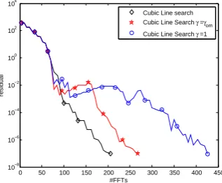
8.3 Residue for the Line Search Method against FFTs : Adaptive Gamma . . . . 109
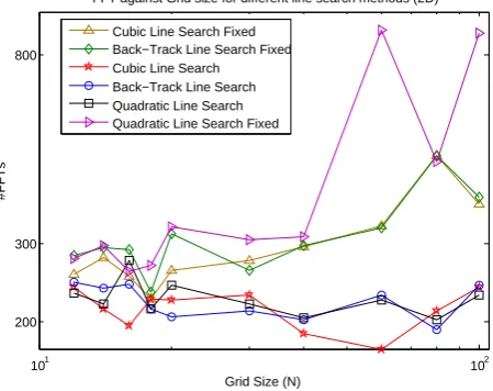
8.4 Convergence of Different Line Search Methods against Grid Size: Fixed Residue110 8.5 Convergence of Different Methods against Grid Size: Fixed Residue . . . 111
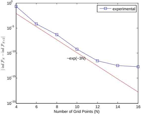
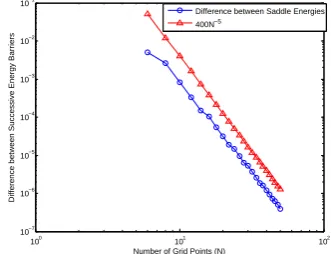
8.6 Saddle Point Energy versus Number of Grid Points . . . 112
8.7 Convergence of Different Methods against Grid Size: Adaptive Residue . . . . 113
8.8 Convergence of Different Methods against Grid Size: Adaptive Residue, Bounded Variations . . . 115
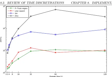
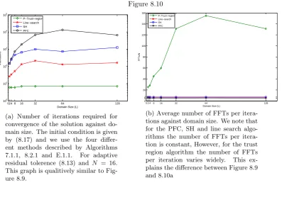
8.9 Convergence of Different Methods against Domain Size . . . 116
8.10 Convergence of Different Methods against Domain Size: Iteration Number . . 117
9.1 Initial Condition: Rotated Crystal . . . 119
9.2 Rotated Crystal after 100000FFTs . . . 120
9.3 Residue Reduction: Rotated Crystal . . . 120
9.4 Residue Reduction: Rotated Crystal LogLog Plot . . . 121
9.5 Random Initial ConditionsL= 64 Domain . . . 122
9.6 Residue Convergence: Random Initial Conditions . . . 122
9.7 Residue Convergence: Random Initial Conditions, LogLog Plot . . . 123
9.8 Residue Against Iteration Number: Random Initial Conditions . . . 124
9.9 Trust Region Metstable Solution: Random Initial Conditions . . . 125
9.10 Fixed Line Search Metastable Solution: Random Initial Conditions . . . 125
9.11 Line Search Metastable Solution: Random Initial Conditions . . . 126
9.12 SH Metastable Solution: Random Initial Conditions . . . 126
9.13 PFC Metastable Solution: Random Initial Conditions . . . 127
9.14 Residue Convergence Metastable State: Random Initial Conditions . . . 127
9.15 Trust Region Solution: Random Initial Conditions . . . 128
9.17 Line Search Solution: Random Initial Conditions . . . 129
9.18 SH Solution: Random Initial Conditions . . . 130
9.19 PFC Solution: Random Initial Conditions . . . 130
9.20 Line Search L=64 Solution: Random Initial Conditions . . . 131
9.21 Line Search L=32 Solution: Random Initial Conditions . . . 132
9.22 Line Search L=128 Solution: Random Initial Conditions . . . 132
9.23 Fixed Line Search L=128 Solution: Random Initial Conditions . . . 133
9.24 Line Search L=256 Solution: Random Initial Conditions . . . 133
9.25 3D Vacancy Initial Conditions . . . 135
9.26 3D Vacancy Final Conditions . . . 136
9.27 Residue Convergence: 3D Vacancy . . . 137
Acknowledgements
The work of this thesis was funded by the MASDOC DTC grant number EP/H023364/1.
First I would like to acknowledge the help of my two supervisors Christoph Ortner
and Charlie Elliott. In particular I would like to thank Christoph, my first supervisor, for
his constant help, support and advice.
I would like to thank Dave Packwood for his help and advice on developing
algo-rithms to address the ‘divergence’ problem of Subsection 8.2.5. I would also like to thank
Antoine Levitt for introducing me to the Lojasiewicz inequality which I have used
exten-sively in Chapters 5-7.
I have really enjoyed my time in Warwick and would like to thank all the members
of the Warwick Mathematics Institute and especially my fellow co-MASDOCs for providing
a stimulating and friendly environment. Particular thanks go to Colin Sparrow for running
a really inspiring and sociable department.
A PhD is a long process and numerous people have contributed their advice and
support, both academically and socially, throughout the last four years. The following list is
therefore probably incomplete and I apologise to anyone I may have inadvertently forgotten.
Firstly I would like to thank the members of my MASDOC year for their support in the three
years that we shared an office. I would also like to thank the residents of B3.04 for letting
me borrow a desk in their office for the last year. Thanks also to the people who shared a
house with me through the first three years of my PhD (Matt, Mike, Kirsty and Andrew).
As well as the above I would also like to thank the many people who provided advice and
entertainment throughout my PhD especially Owen, Steve, Chin, Amal, Abhishek, Alex,
Matt, Yuchen, Felipe, Ben, Huan, Faz, Adam, John, Ollie, Jack, Jamie, Matt, Neil and
Karina.
Declarations
I, Simon Bignold, declare that to the best of my knowledge this work is original and my
own work except when otherwise specified by the references.
The material in this thesis has not to my knowledge been submitted for any other
degree either at this university (the University of Warwick) or any other university. At the
time of submission none of the work within this thesis has appeared or been submitted to
Abstract
In this thesis we develop and analyse gradient-flow type algorithms for minimising the
Phase Field Crystal (PFC) functional. The PFC model was introduced by Elder et al
[EKHG02] as a simple method for crystal simulation over long time-scales. The PFC model
has been used to simulate many physical phenomena including liquid-solid transitions, grain
boundaries, dislocations and stacking faults and is an area of active physics and numerical
analysis research.
We consider three continuous gradient flows for the PFC functional, theL2-,H−1 -andH2-gradient flows. TheH−1-gradient flow, known as the PFC equation, is the typical flow used for the PFC model. The L2-gradient flow is known as the Swift-Hohenberg equation. TheH2-gradient flow appears to be a novel feature of this thesis and will motivate
our development of a line search algorithm.
We analyse two methods of time discretisation for our gradient flows. Firstly, we
develop a steepest descent algorithm based on the H2-gradient flow. We further develop
a convex-concave splitting of the PFC functional, recently proposed by Elsey and Wirth
[EW13], to discretise theL2- andH−1-gradient flows.
We are able to prove energy stability of both our steepest descent algorithm and the
convex-concave splitting scheme of [EW13]. We then use the Lojasiewicz gradient inequality
(first developed in [ Loj62]) to prove that all three schemes converge to equilibrium.
For numerical simulations we undertake spatial discretisation of our schemes using
Fourier spectral methods. We consider a number of implementation issues for our fully
discrete algorithms including a striking issue that occurs when the number of spatial grid
points islow. We then perform several numerical tests which indicate that our new steepest
descent algorithm performs well compared with the schemes of [EW13] and even compared
Chapter 1
Introduction
The Phase Field Crystal (PFC) model was introduced in [EKHG02] as a basic model for crystal simulation. The idea of the PFC model is that we describe the free energy of a particle system by the PFC functional, that is
F[u] = 1
2k∆u+uk
2
L2(Ω)−
δ 2kuk
2
L2(Ω)+
1 4kuk
4
L4(Ω) (1.1)
whereδ >0. We then obtain the equilibrium configuration of the system by minimising the PFC functional under the condition that the mean of the variableu is conserved, that is
− R
udx= ¯u. This constraint is equivalent to mass conservation. [EKHG02] also introduces a basic gradient flow equation to obtain this minimum. This equation, the PFC equation, is written as
ut= ∆[(∆ +I)2u−δu+u3].
The form of the PFC functional can be justified as a combination of a double-well potential, which is minimised by one of two phases, and a functional that is minimised by a periodic density (see [EG04]).
1.1. INVITATION TO THE FIELD CHAPTER 1. INTRODUCTION
By contrast the PFC model has the advantage that it averages out these fast interactions and thus is more suited to addressing large time scales. We discuss this interpretation of the PFC model as a mesoscopic model in Subsection 1.1.1.
In this thesis we analyse and develop various gradient-flow type algorithms to min-imise the PFC functional whilst conserving the average of u. In contrast to some of the literature, e.g. [WWL09] and [EW13], we do not necessarily seek to approximate the trajec-tory of the PFC equation, but instead concentrate on obtaining an algorithm that converges to an equilibrium point.
δ
u
0 −0.05 −0.1 −0.15 −0.2 −0.25 −0.3 −0.35 −0.4 −0.45
0 0.05 0.1 0.15 0.2 0.25 0.3 0.35 0.4 0.45 0.5
[image:14.595.189.462.266.556.2]Fluid Solid Stripes
Figure 1.1: Phase diagram for the PFC model (see [EKHG02, Figure 1a)]). This figure is generated by using the trust region algorithm, Algorithm E.1.1, on the unit cell (see (8.1)) for different values ofδ and ¯u. We start from ¯u= δ = 0, we then succesively increment ¯
uby −0.01 and then increment δ by 0.01. For each new value of δ and ¯uwe obtain the equilibrium solution. The figure is then generated by placing the unit cells next to each other. We note the three phases: liquid, solid and striped.
1.1
Invitation to the Field
1.1. INVITATION TO THE FIELD CHAPTER 1. INTRODUCTION
density. However, a broader and possibly more instructive justification for the PFC model is as an intermediate method between the microscopic method of molecular dynamics (MD, see e.g. [Mel01]) and the macroscopic phase field methods.
1.1.1
PFC as a Mesoscopic Model
The basic hierarchy of models is shown in [WGT+12, Figure 2]. Consider a system of
interacting particles, a MD simulation is obtained by assuming that all particles interact via Newtonian mechanics. The number of coupled equations to be solved increases with the number of particles. This means that MD simulations quickly become impractical.
Density Functional Theory (DFT) is a model of an interacting particle system that is simpler than MD but is still formulated on a microscopic scale. DFT is an equilibrium theory so we can use it to obtain efficient paths from given initial conditions to equilibrium, this is effectively equivalent to coarse-graining the time scale. An introduction to DFT is given in [AM00]. The principle of DFT is that one can describe a particle system by its free energy and that the free energy can be shown to be a functional of the one-particle density (this is the Hohenberg-Kohn Theorem, see Section 2.3). Although in principle the free energy is described by a functional of the one-particle density, in practice this functional is rarely known and is almost always approximated.
The PFC model is obtained by a simple and general method of approximating the free energy functional. We effectively use a curtailed density expansion in both real and Fourier space. More detail on this method is given in Chapter 2. The PFC model is particularly attractive as it has only two parameters, ¯uandδ; c.f. (1.1).
The PFC model creates areas of high density that can be considered as atoms. From PFC simulations (e.g. the vacancy simulation of [EG04, Figure 7]) we can see that the PFC model is coarse-grained in time, that is the fast phonon vibrations are ignored and we act only on a diffusive time scale. Therefore “The PFC method operates on atomic length and diffusive time scales” [WGT+12, page 1].
Two fundamental properties of this model should be highlighted. First, the deriva-tion of the PFC model requires transladeriva-tional and rotaderiva-tional invariance and therefore the minimising density is also translationally invariant along both axes. Translational invari-ance along both axes is a necessary property required for a density that describes a crystalline system. Secondly, by altering the two parameters of the model, the solution obtained tran-sitions between a constant density state (a fluid), and a 2D lattice state (one can see a phase diagram in [EKHG02, Figure 1a)] or Figure 1.1). This means that this model is well suited to solid liquid transition; however, we will not consider this situation in the present work.
1.1. INVITATION TO THE FIELD CHAPTER 1. INTRODUCTION
1.1.2
PFC Simulations
In the previous subsection we remarked that an advantage of the PFC model is that we can view it as a mesoscopic method of particle simulation. A more pragmatic motivation for studying the PFC model is that one can produce simulations that agree with observed phenomena.
We will give references to some PFC simulations that demonstrate physical phe-nomena in Subsection 1.2.2. Of particular interest is the study of [WK07] which shows quantitative agreement between PFC simulations and MD simulations in iron. We note that papers demonstrating such quantitative agreement seem to be rare. However, there is extensive literature on qualitative PFC simulations. These include, but are not lim-ited to, stacking faults (see [BPRS12]), grain boundaries (see [PDA+07]), dislocations (see [EKHG02]), liquid-solid boundaries and colloidal crystal growth (see [GTTP11] for both). We also note that PFC models can be undertaken in both two and three space dimensions without major theoretical changes.
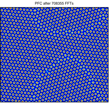
We illustrate a phenomenon that is accessible using the PFC methodology in Fig-ure 1.2. Specifically, we use the PFC equation coming from Algorithm 7.1.1 on a domain sizeL= 32. Using this simulation we see that locally a hexagonal lattice is formed and that grain boundaries are formed at the intersection of these lattice like regions.
[image:16.595.236.415.422.591.2]PFC after 708355 FFTs
Figure 1.2: Solution for the PFC algorithm (Algorithm 7.1.1) after 708355 FFTs starting from random initial conditions given by (9.1) where L = 32. We note the formation of grains.
1.2. LITERATURE REVIEW CHAPTER 1. INTRODUCTION
understanding of the basic PFC model.
1.2
Literature Review
1.2.1
Modelling
We give a brief overview of some of the (many) papers that describe variants of the PFC model and their derivation. We place emphasis on the papers that develop features of the PFC model that we will need in this work. We also outline several review papers that survey the literature surrounding the PFC model. Finally, we mention two theses from the last five years that consider PFC simulations and which provide a good introduction to the topic.
The PFC approach was introduced in the paper [EKHG02]. This paper introduces the PFC functional which describes the energy of the model system. The authors then introduce a basic method for minimising this functional, that is the PFC equation. This paper provides a justification for using the PFC model by showing qualitative agreement between the model and the predictions of Read and Shockley for a grain boundary energy (see [RS50]). Finally, [EKHG02] introduces a binary PFC model which we will not consider in this thesis.
Another important contribution in the development of the PFC model is [EPB+07],
which introduces the idea of deriving the PFC model from DFT. This idea is developed in more detail in Chapter 2.
For the sake of clarity we briefly summarise the modified PFC (MPFC) model. The reason for highlighting this extension to the PFC model is that it seems to be very popular, in particular it is addressed in several of the numerical analysis papers we reference, e.g. [GW14], [GP15] and [WW10]. The MPFC equation was introduced in [SHP06]. The idea of this method is to minimise the PFC functional using a partial differential equation that attempts to incorporate elastic interactions. To obtain the MPFC equation the PFC equation is modified by adding a second-order time derivative, i.e. the MPFC equation is (see [SHP06, Equation (3)])
∂t2u+β∂tu=α2∆δF[u] whereα, β >0.
We now summarise several reviews of the PFC model that outline the key features of the model and collate references to some of the major areas of interest.
An extensive review of work on the PFC model is found in [WGT+12]. This paper reviews the justification for and derivation of the PFC model see [WGT+12, Chapter 1
1.2. LITERATURE REVIEW CHAPTER 1. INTRODUCTION
[EP10] presents the PFC model as a phase field model. This emphasises the link between the PFC methodology and this well developed field. [EP10] also considers the equilibrium properties of the one-mode approximation to the solution of the PFC equation in [EP10, Section 8.4] and the elastic constants of the PFC model in [EP10, Section 8.5].
A recent review of the PFC model is found in [AZ15]. Again, in this paper there is significant focus on the extensions to the original PFC model. However, this paper also outlines work on quantitative applications of PFC-based techniques.
We now outline two theses that focus on the PFC model. Both theses share simi-larities with this work although the specific focus is different in each.
The PhD thesis [Ban11] develops a numerical scheme to solve the PFC equation. The approach used in this thesis is based on a semi-implicit operator splitting (see [Ban11, Subsection 3.1.2]) and also addresses the binary PFC model. This thesis has an extensive literature review in [Ban11, Chapter 2].
The MSc thesis [Lar14] considers the PFC model in both one and two space dimen-sions.
1.2.2
Simulations and Applications
There is extensive literature on qualitative simulations undertaken using the PFC model. References to these can be seen in the reviews detailed above, particularly [WGT+12].
However, we first give a review of work that compares the PFC model and experimental results quantitatively. It should be noted that there appear to be very few papers specifically on quantitative simulations using the original PFC model.
The first paper where a PFC model is compared quantitatively to experimental data is [WK07]. This is also the most well-known quantitative PFC model. The PFC model is compared quantitatively to MD simulations in iron (Fe). The results are shown in [WK07, Table II], we see that there is good agreement in the interfacial free-energy. However, [WK07, Page 8] claims that higher order anisotropies are needed to represent the whole free energy plot and [WK07, Table II] demonstrates that the quantitative agreement with these anisotropies is poor. This issue is also highlighted in [JAEAN09] which suggests that a modification of the PFC model, the eighth-order fitting version of the PFC model (the EOF-PFC), might lead to better quantitative simulations.
A more recent look at quantitative PFC simulations is [AZB14]. Again this paper compares PFC simulations with results from iron (Fe). In this paper the authors compare the PFC results to both MD simulations and experimental results. This paper obtains good quantitative agreement for the surface free energy and the latent heat, see [AZB14, Table V]. This paper notes that there is poor simulation of certain quantities such as the melting expansions (again [AZB14, Table V]) and that since the model is developed for Fe near a melting point it cannot be used for temperatures far from the melting point.
1.2. LITERATURE REVIEW CHAPTER 1. INTRODUCTION
[EKHG02].
A brief overview of several simulations from a variety of PFC models is given in [PDA+07]. [PDA+07, Figure 2] plots grain boundary energy against grain boundary mis-match and shows agreement between the PFC model, the Read-Shockley prediction and experiments in several materials (tin, lead and copper). [PDA+07, Figure 9] shows a 3D simulation with prominent grain boundaries. Grain boundaries are also simulated using a coarse-grained version of the PFC model in [PDA+07, Figure 8]. Finally, this overview
discusses the MPFC equation and the binary PFC model. The MPFC equation is used to simulate dislocation glide in [PDA+07, Figure 6] and the binary PFC model is used for a
variety of simulations, see e.g. [PDA+07, Figure 10].
We now outline several papers that consider PFC simulations of specific phenomena. The first paper we mention considers a situation which is similar to the large simulation we undertake in Section 9.1.
The paper [WV12] simulates grain growth in 2 dimensions using the PFC model in several different situations. [WV12, Section 3] considers a grain embedded within a larger grain where the first grain is misorientated with respect to the larger grain. The evolution of the grain is shown in [WV12, Figure 6]. These simulations are broadly similar to the situation we consider in Section 9.1; however, in our simulations the misorientated grain is much smaller relative to the background grain. This paper also considers a 3-grain simulation in [WV12, Section 4]. 3-grain simulations similar to those of [WV12, Section 4] could be undertaken using the methods described in this thesis; however, for the sake of brevity we do not pursue this option.
We briefly mention some papers that simulate interesting physical phenomena using the PFC model. Although we do not specifically address these phenomena within this thesis, these papers give a brief indication of the scope of the PFC model.
[BPRS12] uses the PFC model to simulate stacking faults. Illustrations of the quali-tative results obtained by this paper are seen in [BPRS12, Figures 1 and 6]. This paper also compares the results obtained for several modifications of the PFC model (see [BPRS12, pages 5-7]).
The letter [HE08] shows that one can simulate the formation of epitaxial islands using the PFC model with an additional cubic term. 2D and 3D simulations of these islands are shown in [HE08, Figure 1]. This paper also uses a coarse-grained model to consider this island formation.
1.2. LITERATURE REVIEW CHAPTER 1. INTRODUCTION
shows heterogeneous nucleation from a square lattice using the same model. This adaptation of the PFC model is also used to simulate colloid patterning and the creation of particle chains, the results of these simulations are compared to experimental results in [GTTP11, Figures 14] and [GTTP11, Figure 16] respectively.
1.2.3
Numerical Analysis and Scientific Computing
In this section we survey some of the papers that undertake numerical analysis of algorithms based on the PFC model. In general these papers focus on discretisations of the PFC equation.
We first highlight two papers that use the Lojasiewicz inequality to prove conver-gence of the MPFC equation. If ϕ is an equilibrium point, the Lojasiewicz inequality is satisfied if there exist constantsc≥0,σ >0 andθ∈ 0,1
2
such that for allη∈u¯+H2
#(Ω)
(see Definition C.1.2 for the definition ofH2
#(Ω)) withkη−ϕkH2(Ω)≤σ
kδF[η]kH−2(Ω)≥c|F[η]− F[ϕ]|1−θ.
We will use the Lojasiewicz inequality extensively in Chapters 5-7. The paper [GW14] uses the Lojasiewicz inequality to prove that the solution of the MPFC equation converges to an equilibrium point of the PFC functional. We use similar methods to those used in this paper in Chapter 5 and use discrete analogues of these methods in Chapters 6 and 7.
The paper [GP15] uses the Lojasiewicz inequality to prove that the solution of a discretisation of the MPFC converges to an equilibrium solution. Although we do not specif-ically consider the MPFC equation we use the Lojasiewicz inequality to prove convergence of our schemes (which include a discretisation of the PFC equation) in Chapters 6 and 7.
We now survey several papers on the discretisation of the PFC equation. We con-clude with the two papers ([WWL09] and [EW13]) that will be of most use for our thesis.
The recent paper [LSL15] introduces an operator splitting method for simulating the PFC equation. The authors introduce first and second order splittings to treat the non-linear term in [LSL15, Equations (10)] and [LSL15, Equation (18)] respectively. Basic numerical tests are undertaken using this method in [LSL15, Section 3]. The approach used by this paper is to split the scheme into linear and nonlinear subequations (see [LSL15, Section 2]). The authors claim that the linear subequation has a closed form in Fourier space. The operator splitting approach of this paper is compared favourably to the first and second order energy stable methods of [HWWL09] in [LSL15, Section 3] (the first order energy stable scheme is based on the method introduced in [WWL09]).
1.2. LITERATURE REVIEW CHAPTER 1. INTRODUCTION
time-step method where the time-step is updated using [ZMQ13, Equation (3.1)]. Finally basic numerical tests are undertaken in [ZMQ13, Section 4].
Another semi-implicit approach to the PFC equation and the associated Swift-Hohenberg (SH) equation is given in [CW08]. The scheme is outlined in [CW08, Equa-tions (4) and (5)]. [CW08, Section 2.2] shows the unconditional stability of the scheme and demonstrates that the Crank-Nicholson approach for the PFC equation is unstable. This paper (see [CW08, Section 2.3]) also considers updates taken in Fourier space, which we also use for our spatial discretisation in Chapter 8.
In [WWL09] the authors develop a time discretisation of the PFC equation using a convex-concave splitting. In [WWL09, Theorem 1.1] it is proved that such a scheme is energy stable. [WWL09] also introduces a space discretisation in Section 2. Finally, in [WWL09, Theorem 3.11] the authors prove an error estimate that shows that the approximation converges to a solution of the PFC equation when the time-step and grid spacing go to zero. We analyse a different convex-concave splitting in Chapter 7.
A finite element method for the scheme of [WWL09] is developed in [HWWL09]. In this paper they also develop a second order scheme for the PFC equation, [HWWL09, Equations (8)-(10)]. A multigrid numerical method for this second order scheme is developed in [HWWL09, Section 5.2]. This scheme is used to simulate heterogeneous nucleation in [HWWL09, Figures 7(a)-(c)].
The most significant reference for our thesis is [EW13]. This paper introduces a new convex-concave splitting to discretise the PFC equation and the SH equation. The existence of a similar scheme is proposed at the end of [HWWL09, Section 2]. The energy splitting used in this paper is
F[u] =FC,Cstab[u]− FE,Cstab[u],
where, forCstab>0,
FC,Cstab[u] =
1
2k∆u+uk
2
L2(Ω)−
δ 2kuk
2
L2(Ω)+
Cstab
2 kuk
2
L2(Ω),
FE,Cstab[u] =
Cstab
2 kuk
2
L2(Ω)−
1 4kuk
4
L4(Ω).
We note that this splitting is only locally convex-concave. In particular FE,Cstab is only
1.3. OUTLINE AND SUMMARY OF RESULTS CHAPTER 1. INTRODUCTION
1.3
Outline and Summary of Results
The aim of this thesis is to develop and analyse various gradient-flow type algorithms to minimise the PFC functional whilst conserving the mass. In particular we focus on obtaining an efficient time discrete algorithm that converges to an equilibrium point of the PFC functional.
1.3.1
Outline
We begin with a basic introduction to the PFC model. In Chapter 2 we outline the method for deriving the PFC model from DFT. The link between DFT and the PFC model was first shown in [EPB+07] and can be used to justify the wide range of potential applications for
the PFC model.
In Chapter 3 we introduce the basic machinery needed to formulate our PFC prob-lem. We introduce the domain Ω and the spaceHu¯2(Ω) from which we will choose our
solu-tion. We also formulate the PFC functional (3.1) and its first and second variations (Lemma 3.1.4). Finally, we show that critical points of the PFC functional satisfy the Euler-Lagrange equations (Lemma 3.3.1) and that the solution to the Euler-Lagrange equations is smooth (Lemma 3.3.3).
In Chapter 4 we introduce a method of reaching critical points of the PFC functional. Specifically, we use the technique of gradient flow (4.1). We introduce three gradient flows namely theH−1-,L2- andH2-gradient flows (Definitions 4.2.1, 4.2.2 and 4.2.4), that is
hut, viL2(Ω)=−δF[u, v] ∀v∈H#2(Ω)
hut, viH−1(Ω)=−δF[u, v] ∀v∈H#2(Ω)
and
h[(∆ +I)2+γI]ut, viL2(Ω)=−δF[u, v] ∀v∈H#2(Ω)
whereγ >0. We then prove the existence of a solution to all three of these gradient flows (Lemmas 4.3.2 and 4.4.1) as well as uniqueness (Lemma 4.3.4) and regularity results (Lemma 4.3.3). TheH2-gradient flow is compared with and motivated by Newton’s method.
After introducing the gradient flow methodology in Chapter 4 we then prove that the solutions of these gradient flows converge to equilibria. In a similar way to [GW14] we use a Lojasiewicz inequality to prove the convergence results and an estimate on their associated convergence rates. We first prove that the Lojasiewicz inequality holds for the PFC functional in the correct space, i.e. H#2(Ω) (Theorem 5.0.1). We then use this result and a theorem of [HJ15] to prove convergence of the solution (Theorem 5.0.2).
1.3. OUTLINE AND SUMMARY OF RESULTS CHAPTER 1. INTRODUCTION
introduce a variable metric approach ((6.3)), that is
[(∆ +I) +γnI]
u
n+1−un
τn
, v
=−δF[un, v] ∀v∈H#2(Ω)
where
γn= max
γmin,3u2n−δ
.
In our simulations of Chapter 9 we show that the variable metric scheme reaches equilibrium faster than the fixed metric scheme. Based on the variable metric approach we formulate an algorithm to reach equilibrium (Algorithm 6.1.1) and show that such an algorithm is energy stable (Proposition 6.2.3). Finally, we use the Lojasiewicz inequality to prove a general theorem that guarantees convergence of our scheme and the associated convergence rates (Lemma 6.3.2).
Chapter 7 extends the results of [EW13]. We first justify and formulate the convex-concave splitting schemes and then show that they are qualitatively similar to our H2
-gradient flow. Using similar techniques to Chapter 6 we can now prove energy stability of the schemes of [EW13] (Lemma 7.2.1) and convergence to equilibrium (Theorem 7.1.3).
In order to demonstrate the validity of our method we numerically test our algo-rithms. To do this we first introduce space discretisation via spectral methods in Chapter 8. We review several methods of choosing a time-step and pick the most efficient ones (Section 8.2). We then perform some basic numerical tests. We first test the effect of the number of spatial grid points on our methods and discuss an issue that arises when the number of spatial grid points is low (Subsection 8.2.5). Finally, we show the effect of the domain size on the convergence time of our algorithms (Subsection 8.2.6).
In Chapter 9 we undertake some larger simulations. We wish to show the potential applications of our method especially on problems that might be interesting to practitioners. In particular, we review simulations based on a lattice with a rotated crystal (Section 9.1) and also based on a random environment (Section 9.2). The rotated crystal environment has already been a focus of some PFC research in [Lar14].
Chapter 10 reviews the results of our thesis and outlines areas of future research.
1.3.2
Summary of Results
Having given a brief overview, we now highlight the novel features of this thesis. First we note that the vast majority of the PFC literature has been developed by the physics community. Therefore, although not unique in its numerical analysis focus, this thesis may provide a useful introduction to researchers more interested in a mathematical approach to the model.
The main novel aspect of this thesis is the introduction of a newH2-gradient flow (Definition 4.2.4). We also introduce a variable metric version of the discrete form of this gradient flow in Subsection 6.1.2.
1.3. OUTLINE AND SUMMARY OF RESULTS CHAPTER 1. INTRODUCTION
techniques. The existence theory for the other two gradient flows is also new although it is also based on well known techniques and similar existence results have been derived before for the PFC equation in different ways, e.g. in [WWL09]. We also prove that the solutions to the SH and PFC equations are continuously differentiable in H2(Ω) given appropriate
initial conditions (i.e. Lemma 4.3.3).
The Lojasiewicz inequality technique of Chapter 5 has been used for the MPFC equation, which is very similar to the PFC equation, in [GW14]. However the application of this method to theH2- and L2-gradient flows seems to be novel.
Since the H2-gradient flow is a new feature of this thesis, Chapter 6, which
fo-cuses on developing an algorithm based on this method, is largely new. We note that the Lojasiewicz inequality has previously been applied to a discrete algorithm for minimising the PFC functional in [GP15]. A particularly interesting aspect of this chapter is the general convergence lemma, Lemma 6.3.2.
Although Chapter 7 focuses on a method developed in [EW13], we derive a new energy stability theorem for this scheme. We also use the Lojasiewicz inequality to prove convergence to equilibrium of this scheme, this convergence result appears to be new. Finally we develop a qualitative link between the scheme of [EW13] and ourH2-gradient flow.
Chapter 2
Derivation Of the PFC Model
To provide a justification for the study of the phase-field crystal (PFC) model, we derive it via a series of approximations from density functional theory (DFT), which is a well-established method in statistical mechanics. The derivation that we give in this chapter will be purely formal.
We start from the statistical mechanics set-up of the canonical ensemble. That is, we have a fixed number of particles with the N-particle density given by ˆρN(XN) = exp[−βHN(XN, U1)](N!ZN(U1,Ω))−1. We choose to focus on a static system with a
pair-wise interaction potential and an external potential that acts equally on all particles. It is then possible to derive the equilibrium one-particle density ρN(x) in three different ways. We also introduce the free energy,FN[U1,Ω] =−β−1ln [ZN(U1,Ω)], as an
important quantity that describes the system. The density is the quantity we will focus on deriving as it will allow us to find the free energy.
We introduce the Hohenberg-Kohn functional and show the free energy can be obtained from the minimisation of the Hohenberg-Kohn functional over all possible
one-particle densities,FN[U1,Ω] = min ˜
ρ
FHK[ ˜ρ] +
Z
Ω
U1(x) ˜ρ(x)dx
. It is also shown that the
minimising density corresponds to the equilibrium density. The Hohenberg-Kohn func-tional is split into an ideal gas part and the excess energy contribution FHK[ρN(x)] =
FHK,id[ρN(x)] +FHK,exc[ρN(x)].
We can then formulate the PFC model by using a sequence of formal approximation steps. The excess energy and ideal gas contribution are both approximated individually and then re-combined to give the PFC functional as an approximation of the Hohenberg-Kohn functional.
2.1
Set-Up
2.1. SET-UP CHAPTER 2. DERIVING THE PFC MODEL
works on the PFC model conserve particle density through their choice of evolution equation (principally using theH−1-gradient flow), see for example [WGT+12] and [EW13].
In general we consider a system of N ∈ N particles where d is the dimension of the system and positions are confined to a finite domain Ω⊂Rd. The Hamiltonian of the system is given by
HN(XN, U1) =
N X
i=1
U1(xi) + X
1≤i<j≤N
U2(|xi−xj|)
where XN = (x1, . . . , xN)∈ΩN, U1 : Rd →R is the external potential and U2 :Rd →R is the interaction potential between particles. For simplicity, we considerU2 as a pair-wise
potential which depends only on the distance between two particles, hence it is rotationally and translationally invariant. We consider a static system; this means the Hamiltonian does not depend on momentum. If we also take particle momentum into account we have no additional difficulties. In fact we would only change the free energy computed below by an additive constant multiplied byN.
2.1.1
The Canonical Ensemble
To describe the statistical mechanics approach to DFT we introduce the canonical Gibbs measure. We define the Canonical Gibbs Ensemble following [Ada06, p.20], where we also introduce aN! factor to account for indistinguishability of particles (this is to resolve the Gibbs paradox, see [Ada06, Section 4.1]).
Definition 2.1.1 (Canonical Gibbs Ensemble). Equip ΩN with the Borel σ-algebra BΩ. Then the probability measureγΩβ∈ P(ΩN,B
Ω)with density
ˆ
ρN(XN) = ˆρN(XN;U1,Ω)
=exp [−βHN(XN, U1)] N!ZN(U1,Ω)
(2.1)
is called the canonical ensemble.
The normalisation constantZN(U1,Ω) is called the partition function, and can
there-fore be written as
ZN(U1,Ω) =
1 N!
Z
ΩN
exp [−βHN(XN, U1)] dXN (2.2) where the constant
β= 1 kBT
,
is the inverse temperature, scaled by Boltzmann’s constantkB.1
1(2.1) can be thought of as a probability measure weighting the various possible micro-states of the
2.2. THE ONE-PARTICLE DENSITY CHAPTER 2. DERIVING THE PFC MODEL
2.1.2
The Helmholtz Free Energy
A quantity of great interest to us is the Helmholtz free energy hereafter referred to as the free energy. The free energy is an important quantity as it can be used to find fundamental quantities of the system including pressure and entropy see [Ada06, page 24]. Following [Ada06, page 23] we know the free energy is given by
FN[U1,Ω] =−β−1ln [ZN(U1,Ω)].
Therefore, using the partition function (2.2), we can write the free energy as
FN[U1,Ω] =−β−1ln
1 N! Z ΩN exp
−β
N X
i=1
U1(xi) + X
1≤i<j≤N
U2(|xi−xj|)
dXN
=β−1lnN!
−β−1ln
Z ΩN exp
−β
N X
i=1
U1(xi) + X
1≤i<j≤N
U2(|xi−xj|)
dXN
.
(2.3)
2.2
The One-particle Density
A fundamental object in DFT is the one-particle density. We present three equivalent ways of defining it. In this section we only consider the equilibrium density. In a later section, Section 2.3, we will introduce notation that allows this to be generalised.
2.2.1
Using
δ
-functions
The canonical definition of the one-particle density (see e.g. [WGT+12, Equation (2)]) is
as the average ofN δ-functions centered at the particle positions, taken with respect to the canonical Gibbs measure (2.1):
ρN(x) =ρN(x;U1,Ω)
= Z ΩN N X i=1
δ(x−xi) ˆρN(XN)dXN
= Z ΩN N X i=1
δ(x−xi)
exp [−βHN(XN, U1)]
N!ZN(U1,Ω)
dXN
= 1
N!ZN(U1,Ω)
N X
m=1
Z
ΩN
2.2. THE ONE-PARTICLE DENSITY CHAPTER 2. DERIVING THE PFC MODEL
Relabelling some of the terms leads to
ρN(x)
= N
N!ZN(U1,Ω)
Z
ΩN
δ(x−x1) exp
−β
N X
i=1
U1(xi) + X
1≤i<j≤N
U2(|xi−xj|)
dx1...dxN
= N
N!ZN(U1,Ω)
Z
ΩN−1
exp
−β
N X
i=2
U1(xi) + X
2≤i<j≤N
U2(|xi−xj|)
×exp
−β
U1(x) +
X
2≤j≤N
U2(|x−xj|)
dx2...dxN.
(2.4)
We note that, sinceU1 is an external potential andU2 is rotationally and
transla-tionally invariant, the density is rotatransla-tionally and translatransla-tionally invariant as well.
2.2.2
Integrating the
N
-particle Density
We can define the one-particle density as a special case of then-particle densityn≤N (this is the approach used by [WGT+12, Equation (26)]). In essence the n-particle density can be obtained by integrating the spatial density (2.1) over the otherN−nparticle positions and then multiplying by the number of ways of choosingnparticles from the total set ofN, this factor being necessary since the particles are indistinguishable. Thus the one-particle density can be written as
ρN(x1) =N
Z
ΩN−1
ˆ
ρN(XN)dx2. . .dxN. (2.5)
One can see that the integral of the one-particle density over Ω gives the particle number, i.e.
N=
Z
Ω
2.2. THE ONE-PARTICLE DENSITY CHAPTER 2. DERIVING THE PFC MODEL
The new definition of one-particle density (2.5) can be seen be equal to (2.4). Inserting the canonical Gibbs measure (2.1) into (2.5) yields
ρN(x1) =N
Z
ΩN−1
exp[−βHN(X1, U1)]
N!ZN(U1,Ω)
dx2. . .dxN
= N
N!ZN(U1,Ω)
×
Z
ΩN−1
exp
−β
N X
i=1
U1(xi) + X
1≤i<j≤N
U2(|xi−xj|)
dx2. . .dxN
= N
N!ZN(U1,Ω)
Z
ΩN−1
exp
−β
N X
i=2
U1(xi) + X
2≤i<j≤N
U2(|xi−xj|) ×exp
−β
U1(x1) +
X
2≤j≤N
U2(|x1−xj|)
dx2...dxN.
Relabellingx1 asxgives (2.4).
2.2.3
Functional Derivative
Finally, we can also write the one-particle density at equilibrium as the functional derivative of the free energy with respect to the external energy
ρN(x) =
δFN[U1,Ω]
δU1(x)
. (2.7)
In general this is defined in a distributional sense.
Using [Fre06, Equation (C.6)], some re-arrangement gives a variation on the defini-tion of the Gˆateaux derivative (see [Fre06, Equation (C.7)] or [BN08, Definition 3.1])
Z
Ω
δFN[U1,Ω]
δU1(x)
ϕ(x)dx= d
dFN[U1+ϕ,Ω]
=0
2.3. THE H-K FUNCTIONAL CHAPTER 2. DERIVING THE PFC MODEL
Thus we have, using the formula for the free energy (2.3),
Z
Ω
δFN[U1,Ω]
δU1(x)
ϕ(x)dx
= d dβ
−1 lnN!
−ln Z ΩN exp
−β
N X
i=1
(U1(xi) +ϕ(xi)) + X
1≤i<j≤N
U2(|xi−xj|)
dXN ! =0 =
−β−1d
d
Z
ΩN
exp
−β
N X
i=1
(U1(xi) +ϕ(xi)) + X
1≤i<j≤N
U2(|xi−xj|)
dXN =0 Z ΩN exp
−β
N X
i=1
U1(xi) + X
1≤i<j≤N
U2(|xi−xj|)
dXN
= Z ΩN N X i=1
ϕ(xi) exp
−β
N X
i=1
(U1(xi) +ϕ(xi)) + X
1≤i<j≤N
U2(|xi−xj|)
dXN =0
N!ZN(U1,Ω)
= Z ΩN N X i=1
ϕ(xi) exp
−β
N X
i=1
U1(xi) + X
1≤i<j≤N
U2(|xi−xj|)
dXN
N!ZN(U1,Ω)
where we have used the definition of the partition function ZN(U1,Ω) (2.2) in the third
equality.
We now split intoN integrals, one for each of the ϕ(xi). By re-labelling thexi we see that these integrals are equivalent. Hence we have, labellingxas x1,
Z
Ω
δFN[U1,Ω]
δU1(x1)
ϕ(x1)dx1
=
Z
Ω
N ϕ(x1)
Z
ΩN−1
exp
−β
N X
i=1
U1(xi) + X
1≤i<j≤N
U2(|xi−xj|)
dx2. . .dxNdx1
N!ZN(U1,Ω)
,
comparing the left and right-hand sides gives that the functional derivative is equivalent to the definition of the one-particle density given in (2.4).
2.3
The Hohenberg-Kohn Functional
2.3. THE H-K FUNCTIONAL CHAPTER 2. DERIVING THE PFC MODEL
A functiong has permutation invariance if for allπin the symmetry group Sn
g(x1, ..., xn) =g(xπ(1), ..., xπ(n)). (2.8)
Given an arbitraryN-body distributiongN with permutation invariance (since the particles are taken to be indistinguishable) such that
Z
ΩN
gN(XN)dXN = 1 (2.9)
we define the associated one-particle density (following [DS11, Equation (56)]) by
˜ ρ(x) =
Z
ΩN
gN(XN) N X
i=1
δ(x−xi)dXN. (2.10)
Remark 2.3.1. Comparing with the method of [DS11, Section VI] we have rescaled the
N-body distribution byN!.
A process analogous to the one first carried out in [Eva79, Section 2] for the grand canonical ensemble and detailed for the canonical ensemble in [DS11, Section IV], shows that there is a functional that depends on the density and the potential which is minimised by the equilibrium density. This functional can be split into a functionalFHK (known as
the Hohenberg-Kohn functional), which is purely a functional of density, and the product of the density and the internal potential, that is,
FN[U1,Ω] = min ˜
ρ(x)
FHK[ ˜ρ] +
Z
Ω
U1(x) ˜ρ(x)dx
(2.11)
where the minimum is over all the one-particle densities given by (2.10). The Hohenberg-Kohn functional is given by
FHK[ ˜ρ] = min
gN→ρ˜
Z
ΩN
gN(XN)
X
1≤i<j≤N
U2(|xi−xj|) +β−1ln[N!gN(XN)]
dXN
(2.12) where gN → ρ˜indicates that ˜ρ is obtained from gN via (2.10). The existence of such a functional is a standard result, which is detailed in Appendix A.
Remark 2.3.2. If we define a functional
G[ ˜ρ] =FHK[ ˜ρ] +
Z
Ω
U1(x) ˜ρ(x)dx,
then as above we have three ways of finding the densityρ˜. The first is as the average of N δ-functions with respect to gN, i.e. (2.10). The second is by multiplying the integral of gN
2.4. IDEAL GAS CONTRIBUTION CHAPTER 2. DERIVING THE PFC MODEL
From (A.2) and (2.11) we know the minimisation problem (2.11) is solved when ˜ρ is the equilibrium densityρN. Therefore we can write the free energy as
FN[U1,Ω] =FHK[ρN(x)] + Z
Ω
U1(x)ρN(x)dx.
This formula gives a simple way of obtaining the free energy from the Hohenberg-Kohn functional if the external potential and equilibrium density are known. Henceforth we will mostly ignore the external potential U1 (essentially we are considering an isolated
system), and concentrate on calculating the Hohenberg-Kohn functional.
There is often no way to obtain an exact formula for the Hohenberg-Kohn functional, hence we will introduce several approximations.
We split the Hohenberg-Kohn functional into two components,
FHK[ρN(x)] =FHK,id[ρN(x)] +FHK,exc[ρN(x)],
whereFHK,id is the Hohenberg-Kohn functional associated with the ideal gas.
2.4
Ideal Gas Contribution
We now consider the free energy for the ideal gas FN,id[U1,Ω]. The ideal gas functional
is both an initial example of a DFT functional and a contribution to the Hohenberg-Kohn PFC functional. The ideal gas in the canonical ensemble is considered in [WG02, Section 4]. In the ideal gas case there is no internal interaction between particles, i.e.,U2(x1, x2) = 0.
Thus, using the formula for the free energy (2.3), we have
FN,id[U1,Ω] =−β−1ln [ZN(U1,Λ)]
=−β−1ln
R
ΩNexp
"
−β
N X
i=1
U1(xi) #
dXN
N!
=−β−1 ln
" Z
ΩN
N Y
i=1
exp [−βU1(xi)] dxi #
−ln[N!]
!
=β−1
ln[N!]−Nln
Z
Ω
exp [−βU1(x)] dx
. (2.13)
The product of exponentials in the third equality follows by separating out each term of the sum within the exponential in the previous line.
deriva-2.4. IDEAL GAS CONTRIBUTION CHAPTER 2. DERIVING THE PFC MODEL
tive of the free energy we have
Z
Ω
ρN(x)ϕ(x)dx
= d d
β−1
ln[N!]−Nln
Z
Ω
exp [−β(U1(x) +ϕ(x))] dx
=0
=−β−1N d d
Z
Ω
exp [−β(U1(x) +ϕ(x))] dx
=0 R
Ωexp [−βU1(x)] dx
.
Definingz(Ω) by
z(Ω) :=
Z
Ω
exp [−βU1(x)] dx
we have
Z
Ω
ρN(x)ϕ(x)dx= R
ΩN ϕ(x) exp [−βU1(x)] dx
z(Ω) .
Therefore, the density is given by
ρN(x) =
Nexp [−βU1(x)]
z(Ω) . (2.14)
We now want to re-arrange the free energy (2.13) to isolate theU1 dependent part.
From (2.14) we have
ln[z(Ω)] =−ln
ρ N(x)
N
−βU1(x).
Since R
ΩρN(x)dx = N (2.6), we can substitute the formula for z(Ω) above into the free
energy (2.13) to give
FN,id[U1,Ω] =β−1
ln[N!] +
Z
Ω
ρN(x)
ln
ρ N(x)
N
+βU1(x)
dx
=β−1(ln[N!]−NlnN) +β−1
Z
Ω
ρN(x) ln [ρN(x)] dx
+
Z
Ω
ρN(x)U1(x)dx.
(2.15)
2.4.1
Stirling’s Approximation
A generalisation of Stirling’s approximation from [Rob55] is
√
2πN NNexp[−N] exp
1 12N+ 1
≤N!≤√2πN NNexp[−N] exp
1 12N
2.4. IDEAL GAS CONTRIBUTION CHAPTER 2. DERIVING THE PFC MODEL
Taking logarithms we obtain
1 2lnN+
1
2ln[2π] +NlnN−N+ 1
12N+ 1 ≤ln[N!]≤ 1 2lnN+
1
2ln[2π] +NlnN−N+ 1 12N.
Using these bounds we can simplify the approximation of ln[N!] (using N >0) to give
ln[N!] =N(lnN−1) +O(lnN).
Applying this approximation to the ideal gas free energy (2.15) we obtain
FN,id[U1,Ω] =β−1(−N+O(lnN)) +β−1
Z
Ω
ρN(x) ln [ρN(x)] dx+ Z
Ω
ρN(x)U1(x)dx
=β−1
Z
Ω
ρN(x) (ln [ρN(x)]−1) dx+ Z
Ω
ρN(x)U1(x)dx+O(lnN),
where we have used the relation between the density and the particle number (2.6) in the last line. This is the same form as found in [WG02, Equation (71)].
When the number of particles N is large the right-hand term grows faster than linearly and therefore it dominates and we discard theO(lnN) term. Hence we approximate the ideal gas contribution to the Hohenberg-Kohn functional by
FHK,id[ρN(x)] =F\HK,id[ρN(x)] +O(lnN) where
\
FHK,id[ρN(x)] =β−1 Z
Ω
ρN(x) (ln (ρN(x))−1) dx (2.16) which agrees with the ideal gas Hohenberg-Kohn functional in the grand canonical ensemble derived in [AM00, Section II.C] (up to a constant in the logarithmic term that arises from consideration of particles with momentum and quantum considerations). This is what we expect since in the thermodynamic limit all ensembles are postulated to agree, see [Ada06, Section 5.3].
2.4.2
The Ideal Gas Contribution
We want to directly address the ln(ρN(x)) term in the approximation of the ideal gas functional (2.16) by using a Taylor expansion on this term. We therefore assume that there is a constant reference densityρref such that the density forN particles can be written as
ρN(x) =ρref(1 +ψ(x)) (2.17)
where|ψ(x)| 1.
2.4. IDEAL GAS CONTRIBUTION CHAPTER 2. DERIVING THE PFC MODEL
ideal gas functional (2.16) gives
\
FHK,id[ρ] =β−1
Z
Ω
ρref(1 +ψ(x)) (ln (ρref(1 +ψ(x)))−1) dx
=β−1
Z
Ω
ρref(ln (ρref)−1) dx+β−1
Z
Ω
ρrefψ(x) (ln (ρref)−1) dx
+β−1ρref
Z
Ω
ln(1 +ψ(x)) +ψ(x) ln(1 +ψ(x))dx.
We take the Taylor expansion of the logarithm and curtail at fourth order,
\
FHK,id[ρ] =β−1
Z
Ω
ρref(ln (ρref)−1) dx+β−1ρref
Z
Ω
ψ(x) (ln (ρref)−1) dx
+β−1ρref
Z
Ω
ψ(x)−ψ(x)
2
2 +
ψ(x)3
3 −
ψ(x)4
4 +ψ(x)
2
−ψ(x)
3
2 +
ψ(x)4
3 +O ψ(x)
5
dx
=β−1|Ω|ρref(ln (ρref)−1)
+β−1ρref
Z
Ω
ln(ρref)ψ(x) +
ψ(x)2
2 −
ψ(x)3
6 +
ψ(x)4
12 +O ψ(x)
5
dx
=F\HK,id[ρref] +β−1ρref
Z
Ω
a0ψ(x) +
ψ(x)2
2 −
ψ(x)3
6 +
ψ(x)4
12 +O ψ(x)
5
dx,
where we use the notation
a0= ln(ρref).
We have not stated the higher order terms explicitly as we will discard them in order to obtain the PFC functional. In later sections we are only interested in
∆FHK,id[ρ] =FHK,id[ρ]− FHK,id[ρref]
the relative energy change from the reference density.
The fourth order expansion is the lowest order which enables the formation of stable crystalline phases, see [EG04, Section I.B]. We can discard terms linear in ψ(x) as this contribution is constant, i.e. we know
Z
Ω
ψ(x)dx=C, (2.18)
where C is a constant. This follows from the definition of ψ (2.17) and the fact that the integral of density is constant.
Hence our approximation of the ideal gas contribution is
∆FHK,id[ψ(x)]≈β−1ρref
Z
Ω
ψ(x)2
2 −
ψ(x)3
6 +
ψ(x)4
2.5. EXCESS ENERGY CHAPTER 2. DERIVING THE PFC MODEL
2.5
The Excess Energy Contribution
We now approximate FHK,exc[ρN(x)]. First, recall the reference density ρref from (2.17),
and take a functional Taylor expansion (see [Fre06, Equation (C.6)]) about a uniform fluid densityρrefusing (2.17)
FHK,exc[ρN(x)] =F
(0)
HK,exc(ρref) +β−1
∞ X
n=1
1 n!F
(n) exc[ρN(x)]
where the higher order terms in the expansion are given by
F(n)
exc[ρN(x)] =−ρnref
Z
Ω
. . .
Z
Ω
c(n)(x1, . . . , xn) n Y
i=1
ψ(xi)dx1. . .dxn
with
c(n)(x1, . . . , xn) =−β
δnF
HK,exc[ρN(x)]
δρN(x1). . . δρN(xn) ρ
ref
.
This expansion of the energy was also used in [Eva79, Subsection 6.2]. The linearity of
FHK,exc in temperature T means that c(n) is independent of temperature. Since c(1) is
constant (see Appendix B.1) in space, by (2.18), the contributionFexc(1) is constant and can
be absorbed in the reference term. We note thatc(2) is radial
c(2)(x1, x2) =c(2)(|x1−x2|). (2.20)
This follows from the fact that the density is translationally and rotationally invariant; see Appendix B.2.
Therefore, the simplest approximation of the excess part of the Hohenberg-Kohn functional which has any contribution from the density is (see [YR79])
FHK,exc[ρN(x)]≈ F
(0)
HK,exc(ρref)−
1 2β
−1
Z
Ω
Z
Ω
c(2)(|x1−x2|)ψ(x1)ψ(x2)dx1dx2. (2.21)
We again only care about the difference between the energy functional and the energy functional at the reference density, hence we only consider
∆FHK,exc[ρN(x)] =FHK,exc[ρN(x)]− F
(0)
HK,exc(ρref).
2.5.1
Gradient Expansion
The approximation for FHK,exc[ψ] (2.21) is currently non-local we now wish to transform
2.5. EXCESS ENERGY CHAPTER 2. DERIVING THE PFC MODEL
particles. We consider the non-constant part of the excess energy approximation (2.21) i.e.
∆FHK,exc[ρN(x)] =− 1 2β
−1ρ2 ref
Z
Ω
Z
Ω
ψ(x1)c(2)(|x1−x2|)ψ(x2)dx1dx2.
Using the definition of a convolution integral, we have (see [Gra08, Proposition 2.2.11 (12)])
Z
Ω
c(2)(|x1−x2|)ψ(x2)dx2=
c(2)∗ψ(x1)
=F−1[ˆc(k) ˆψ(k)],
whereF is the Fourier transform and ˆc(k) = F[c](k) and ˆψ(k) =F[ψ](k). We now expand ˆ
c(k) as a Taylor series in|k|which is possible since ˆc is radial (see Appendix B.3), ∆FHK,exc[ψ] =−
1 2β
−1ρ2 ref
Z
Ω
ψ(x1)F−1
" ∞ X
m=0
c2m|k|2m !
ˆ ψ(k)
#
dx1,
where terms of the form |k|2n+1, n ∈
N vanish since c(2) is spherically symmetric. That is, F[c(2)(r)] = P∞
m=0cm|k|
m = F[c(2)(−r)] = P∞
m=0(−1)
mc
m|k|m and hence cm = 0 if
m= 2n+ 1. Since
F−1[kniψˆ(k)] =in∂xniψ, (2.22)
(see [Gra08, Proposition 2.2.11 (9)]) after applying the inverse Fourier transform to each term in the product, we obtain
∆FHK,exc[ψ] =−
1 2β
−1ρ2 ref
Z
Ω
ψ(x1)
∞ X
m=0
(−1)mc2m∇2m !
ψ(x1)dx1.
Thus, the excess energy difference can be formally approximated by
∆FHK,exc[ψ]≈ −
1 2β
−1ρ2 ref
Z
Ω
ψ(x1)
∞ X
i=0
(−1)mc2m∇2m !
ψ(x1)dx1 (2.23)
The exact form of the constantsc2min (2.23) is non-obvious and depends on the dimension and onU2. The terms of the Fourier series for ˆc can be found using successive derivatives
evaluated at zero, i.e.
cn= 1 n!
∂nˆc ∂kn(0) =
Z (ix)nc(2)(x)
n! dx (2.24)
2.6. NON-DIMENSIONALISATION CHAPTER 2. DERIVING THE PFC MODEL
We also curtail the gradient expansion at fourth order as this is the lowest one that makes stable periodic density fields possible, see the text above [EG04, Equation (6)] for some justification. Curtailing at fourth order in the gradient expansion we can re-write the approximate excess energy (2.23) as
∆FHK,exc[ψ(x)]≈ −
ρref
2 β
−1Z
Ω
A1ψ2(x) +A2ψ(x)∇2ψ(x) +A3ψ(x)∇4ψ(x)dx
where (in 3 dimensions)
A1= 4πρref
Z ∞
0
r2c2(r)dr,
A2=
2 3πρref
Z ∞
0
r4c2(r)dr, A3=
ρrefπ
30
Z ∞
0
r6c2(r)dr.
The form of these constants is taken from [WGT+12] and can be derived using (2.24).
2.6
Non-Dimensionalisation and the PFC Model
We now derive the PFC model by combining the ideal gas and excess energy contributions, see Sections 2.4 and 2.5, these are approximations of the two parts of the Hohenberg-Kohn functional of DFT. The link between DFT and PFC was suggested by [EPB+07], this paper
also include binary alloys whilst we will only focus on pure materials. A cogent account of the derivation can also be found in [WGT+12]. We first follow [WGT+12, Section 2.3].
Combining the approximations of ∆FHK,id, (2.19), and ∆FHK,exc, (2.23), gives (this
is slightly different from [WGT+12] where the authors consider the true functional rather
then the difference from the reference functional)
∆FHK[ψ(x)]≈
ρrefβ−1
Z
Ω
A01ψ(x)2+A02ψ(x)∇2ψ(x) +A0
3ψ(x)∇
4ψ(x)−ψ(x)3
6 +
ψ(x)4
12
dx (2.25)
where the constants are given by
A01=1
2(1−A1) A
0
2=−
1
2A2 A
0
3=−
1
2A3. (2.26)
[WGT+12] suggestsA0
2should be positive in order to favour non-uniform phases, andA03>0
for stability reasons. In particular the method used below (Theorem 3.2.1) for finding a minimum will not work ifA03<0. The existence of a maximum is excluded by theL4-term and the negative coefficient on the highest derivative excludes the possibility of a minimum. Some heuristic justification of the form of the functional is given in [EG04, Section I.B] and the signs of the coefficients of the functional are motivated from a physical point of view in [EPB+07, Section III].
differ-2.6. NON-DIMENSIONALISATION CHAPTER 2. DERIVING THE PFC MODEL
ence to be of the form
˜ F = Z Ω ¯ ψ 2
−ß + k20+∇2
2¯
ψ+ ¯ ψ4
4
d¯x. (2.27)
The reason for this transformation is to exhibit the multi-well structure of the functional and to allow easier comparison with existing literature on the PFC model, e.g. [WWL09], [EG04], [Ban11] and [EW13].
This is the form initially given for PFC theory in [EKHG02]. This form can be obtained by taking p= 0 in the normalised functional below (2.29) as in [WGT+12,
Sub-section 3.1.1.1]. However given the definition ofpthis seems to be unphysical so we use a transformation to remove this term.
In contrast to discarding the cubic term of (2.25) we show that we can obtain (2.27) from (2.25) by a change of variables. For simplicity we start with the desired functional (2.27). We then substitute the formula ¯ψ = α(1−2ψ(x)) 2 into this functional. We can
discard constant terms and terms linear inψusing the same arguments as in Section 2.4. Our expansion of (2.27) then simplifies to the initial form of the functional (2.25). Substituting
¯
ψin the desired form of the functional (2.27) we have
˜
F =
Z
Ω
α(1−2ψ(x)) 2
−ß + k02+∇2
2
α(1−2ψ(x)) +(α(1−2ψ(x)))
4
4
dx
expanding the quadratic inψ and the square in∇2 we have
˜
F=
Z
Ω
α2(1−2ψ(x))2
2 (−ß +k
4
0)−2k
2
0α
2
(1−2ψ(x))∇2ψ(x)−α2(1−2ψ(x))∇4ψ(x) +α
4
4 −2α
4ψ(x) + 6α4ψ(x)2
−8α4ψ(x)3+ 4α4ψ(x)4dx.
Expanding out the first term we can write ˜Fin terms of powers ofψand its derivatives, i.e. ˜
F=
Z
Ω
α2(−ß +k40)
2 +
α4 4 −2α
2(−ß +k4
0)ψ(x)−2α
4ψ(x)−2α2k2
0∇
2ψ(x)
−α2∇4ψ(x) + 2α2(−ß +k4 0) + 6α
4
ψ(x)2−8α4ψ(x)3+ 4α4ψ(x)4 + 4α2k20ψ(x)∇2ψ(x) + 2α2ψ(x)∇4ψ(x)dx.
We discard the first two terms as they will remain constant regardless of the density used. We use that linear multiplies ofψare constant (2.18) to discard the next two terms. Finally since ψ and its derivatives are periodic we can discard the next two terms as well. The
2Physically this is 1 minus the density fluctuation scaled by the coefficient of the higher order derivative
![Figure 1.1: Phase diagram for the PFC model (see [EKHG02, Figure 1a)]). This figure isgenerated by using the trust region algorithm, Algorithm E.1.1, on the unit cell (see (8.1))uequilibrium solution](https://thumb-us.123doks.com/thumbv2/123dok_us/9489428.455002/14.595.189.462.266.556/figure-figure-gure-isgenerated-algorithm-algorithm-uequilibrium-solution.webp)
![Figure 8.7:Number of FFTs required for convergence of the solution against gridsize,fromrandominitialconditions,usingthefourdifferentmethodsdescribedin Algorithms 7.1.1,8.2.1 and E.1.1.For adaptive residual tolerance given bymax�10−2 × exp [−6/hx] , 2 × 10−7�.](https://thumb-us.123doks.com/thumbv2/123dok_us/9489428.455002/125.595.134.490.142.446/required-convergence-solution-fromrandominitialconditions-usingthefourdierentmethodsdescribedin-algorithms-adaptive-tolerance.webp)
![Figure 8.8:Number of FFTs required for convergence of the solution against gridsize,from the initial condition (8.17),using the four different methods describedin Algorithms 7.1.1,8.2.1 and E.1.1.For adaptive residual tolerance given bymax�10−2 × exp [−6/hx] , 2 × 10−7�.](https://thumb-us.123doks.com/thumbv2/123dok_us/9489428.455002/127.595.123.504.153.439/required-convergence-solution-condition-dierent-describedin-algorithms-tolerance.webp)