University of Warwick institutional repository:
http://go.warwick.ac.uk/wrap
A Thesis Submitted for the Degree of PhD at the University of Warwick
http://go.warwick.ac.uk/wrap/56738
This thesis is made available online and is protected by original copyright.
Please scroll down to view the document itself.
AUTHOR:Samuel Paul Clark Brand DEGREE: Ph.D.
TITLE:Spatial and Stochastic Epidemics: Theory, Simulation and Control
DATE OF DEPOSIT: . . . .
I agree that this thesis shall be available in accordance with the regulations governing the University of Warwick theses.
I agree that the summary of this thesis may be submitted for publication. I agree that the thesis may be photocopied (single copies for study purposes only).
Theses with no restriction on photocopying will also be made available to the British Library for microfilming. The British Library may supply copies to individuals or libraries. subject to a statement from them that the copy is supplied for non-publishing purposes. All copies supplied by the British Library will carry the following statement:
“Attention is drawn to the fact that the copyright of this thesis rests with its author. This copy of the thesis has been supplied on the condition that anyone who consults it is understood to recognise that its copyright rests with its author and that no quotation from the thesis and no information derived from it may be published without the author’s written consent.”
AUTHOR’S SIGNATURE: . . . .
USER’S DECLARATION
1. I undertake not to quote or make use of any information from this thesis without making acknowledgement to the author.
2. I further undertake to allow no-one else to use this thesis while it is in my care.
DATE SIGNATURE ADDRESS
M A
E
G NS
I T A T MOLEM
U N
IVER
SITAS WARWICEN
SIS
Spatial and Stochastic Epidemics: Theory,
Simulation and Control
by
Samuel Paul Clark Brand
Thesis
Submitted to the University of Warwick for the degree of
Doctor of Philosophy
Centre for Complexity Science
Contents
List of Tables iv
List of Figures v
Acknowledgments vii
Declarations viii
Abstract ix
Chapter 1 Introduction to Modelling Infectious Diseases 1
1.1 Motivation and Aims . . . 1
1.2 Outline of this Thesis . . . 3
1.3 Historical context and the SIR model of Disease . . . 5
1.3.1 Transmission and the Deterministic SIR Model . . . 7
1.3.2 Discrete and Stochastic Epidemic Models . . . 9
1.3.3 Spatial Epidemic Transmission and the Metapopulation Model 13 Chapter 2 A Spatial and Stochastic Epidemic Metapopulation Model 15 2.1 Introduction . . . 15
2.2 Stochastic Calculus with Jumps . . . 17
2.3 The Spatial and Stochastic Epidemic Model . . . 22
2.3.1 Epidemic Dynamics . . . 23
2.3.2 An Equivalent Stochastic Model . . . 25
2.3.3 From the Poisson construction to the Stochastic Integral . . . 28
2.3.4 Covariance Closure and Covariance between Disease States . 31 2.3.5 Truncation Error for Pair Covariances . . . 33
2.3.6 The Dynamical Hierarchy of Local Disease States . . . 35
2.3.7 The Approximating ODEs for the Spatial Epidemic . . . 41
2.4.1 Mean field Dynamics . . . 45
2.4.2 Stochastic Spread from an Initial Source . . . 46
2.5 Discussion . . . 51
Chapter 3 Moment Closure and Random Habitat Locations 53 3.1 Introduction . . . 53
3.2 Derivation of the Moment Dynamics . . . 55
3.2.1 The Spatial Distribution of Habitats . . . 56
3.2.2 The Distribution Representation of the Epidemic . . . 61
3.2.3 Translationally Invariant Initial Conditions and the Spatial Covariances . . . 64
3.2.4 The Spatial Moment Dynamics . . . 65
3.2.5 Error Analysis . . . 69
3.2.6 The Frequency Domain Dynamics for Spatial Covariances . . 70
3.3 Higher Order Closure Schemes . . . 73
3.3.1 The Power-2 Covariance Closure . . . 75
3.3.2 The Third Order Approximation . . . 80
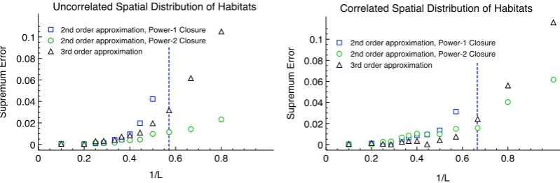
3.4 Numerical Solutions to the Covariance Hierarchy . . . 80
3.4.1 Resolving integrals in the Frequency Domain . . . 81
3.4.2 Results for Gaussian Shaped Transmission Kernel . . . 82
3.4.3 Results for Power-Law Shaped Transmission Kernel . . . 87
3.5 Discussion . . . 91
Chapter 4 Accelerated Simulation for Spatial Epidemics 93 4.1 Introduction . . . 93
4.2 Stochastic Simulation Techniques . . . 95
4.2.1 A Spatial Metapopulation Epidemic Model . . . 95
4.2.2 The Force of Infection as a Spatial Convolution . . . 102
4.2.3 Spectral versus Pseudo-spectral projection . . . 103
4.3 Fast Spectral Rate Recalculation . . . 107
4.4 Numerical Experimentation using FSR method . . . 115
4.4.1 Comparing Simulation Methods by Matching Latent Variables 116 4.4.2 Epidemic Spread amongst Farms . . . 118
4.4.3 Performance of FSR method . . . 119
4.4.4 Geographic Spread of a Plant Disease . . . 126
Chapter 5 Optimal Control of Epidemics using Dynamic
Program-ming 132
5.1 Intervention and Epidemiology . . . 132
5.2 Introduction to Optimal Control Theory . . . 137
5.3 Dynamic Programming . . . 140
5.3.1 Formal Derivation of the Hamilton-Jacobi-Bellman Equation for dynamic programming . . . 141
5.3.2 Classical Solutions to the HJB Equation and Verification The-orems . . . 145
5.4 Optimal Control for the Spatial Epidemic . . . 148
5.4.1 Vaccination and the Controlled Generator . . . 149
5.4.2 The HJB equation for the Spatial Epidemic with Vaccination 154 5.5 Solving the HJB Equation and Optimal Controls . . . 157
5.5.1 Value Iteration for the Embedded Markov Chain . . . 158
5.5.2 Approximate Dynamic Programming . . . 160
5.6 Numerical Examples . . . 168
5.6.1 A Two Area Numerically Solvable Control Problem . . . 169
5.6.2 Pricing the Lack of Information for the Two Area Model . . . 177
5.6.3 Approximately Controlled Epidemics . . . 182
5.7 Discussion . . . 187
Chapter 6 Conclusion and Outlook 190 Appendix A Triple Covariance Dynamics 193 Appendix B Frequency Domain Representation for Higher Order Approximations 196 B.1 The Power-2 Closure . . . 196
B.2 The Third Order Approximation . . . 197
Appendix C Theoretical Basis for Fast Spectral Simulation 201 C.1 Gaussian approximation and the Pseudo-Spectral Projection as a Convolution sum . . . 202
C.2 Convergence of Pseudo-Spectral Approximation . . . 204
C.3 Combined Error and choice of : . . . 212
List of Tables
List of Figures
1.1 A graph in honour of Sir Ronald Ross. . . 6 1.2 Basic SIR model. . . 8 2.1 A schematic diagram of thepossible random times of spread between
two habitats labellediand j. . . 27 2.2 Correlation closure for the Mean-field Epidemic. . . 47 2.3 A spatial epidemic withN = 400. . . 48 2.4 The expected dynamics for the spatial epidemic for a given habitat
distribution. . . 50 2.5 Comparison between simulation and approximation for more local
transmission. . . 51 3.1 Two realisations of the Poisson cluster process. . . 61 3.2 Geometric representation of three population interactions. . . 75 3.3 Moment dynamics for the spatial epidemic with comparison to
co-variance closure results. . . 84 3.4 A comparison of the discrepancy between the 1 closure,
power-2 closure and the third order closure. . . 85 3.5 Dynamics of spatial correlation measure between susceptible and
in-fected populations. . . 86 3.6 The moment dynamics for the spatial epidemic with power-law shaped
transmission kernel and L= 1. . . 88 3.7 The dynamics of the spatial correlation measure between susceptible
and infected populations for the power-law shaped transmission kernel 89 3.8 Epidemic severity for power-law shaped transmission kernels. . . 90 4.1 A schematic diagram of the FSR method. . . 110 4.2 A schematic diagram for effectively imposing non-periodic boundary
4.3 A schematic diagram for Sellke Construction simulation . . . 117 4.4 A comparison of spatial distributions of a slow travelling farm
epi-demic between direct simulation and fast spectral simulation. . . 122 4.5 Results for model of epidemic spread amongst livestock on farms. . 125 4.6 Results for model of disease spread amongst populated plant habitats. 129 5.1 Two population area model. . . 169 5.2 Expected costs for an uncontrolled epidemic and benefit analysis of
a vaccination campaign. . . 174 5.3 Two samples of an optimally controlled epidemic. . . 175 5.4 A cost comparison between optimally controlled epidemics and a
uni-form vaccination policy for symmetric and asymmetric transmission with one initially infected population. . . 178 5.5 A comparison between targeted and untargeted vaccination. . . 180 5.6 The price of early detection. . . 181 5.7 The time-varying probability of the control decision of the exact
Acknowledgments
I would predominantly like to thank my supervisor Matt Keeling for all his guidance over the last few years. I wouldn’t be here without him! Especial thanks go to ev-eryone in the Complexity Science Centre, particularly Jamie, Quentin and Anthony for putting me up at their homes on numerous occasions.
And thanks to everyone in the WIDER research group for continual support and always providing a forum for me to discuss ideas.
Finally, thanks to my wonderful wife who has put up with a lot these past few years, and especially these last few months.
Declarations
This work has been composed by myself and has not been submitted for any other degree or professional qualication.
Abstract
It is now widely acknowledged that spatial structure and hence the spatial posi-tion of host populaposi-tions plays a vital role in the spread of infecposi-tion. In this work I investigate an ensemble of techniques for understanding the stochastic dynamics of spatial and discrete epidemic processes, with especial consideration given to SIR disease dynamics for the Levins-type metapopulation.
Chapter 1
Introduction to Modelling
Infectious Diseases
“The Epidemiologist’s unit is not a single human being, but an aggregate of human
beings”
- Major Greenwood (Greenwood 1935)
1.1
Motivation and Aims
A common feature of the epidemiology of the disease examples mention above is that they areinfectious. Whilst exogenous and environmental factors remain im-portant fundamentally the disease-causing pathogen spreads from host to host each time recruiting a new individual (Human, animal or plant) to the epidemic. It has been recognised at least since the work of Ross, Kermack and McKendrick (Ross 1916; Kermack and McKendrick 1927) in the early twentieth century that the spread of infectious pathogens lent themselves to a mechanistic or model-based interpreta-tion of their progression through time.
The relationship between models written in the language of mathematics and epidemiology has only strengthened since this early pioneering work. When the indi-viduals carrying the infectious pathogen are approximately interchangeable and mix homogeneously amongst themselves then both deterministic and stochastic models for the dynamics of the epidemic have become classical (Bartlett 1956; Bailey 1975; Anderson and May 1992; Diekmann and Heesterbeek 2000; Keeling and Rohani 2008). In this thesis I will be concerned with varying away from this solid theoreti-cal foundation by considering the disease-bearing population as being separated into discrete sub-populations each with a spatial habitat. I will assume more frequent mixing between proximate populations decaying to zero mixing between very dis-tant populations. The assumption of spatially embedded dynamics leads to natural association with concepts of theoretical ecology, in particular the metapopulation concept of local populations in a fragmented landscape (Hanski and Gaggiotti 2004).
1.2
Outline of this Thesis
“Time is what stops everything happening at once. Space is what stops everything
happening to me!”
- John Wheeler
I identify four key properties for a mathematical model of a real-world phenomenon that are important to the theoretical investigator,
• The model should be at least partially theoretically understandable. A model
which represents a ‘black box’ does not promote understanding of the phenom-ena of interest. The investigator should have some theoretical expectation of the generic features of interest, and an idea of what the model is trying to predict. For models of epidemics the expectation of a threshold phenomenon and the concept of the reproductive ratio provide a unifying framework for otherwise rather disparate models of disease.
• The model should be amenable to simulation/numerical solution. For the
mod-ern investigatorin silicomethods have become invaluable for investigating the consequences of model selection beyond the limits of theoretical considerations. For epidemic models even the earliest deterministic models were in a form that required numerical solution. Modern theoretical epidemiology often trades in models involving millions of individuals and which include essential random-ness. Numerical investigation requires large scale Monte Carlo simulation that push the limit of even modern computing resources.
• The model should have understandable feedback properties. Often the goal of
the modeller is not just accurate prediction, but also to use her prediction to guide intervention. For epidemiologists there has been a long history of model-based disease management, with guiding vaccination being a classic example.
• The model should be parametrisable by the available data. Although the
The essential goal of this thesis is to present a tool-box of novel methods for a class of SIR epidemic model that focuses on the spatial properties of disease transmission. For this model I will be tacking the first three model properties listed above. I have left the hugely significant field of appropriate epidemic model parametrisation for future work. In each chapter my arguments and justifications have been given in mathematical form. However, in a number of cases this has only lead to convincing arguments rather than rigorous arguments. My general methodology throughout has been to use the definite underlying mathematical properties of the spatial epi-demic in order to suggest novel applications. In some cases these applications are supported by simulation based evidence rather than proper mathematical rigour, which remains future work. I feel it is important to make this clear to the reader.
Inchapter 2I will review some theoretical results from the calculus of pure jump processes, in particular the form of Itˆo lemma (a chain rule for stochastic pro-cesses) for pure jump processes. I will also introduce the basic spatial and stochastic model that I will then use throughout the rest of this work. The basic spatial model will be shown to admit representation as a jump process with an explicit stochastic differential equation (SDE) formulation. This formulation will be exploited in order to give a set of ODEs approximating the expected dynamics of the spatial epidemic.
In chapter 3the stochastic differential model for the spatial epidemic will be extended to include the case where the spatial locations of the habitats are them-selves random variables. I use the classic approach of spatial moment equations to investigate the interplay between the stochastic dynamics of the infectious disease and the random, possibly spatially clustered, environment of habitat locations. The novelty of my approach lies in building the moment equations directly from the stochastic microscopic dynamics, which leads to a slightly corrected version of the moment equations compared to some extant in the literature. I will also give a theoretical and numerical investigation into the performance of different types of ‘closing’ approximations for the moment equation I derive.
of a novel simulation algorithm tailored to the spatial epidemic which has excellent numerical efficiency compared to traditional stochastic simulations techniques as the population size grows large.
Finally, in chapter 5 I will review the classic dynamic programming ap-proach to solving continuous-time or multi-stage decision problems. I will introduce an optimal vaccination scheduling problem and demonstrate that for certain scenar-ios the space of optimal vaccination actions at any time is dramatically reduced to a small set. I will solve the optimal control problem to numerical exactness for toy problem, with a focus on the effect on optimality of the vaccinating agency lacking information about the epidemic. I also introduce a novel method for approximately solving optimal vaccination problems for the spatial epidemic, inspired by the field of approximate dynamic programming. I will demonstrate this method on an epi-demic of sufficient size that classical dynamic programming would be numerically infeasible.
1.3
Historical context and the SIR model of Disease
“... the principal problems of epidemiology on which preventive measures largely
depend, such as the rate of infection, the frequency of outbreaks, and the loss of
im-munity, can scarely ever be resolved by any other methods than those of analysis.”
- Sir Ronald Ross 1916 (Ross 1916).
Ross1 in his ground breaking work on the population level dynamics of infectious
diseases, or pathometry in his terminology, expressed his surprise at the dearth of mechanistic a priori methodology for the study of infectious diseases. His solution to this lack was to develop what he referred to as the ‘theory of happenings’; that the incremental change in the population levels of the ‘affected part’ and the ‘un-affected part’ over a short time interval are proportional to a rate and the size of the time interval. The rates he conceived were nativity, mortality, immigration and emigration for the overall population and for the disease dynamics a ‘happening element’ and a ‘reversion element’, which would now be referred to as respectively as transmission rate and recovery rate. Ross also embarked on a discussion of the type of recursion; whether the reverting individuals had gained long-term immunity
1Second noble prize winner in Physiology and Medicine (1902) for the identification of the
to subsequent infection or if immunity was waning and whether they were capable of spreading further infection after reversion.
0 20 40 60 80 100 120 140 160
Time (days) 0
1000 2000 3000 4000 5000 6000
Af
fe
ct
e
d
Pa
rt
o
f
th
e
p
o
p
u
la
ti
o
n
Pathometry Infection Curve from the "Theory of Happenings"
Figure 1.1: A graph in honour of Sir Ronald Ross. The numerical solution to the epidemic curve (infecteds number) according to his theory of happenings for when reversion (recovery) gives
permanent immunity (SIR model) and there are no demographic effects. Population size is 105,
the rate of happenings (transmission rate) is 0.375×10⁻⁵×number of unaffected (susceptibles)×
number of affected (infecteds) per day. The reversion rate (recovery) is 0.25×number of affected
per day.
In this seminal work Ross identified the cessation of disease outbreak with the depletion of susceptible individuals available for sustaining the epidemic, a contro-versial concept at that time. He also found that the growth of numbers of infectious individuals would be exponential before this depletion effect took hold leading to an ‘epidemic curve’ that is almost symmetrical but somewhat heavier tailed at the end of the epidemic. These observations, which have now become standard, were revolutionary in the early 20th century since they demonstrated that a plausible model of human interaction and population dynamics could, by themselves, explain the intermittency of the epidemics that plague mankind. This has become a stan-dard concept for the theoretical community of epidemiologists but was completely rejected at the time in certain sections (Brownlee 1909), where time-varying bio-logical factors were favoured such as the pathogen losing infectiousness over time. Ross’ differential model (Ross 1916) was ,
dP = (n−m+i−e)Adt+ (N−M+I−E)Zdt, (1.1)
dA = (n−m+i−e−h)Adt+ (N +r)Zdt, (1.2)
Where P, A and Z are respectively the population size, number of not affected (susceptible individual) and the number of affected (infectious individuals). n, m, i, e
parameterise the nativity, mortality, immigration and emigration demographic rates for the susceptibles and their capital versions for the infecteds. h is the rate of happenings (recruitment rate of new infecteds) andr is the reversion rate (recovery rate) where the reversion here is back into the susceptible class. In honour of Ross’ fundamental contribution I give a numerical solution to his theory of happenings for epidemics assuming permanent immunity reversion. The solution would have been a considerable numerical challenge in 1916, but is trivial with modern computing resource (figure 1.1).
1.3.1 Transmission and the Deterministic SIR Model
The next major contribution was from Kermack and McKendrick (Kermack and McKendrick 1927) who explored the differential model of epidemics from the per-spective of transmissibility; that the recruitment of new infecteds was due to the infectiousness of the current infecteds, which mix homogeneously amongst the total population, a mass action assumption (Isham 2005). They left their model rather general, allowing the recruitment rate of new infecteds at each time to depend on the prior history of susceptible numbers leading back to the origin of the epidemic. Individuals recovering from the disease were assumed to have long lasting immu-nity and to play no further role (figure 1.2). There has been some interest in the general model (Fraser 2007) but their classic contribution was the special case now known as the susceptible-infected-removed (SIR) model of disease (Kermack and McKendrick 1927; Bartlett 1956; Bailey 1975; Anderson and May 1992; Diekmann and Heesterbeek 2000; Keeling and Rohani 2008), given by the following simple non-linear ordinary differential equation,
d
dtS(t) = −
β
NS(t)I(t), (1.4) d
dtI(t) = β
NS(t)I(t)−γI(t), (1.5) d
dtR(t) = γI(t). (1.6)
depen-dent2 transmission (Grassly and Fraser 2008). The assumption behind frequency dependent transmission is that each individual has an expected number of contacts per fixed time interval that does not depend on the total population size N, see (Diekmann and Heesterbeek 2000) chapter 10 for a more general discussion on in-fectious contacts. The solution given in figure 1.1 is for the SIR model choice as a specialisation of Ross’ equations.
There are some immediate consequences of the basicSIRmodel, firstly that the total number of individuals N = S +I +R is conserved, since there are no demographic effects considered in the model therefore R(t) =N −S(t)−I(t) can be dropped. For the epidemic state (S(t), I(t)) = (S0, I0) the number of infectious individuals is growing if, and only if,
S0 N >
γ
β =
1
R0
. (1.7)
This gives a condition for the number of infecteds to be growing in terms of a new quantity,R0=β/γ.
Recovery
Secondary Infection
[image:20.595.205.427.405.596.2]Recovereds are immune
Transmission
Figure 1.2: The basic SIR epidemic model. The two dynamical transitions are for currently infectious individuals (red box outline) to recruit susceptible individuals (green box outline) as their secondary cases and for infectious individuals to recover and become removed from the epidemic (blue box outline).
2Rather confusingly the alternative without the 1/Nscaling is often referred to in epidemiological
Thereproductive ratio R03 is one of the most important and robust
quanti-ties in epidemiology; it is written in terms of the transmission and recovery rates and hence is a measure for both the biological infectiousness and persistence of the infectious disease and the underlying mixing between infectious and susceptible indi-viduals. R0 governs the important threshold phenomenon known asherd immunity
(Anderson and May 1985a; Fine 1993). Herd immunity is a direct consequence of (1.7) that an infectious disease can only recruit growing numbers of individuals if its reproductive ratio is greater than the inverse population density of susceptibles. This simple observation is crucial since it gives the threshold proportion, denoted
V∗, of the population that must be made removed by some method, in most cases by a vaccination campaign, in order to incur herd immunityfor the entire population
as,
V∗= maxn0,1− 1 R0
o
. (1.8)
Equation (1.8) is fundamental, the entire population can be effectively protected from an infectious disease by directly protecting just a fraction of the population since whatever (typically small) numbers of initial infecteds seed the epidemic will inevitably decline leading to a small outbreak. IfR0 <1 then the infectious disease cannot invade even a naive4 population. By contrast without vaccination the
num-ber of infecteds increases until the susceptibles are sufficiently depleted that (1.7) no longer holds which leads to a large epidemic.
1.3.2 Discrete and Stochastic Epidemic Models
So far in this introduction I have consistently referred to individuals but only dis-cussed classical models that are deterministic and written in terms of ordinary dif-ferential equations (ODE). A model that predicts a non-integer population number of susceptibles and infecteds requires some further interpretation. Enforcing the dis-creteness of the SIR model has historically been done in conjunction with introducing randomness or stochasticity into the transmission and recovery of individuals for a continuous time model (Bailey 1950; Bartlett 1956; Bartlett 1960a; Bailey 1975), a discrete time model such as the Reed-Frost chain binomial model (Becker 1989) or
3
Not to be confused notationally with R(0), the initial number of removed individuals. 4
An (immunologically naive population is one in which every individual, bar the initial set of
agenerational time5 model such as a branching process (Griffiths 1973).
The ‘work horse’ of random models for the SIR process is the stochastic con-struction where each individual upon being recruited to the infected class remains infectious for the random length of timeT, called the infectious duration (Conlan et al. 2010). During that time the infectious individual makes random infectious con-tacts, the standard model being contact at the points of a Poisson process (Ball and Neal 2002), with the rest of the population. When a susceptible is contacted that individual is recruited to the infectious class. The most popular choice is to have the infectious durations exponentially distributed since the stochastic epidemic con-struction with Poisson process contacts and exponential durations can be described as a Markov process (Ethier and Kurtz 1986) with transition probabilities given by the intensity of the Poisson contactβ/N and the rate parameter of the exponential duration timeγ,
P[(S, I)(t+h)−(S, I)(t) = (−1,1)|(S, I)(t)] = S(t)β
NI(t)h+o(h), (1.9) P[(S, I)(t+h)−(S, I)(t) = (0,−1)|(S, I)(t)] = γI(t)h+o(h). (1.10)
Where (S, I)(t) describes the random numbers of respectively susceptibles and in-fecteds at timet.
A major departure for the theory of the stochastic SIR epidemics compared to its deterministic counterpart is that due to randomness the threshold phenomenon is given a probabilistic interpretation in terms of infinite sized populations. IfZN(∞) denotes the final number of cases6 for a population of size N then the probability
of a ‘true epidemic’ (Ball 1983) is said to be,
P(( lim
N→∞ZN(∞)) =∞). (1.11)
This is best interpreted as a probability of a non-zero fraction of a large popula-tion becoming infected (i.e. a significant epidemic occurring) with the other oppopula-tion being that an effectively zero fraction of a large population becomes infected (i.e. a small epidemic occurring). The probabilistic version of the threshold effect for the stochastic epidemic with dynamics given by is that for an initial population density of susceptibless0 =S(0)/N and an initial number of infecteds I0 then the
5
The generation of an infected individual is the number of infection events she is removed from the initial set of infecteds (the 0th generation).
6
probability of a significant epidemic is (Ball 1983),
P(Significant sized epidemic) = 1−
minn1, 1 s0R0
oI0
. (1.12)
The threshold vaccination coverage given by (1.8) can be reinterpreted for the stochastic SIR model as the minimum vaccination coverage that that makes the probability of a significant or ‘true’ epidemic zero. On other side of (1.12) is that even if the critical vaccination coverage (1.8) is not reached, or if vaccine has not been attempted, there is a probability that a small number initial infecteds will fail to cause a significant sized epidemic. This is not a feature of the determin-istic SIR model, where the numbers of infected individuals always increases when
S(t)/R0 < 1. This bimodal character, i.e. large or small outbreaks, or U-shape
(Isham 2005), of the distribution of epidemic final sizes is a classic feature of the stochastic SIR model. Even for diseases with SIR-type epidemiology for the in-dividual but that persist for long periods of times due to recruitment of newly arriving susceptible individuals7 (Anderson and May 1992), such as measles
(Gren-fell, Bjørnstad, and Kappey 2001; Jansen 2003), stochastic fluctuations can bring about population level ‘fade-out’ (Bartlett 1960b; Nasell 1999).
Given the above considerations, as a first approximation, the modeller would expect the average disease progression for a stochastic SIR model to be decreased from the deterministic model. More formally, the expected rate of recruitment of new infectious individuals is given as,
d dtE[I] =
β
NE[S]E[I]−γE[I] + β
Ncov[S, I]. (1.13)
Wherecov[S, I] is the time varying covariance between the random numbers of sus-ceptibles and individuals (Keeling 2000; Herbert and Isham 2000; Isham 2005). The basic SIR model this covariation will be negatively signed leading to, on average, retarded growth of infected numbers compared to the deterministic model. However this is not a universal effect, the interplay between stochasticity and an oscillatory approach to equilibrium for the SIR model with demography can lead stochastic resonance and wild oscillations in disease burden, for a more detailed discussion on stochastic amplification for disease models with demography see (Alonso, McKane, and Pascual 2007).
7
Since both the deterministic and stochastic SIR models have been extensively used for both the theoretical and practical understanding of the risk and dynamics of infectious disease it has been of interest to rigorously establish the link between the models. Kurtz established conditions for the convergence of Markovian dynamics with a state space of natural numbers with some maximum size N, say X(t), to deterministic processes in density x(t) = X(t)/N as the maximum size diverges
N → ∞; a variety of central limit result for Markov processes (Kurtz 1970; Kurtz 1971), which has now been further generalised, c.f. (Kallenberg 2002) theorem 17.15. Specialising Kurtz’s results to the stochastic SIR epidemic gives convergence conditions,
β(N)S(t)I(t)∼ O(N), t≥0 “Density dependence”, S(0)
N →s0,
I(0)
N →i0, Convergence of initial condition.
Where I have denoted the intensity of the individual to individual (Poisson) con-tact process β(N) in order to emphasise that, in principle, the contact intensity’s dependence on population size is a model choice. The standard choiceβ(N) =β/N
whereβ is a constant satisfies the density dependence criterion.
If the convergence conditions are satisfied then as the total population size diverges N → ∞, the density SIR process s(t) =S(t)/N, i(t) =I(t)/N converges8
onto the deterministic density SIR process,
d
dts(t) = −βsi, (1.14)
d
dti(t) = βsi−γi, (1.15)
s(0) =s0, i(0) =i0. (1.16)
The standard SIR models given above were formulated in terms of identical and homogeneously mixing host individuals under-going epidemic invasion. This gives a solid theoretical foundation, however in light of real-life epidemic examples often the epidemic model must be modified in order to explain and predict observed phenomena. Examples of heterogeneity that have been incorporated into epidemic models include multi-pathogen models such as for malaria where it has been shown that treating different malaria strains as interchangeable can be mis-leading (Gupta,
8
Swinton, and Anderson 1994). Age structured models have been shown to be par-ticularly important in understanding childhood diseases (Anderson and May 1983); is due to both the epidemic sustaining itself by recruiting the individuals born in to the susceptible compartment and the heterogenous mixing between age-groups for human populations, which has been empirically verified (Mossong et al. 2008). Keeling and Rohani (Keeling and Rohani 2008) give large numbers of examples of further host and pathogen heterogeneities and appropriate model extensions.
The heterogeneity I will focus on in this thesis will be spatial heterogeneity. The transmission of a infectious disease between individuals often occurs at close proximity, with long range spreading in a population due to individual movement. However, realistically representing individual movement in a model can be difficult, not to mention leading to analytic intractability and problematic parametrisation. Nonetheless, the habitat location of individuals, e.g. households or farms, are often known and in conjunction with assumptions and arguments on the mixing pattern of the population one can hope to capture disease dynamics as the spatial spread on these sessile locations. Moreover, in the case of plant diseases the individual is stationary and disease transmission is inherently long-range, e.g. via wind-borne dispersal of fungal spores. In this case the individual and the ’habitat’ can be directly associated with one another.
1.3.3 Spatial Epidemic Transmission and the Metapopulation Model
There are several approaches to modelling the dynamics of the spread of spatial infection, including PDE models (Murray, Stanley, and Brown 1986) and agent-based models (Barrett et al. 2008), but themetapopulation model is often the preferred formulation due to its relative simplicity and flexibility. The metapopula-tion model consists of discrete point habitats in continuous space that can interact with each other. Its origins date back over 40 years (Levins 1969), but it is experienc-ing increasexperienc-ing use in a wide number of problems in population dynamics (Hanski and Gilpin 1997; Hanski and Gaggiotti 2004). While the original metapopulation model assumed an equal rate of interaction between all habitats, the inclusion of more real-istic rates that decay with spatial separation has lead to a greater understanding of the roles of spatial structure, with applications in as diverse settings as population biology (Ovaskainen and Cornell 2006a; Cornell and Ovaskainen 2008), conservation biology (Hanski), evolutionary biology (Heino and Hanski 2001) and epidemiology (Gibson 1997; Lloyd and Jansen 2004; Grenfell, Bolker, and Kleczkowski 1995).
Chapter 2
A Spatial and Stochastic
Epidemic Metapopulation
Model
2.1
Introduction
The aim of this chapter is to incorporate stochastic transmission and spatial frag-mentation into the general framework of theSIRcompartmental model with a view to the analysis and understanding of their interplaying effect on disease invasion and the final burden of the epidemic. I will treat the time-varying risk of disease intro-duction to each naive population as Markovian; that is that the probabilistic rate of recruitment to the infectious class will depend only the current spatial distribution of infectious populations. I will exploit the assumed Markovian nature of the model in order to represent the epidemic dynamics as stochastic differential equations (SDE) driven by a set of Poisson processes.
Itˆo lemma1 (Ito 1951; Oksendal 2004) result which allows functions of diffusion
pro-cesses to be represented as diffusions themselves.
In this chapter the stochastic dynamics of the spatial epidemic will be anal-ysed using the tools of stochastic calculus for processes which evolve in time only in jumps (Bichteler 2002; Klebaner 2005). Compared to diffusion models the sample paths of a pure jump process are constant except at the arrival of discrete points e.g. infectious transmission or recovery events; whereas nearly all diffusion sample pathes are sufficiently rough as to be nowhere differentiable by contrast the sample paths of pure jump process are nearly everywhere differentiable. This profoundly simplifies the integration theory for pure jump processes. Moreover, an Itˆo lemma remains accessible in a particularly simple form.
The goal will be to construct systems of ODEs where each deterministically evolving variable approximates a statistical quantity of interest, for example the expected burden of infectious individuals in a population at a certain time. In prin-ciple such a construction allows the investigator to analyse the expected behaviour of an epidemic according to a model that incorporates randomness and the fun-damental discreteness of individuals within a population using the tools familiar from the theory of ODEs. The system of ODEs which approximates the dynamic moments and evolving covariances of the random epidemic is constructed by sequen-tially representing the stochastic dynamics of increasing product chains of disease state indicator functions, which I dub thedynamical hierarchy of the epidemic pro-cess.
I will first review some results for pure jump processes that will be useful in the sequel. I will then introduce the fundamental model of epidemic spread amongst a spatial metapopulation that I use throughout this work. The fundamental model will be shown to be equivalent to a pure jump process represented in a Stochastic differential equation (SDE) form which is amenable to analysis; the covariances be-tween stochastic disease states at different populations is found to obey a hierarchy of ordinary differential equations which can be derived from the SDE formulation.
I am able to bound the size of the population disease state covariances driving the deviation between the expected dynamics of the stochastic model and related deterministic models in terms of an inverse length scale of disease transmission
1
in a manner closely reminiscent of results found in theoretical population biology (Ovaskainen and Cornell 2006b). This allows the theory to be consider asymptoti-cally exact, in the sense that it has the same limit property as the basic frequency dependent SIR model, albeit here both a large population limit and a diverging length scale of transmission are required.
2.2
Stochastic Calculus with Jumps
In this section I give a brief introduction to stochastic calculus for processes that change only in discrete jumps. The rather beautiful theory of diffusion processes is not relevant for the understanding of disease models where events occur discretely - I will only be concerned with models where an individual or population are con-sidered to become infectious at a certain time in one ‘jump’.
If I was considering a deterministic model of disease the natural first step in analysis would be to write the dynamics of the disease processX= (X(t), t≥0) in a differential form,
dX(t) =F(X(t))dt. (2.1)
The taxonomy of this equation is that infinitesimal change in timedt(the integrator) drives the infinitesimal evolution of the temporal disease statedXthrough the vector field at that time F(X(t)) (the integrand). The aim of this section is to establish a meaningful way of writing the dynamics of the stochastic jump model of disease transmission in an analogous differential form, and then harvest the useful theory that exists around such processes. The difficulty compared to classical calculus is that the driver of the differential equation won’t be time, leading back to well understood classical calculus, but rather a set of discrete processes. The differential model will be in the form,
dX(t) = (F(X(t)), dN(t)). (2.2)
associated jump sizes{(τ(n), Z(n))}
n∈N, giving the sample path,
N(t) =N(0) +X n∈N
1(τ(n)≤t)Z(n). (2.3)
Where1(·) is the standard boolean indicator function. Each sample path of a pure jump process is c`adl`ag2. The restriction on pure jump processes to all jump sizes {Z(n)= 1}
n∈N withN(0) is called a counting process that is that,
N(0) = 0, N(t) =X n∈N
1(τ(n)≤t). (2.4)
Defines the sample path of a counting process for some set of hitting times{τ(n)}
n∈N.
In the following I cover a set of results that will be useful for analysing the behaviour of differential models driven by counting processes; the exposition is based upon (Applebaum 2004; Klebaner 2005; Di Nunno, Øksendal, and Proske 2009).
A stochastic processesX = (X(t), t≥0) is a collection of random variables,
X(t) indexed by the time processt. Each random variable is a measurable map from a probability space to a state space which assigns a value to each sample element of the probability space, I will restrict to real multi-dimensional process so that the state space is Rn endowed with the standard Borelσ-algebra. The probability
space is given as the triple (Ω,F,P) where Ω is the set of all possible samples for
the stochastic model. F is a collection of sub-sets of Ω which define all events that can be assigned a probability within the model; by necessity F is endowed with the algebraic structure of a σ-algebra. It is worth mentioning that F is as much a model choice as the other elements, restrictingF is equivalent to restricting the information accessible to an observer. P is a probability measure P : F → [0,1].
In addition, I define a filtration3 (F
t)t≥0 on (Ω,F). A stochastic processX which
is Ft-measurable for t ≥ 0 is called adapted. Whereas F represents all observable events for X, the filtration represents all information up to timet. Unless stated oth-erwise I use aσ-algebra which contains the complete information about the driving counting processes, i.e. all hitting times for the chosen sample element ω∈Ω, and a filtration that contains this information up until each time t. This is called the natural filtration of the counting processes. Notationally, I follow the majority of
2
A sample pathN(t) is said to be c`adl`ag if limu↓tN(u) = N(t) and limu↑tN(u) exists fort≥0.
3A filtration is an increasing family of σ-algebras which models the expanding information
authors on stochastic processes and writeX(t, ω) =X(t), t≥0, ω ∈Ω, suppressing explicit dependence of the process on the sample.
A condition for defining ‘sensible’ (i.e. non-anticipatory) processes is if the integrand formally introduced in (2.2) can be completely determined by knowing only the events leading up to each time t. In other words if the instantaneously current or future random behaviour of the integratorN(u) at timesu≥tdoes not influence the integrand F(X(t)) at time t. This causal property is guaranteed by restricting F(X(t)) to be a predictable process. For my purpose it is sufficient to define a sub-class of predictable processes,
Definition 2.2.1. The process X is a predictableprocess if X is left-continuous and adapted.
Of crucial importance will be the ability to split processes into a
compen-satorprocess, which governs the drift of the process, and a local4martingale process,
which can be thought of as the fluctuations around the drift. This is referred to in the literature as thesemi-martingale representation, but I find drift and fluctu-ation more explanatory and use that terminology. The martingale property for the ‘fluctuation’ part of the stochastic process will be crucial.
Definition 2.2.2. An adapted stochastic processM(t) is a martingale if • E[|M(t)|]<∞ for t≥0.
• E[M(t)|Fs] =M(s) almost sure for 0≤s < t <∞.
A martingale is said to be square integrable if also supt≥0E[M2(t)]<∞.
For the ‘drift’ part of the stochastic process, the compensator, I restrict my definition to include only the examples useful for this work,
Definition 2.2.3. The compensator A(t) for a counting process N(t) is the unique
predictable process such that N˜(t) =N(t)−A(t) is a local martingale.
For the drift and fluctuation decomposition used in this work I will use,
X(t) =X(0) +A(t) + ˜X(t), (2.5)
A(0) = ˜X(0) = 0.
4A property for a stochastic process X is said to be local or to hold locally if there exists a
Hence, an expectation taken on the fluctuation martingale process ˜X(t) returns zero. This also explains the notation A(t) for the compensator; it refers to the addition to the initial stateX(0).
I will be concerned with counting processes N(t) where the events arrive at some deterministic average rate5 ν(t) defined by the compensator,
A(t) =
Z t
0
ν(s)ds, t≥0.
Counting processes with deterministic and continuous compensators can be com-pletely characterised as Poisson processes ((Klebaner 2005) Theorem 9.9),
Theorem 2.2.1. LetN(t)be a counting process with continuous deterministic
com-pensatorA(t). Then it has independent Poisson distributed increments such that,
(N(t)−N(s))∼P oisson(A(t)−A(s)), 0≤s < t. (2.6)
Theorem 2.2.1 will be of great use in the sequel. I will henceforth refer to the driving counting processes as the driving Poisson processes. The local martingale
˜
N(t) =N(t)−A(t) is called the compensated Poisson process.
Having established the Poisson character of the discrete processes which will play the role of the driver or integrator, I turn to defining the meaning of the differential model (2.2). I am restricting to one dimension and one Poisson driver for simplicity, multidimensional processes with many independent Poisson drivers extend naturally in ‘inner product’ form. For some vector field F : Rn → Rn and
the one-dimensional Poisson processN(t) we define the process X such that,
X(T) =X(0) +
Z T
0
F(X(t))dN(t). (2.7)
The integral on the right hand side of (2.7) is astochastic integral, which is a random variable defined as a limit in probability6,
Z T
0
F(X(t))dN(t) = lim n→∞
X
ti∈πn
F(X(ti))(N(ti+1)−N(ti)). (2.8)
5
Often referred to as thestochastic intensity of the counting process. 6
A sequence of random variables {Xn}n≥0 is said to converge in probability to a limit (in
Where (πn)n≥0 is a sequence of ordered partitionsπn= (t0= 0, t1, . . . , tn−1, tn=T) of the interval [0, T] with vanishing mesh separation. If this limit exists then,
dX(t) =F(X(t))dN(t), (2.9)
is the differential form of (2.7) with unique (in probability) solution X(t), t ≥
0. Stochastic integration where the integrator is a Poisson process is considerably simpler than for the case where the integrator is a Brownian motion. For a Poisson integrator selectingω∈Ω specifies the set of hitting times and (2.8) gives,
Z T
0
F(X(t, ω))dN(t, ω) =X n∈N
1(τ(n)< T)F(X(τ(n), ω)). (2.10)
Where the integral has been interpreted as a Stieltjes integral (see (Klebaner 2005) chapter 1) completely determined by the choice of sample element ω ∈ Ω. This is analogous to the graphical construction of the contact process (c.f. (Liggett 1985)) and the Poisson hitting construction for the stochastic SIR epidemic (see (Ball and Neal 2002) and later in this chapter). Equation (2.10) also demonstrates directly from the definition (2.8) that stochastic processes driven by counting processes are pure jump processes with hitting times given by the integrator process and jump sizes given by the integrand process. For stochastic processes driven by Brownian motions this direct definition from the sample element turns out to be impossible, c.f. (Applebaum 2004) chapter 4. I state a classical existence theorem (c.f. (Di Nunno, Øksendal, and Proske 2009) chapter 9) for stochastic integrals, albeit restricted to Poisson process integrators and one dimension.
Theorem 2.2.2. Let N = (N(t), t ≥0) be a Poisson process of intensity ν(t), let
F(t) be a predictable process. If
E
h Z T
0
(|F(t)|+F2(t))ν(t)dti<∞, T >0,
then the stochastic integral,
X(0) +
Z T
0
F(t)dN(t),
exists and is called the solution to the stochastic differential equation (SDE) (2.9).
Moreover, the process
˜
X(T) =
Z T
is a square integrable martingale.
The usefulness of theorem 2.2.2 is not just that it guarantees that a process
X(t) driven by Poisson processes satisfying the conditions above will not ‘disappear’ to infinity but also that the stochastic integral with respect to the compensated Pois-son process is itself a martingale. Therefore, given a stochastic differential model one is able not only to split the integrator into drift and fluctuation form but also the whole process.
Finally, there is an Itˆo formula for pure jump processes (c.f. (Klebaner 2005) chapter 9) that will be very useful in the sequel for calculating the stochastic rate at which epidemic states jointly vary in time. Given any pure jump processX the Itˆo formula for pure jump processes allows one to define a new pure jump process for each locally bounded functionf.
Theorem 2.2.3. The pure jump Itˆo formula. Let X = (X(t), t ≥ 0), be
an N-dimensional stochastic process driven by a set of counting processes N(t) =
(N1(t), . . . , Nn(t))T,
X(t) =X(0) +
Z t
0
F(X(s))dN(s).
For some set of predictable processes depending on X in matrix form F(X(t)) =
(Fij(X(t)))1≤i≤N,1≤j≤n. Let f :RN →Rbe locally bounded and define
Y(t) :=f(X(t)), t≥0.
Then the processY = (Y(t), t≥0)is a one-dimensional pure jump stochatic process
and its differential form is given by
dY(t) = n
X
j=1
[f(X(t) +Fj(X(t)))−f(X(t))]dNj(t)
where Fj(X(t)) is the column numberj of theN ×n matrix F(X(t)).
2.3
The Spatial and Stochastic Epidemic Model
from population to population as only depending on spatial distance between the habitats of the populations modulated by a transmission kernel. The basic model form is equivalent to a stochastic process driven by Poisson processes.
2.3.1 Epidemic Dynamics
The population undergoing epidemic invasion is considered to be distributed between a discrete set ofN habitats labelled i= 1, . . . , N. Each habitat is considered to be interchangeable and to have effective area zero compared to the background space; ergo the only information about the habitats required for this epidemic model is their spatial co-ordinates, {xi}Ni=1. When considering a finite number of habitats
the spatial co-ordinates are constrained to be within a d-dimensional box of side lengthl,A= [−l/2, l/2]d. The density of habitats in the space is given byN l−d; in this work I choose units such that the spatial density of habitats is 1 i.e.
N l−d= 1. (2.11)
Whenever a limitN → ∞is considered, implicit is also a limitl→ ∞taken in such a manner as to maintain the unity of the spatial density. This choice of units has the benefit of removing habitat spatial density as an unnecessary parameter from the model. Moreover, it allows the definition of a natural length scale, i.e. the units in which (2.11) holds, useful for the comparison of theoretical predictions to field data.
In order to model the spatiotemporal development of an invasive pathogen spreading from population to population I assign a disease state to each population. Each populationi, in addition to a spatial locationxi for its habitat, is assigned a stateσi(t)∈ {S, I, R} according to the classic SIR compartmental model of disease (Kermack and McKendrick 1927; Bartlett 1956). The state is considered to repre-sent the entire population abiding at habitat i; this is a modelling choice that is appropriate when intra-population transmission occurs at a much faster time scale than inter-population transmission, in particular subsequent transmission is consid-ered to have negligible effect on the population subsequent to initial introduction of the pathogen. Treating the host population as a single host individual conforms to the standard Levins-type metapopulation (Levins 1969). The initial disease state
A Spatial Transmission Model
I now give the details of the stochastic transmission model between populations abiding in the spatially fragmented meta-population. Central to this work is that each infectious (I) population introduces a risk per unit time of causing transmis-sion to each susceptible (S) population. Each source of epidemic risk represents a coarse graining over all possible realistic routes of infection. Examples of transmis-sion pathways might be the roaming of Badger individuals between cattle farm as a potential transmission pathway for bTB(Donnelly et al. 2005; Vial, Johnston, and Donnelly 2011) or the movement of potentially infectious livestock to a farm with a naive population (Vernon and Keeling 2009). Each transmission risk is assumed to operate independently of other sources with the consequence that the probabilistic rate of disease establishing itself in a susceptible population is the summed risk of transmission per unit time over the set of infectious populations.
The rate at which an infectious population introduces the pathogen into a susceptible population is modulated by their spatial separation. The modulation is governed by thetransmission kernel K. Investigating the functional dependence of the epidemic dynamics on the choice of transmission kernel is one of the main goals of this work. I impose conditions on the selection of the spatial kernel:
• K is a smooth function on Rd.
• The transmission is spatially isotropic and radially symmetric i.e. K(x) ≡ K(|x|) ∀x∈Rd.
• K is a decreasing function of|x|with a maximum atK(0) (if it exists).
• There exists a characteristic length scaleLto transmission, which is indepen-dent of the shape of the transmission kernel. To be exact I require thatK is in the formK(x) = L1dk(x/L) for some shape functionk independent ofL.
The final condition gives that the total ‘effort’ of the infection over space, defined as,
K0 =
Z
A
K(x)dx, (2.12)
popu-lation dynamics (Kurtz 1970; Kurtz 1971).
Almost surely each infectious population remains infectious, and thereby con-tributing to the ongoing epidemic, for a finite period of time. In this model once a population has ceased being infectious it is removed (R) from the epidemic dy-namics, no subsequent re-infection can occur. The recovery mechanism potentially models either the population reaching a critical herd immunity (Anderson and May 1985a) after which infection declines rapidly, detection and population removal as is commonly the case with diseases of commercial livestock (Ferguson, Donnelly, and Anderson 2001b) or even the complete elimination of host by the disease as is the case with certain diseases of plants (Rizzo and Garbelotto 2003). Recovery oc-curs at a constant probabilistic rateγ during the infectious period of the population.
The model considerations above point towards the definition of Markovian dynamics for the symbolic processσ= (σ(t) = (σ1(t), . . . , σN(t)), t≥0) on{S, I, R}N with initial law,P0 and probabilistic dynamics specified by,
P(σi(t+h) =I|σ(t), σi(t) =S) =
h X
j:σj(t)=I
K(xi−xj)
i
h+o(h), (2.13)
P(σi(t+h) =R|σi(t) =I) =γh+o(h). (2.14)
i= 1, . . . , N, h >0.
This version of defining Markovian dynamics is possibly the most natural since one can consider the stochastic rates of new events arriving as setting the probability of a discrete disease event, either an infection or recovery event, arriving in the infinitesimal future interval [t, t+ dt]. The probability of more than one event occurring simultaneously is zero; an event either occurs in the infinitesimal future or it doesn’t.
2.3.2 An Equivalent Stochastic Model
Firstly, I define N2 independent Poisson processes, using the notation X ∼ P P(ν) to indicate thatX is a Poisson process of intensity ν.
NI
ij ∼P P(K(xi−xj)), i, j = 1, . . . , N, i6=j, (2.15)
NiR∼P P(γ), i= 1, . . . , N. (2.16)
The spatial epidemic dynamics can now be subordinated to these Poisson processes. This is a technique that is common amongst the community of applied probabilists working in the field of mathematical epidemiology (Ball and Neal 2002) in order to better analyse thresholds for epidemic eradication (Ball, Britton, and Lyne 2004) or the probability of early extinction and distribution of final epidemic sizes (Ball, Sirl, and Trapman 2010). The essential idea is that the number of jumps of a homo-geneous Poisson process P P(ν) on the time interval [t, t+h) is always distributed as Poisson(νh) due to stationary independent increments. Hence, the probability of the number of jumps being≥1 is
1−P(#jumps∈[t, t+h) = 0) = 1−e−νh =νh+o(h).
Similarly forM independent homogenous Poisson processes each with some intensity
{νi}Mi=1 the probability of there being no jumps for any of the M processes is
1−P(#jumps∈[t, t+h) = 0) = 1−
M
Y
i=1
e−νih=
M
X
i=1
νih+o(h).
These basic considerations demonstrate that probabilistic dynamics of the form (2.13) and (2.14) can be constructed using the hitting times for jumps of judiciously chosen Poisson processes.
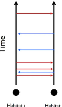
I now give a mechanistic description of constructing a sample epidemic from Poisson processes. An initial stateσ(0) is drawn from P0. The hitting times of the
Poisson processes form the complete set of times at which events can occur, the set of Poisson processes{NI
ij}defining the possible times of populationibecoming infected by populationj and {NR
i } defining the possible times of recovery for populationi. The dynamics evolve thus, with a pictorial desciption being given in figure 2.1:
1. Generate a sufficiently large number of hitting times for each Poisson process,
{(τI
ij)(n)}n≥0 and {(τiR)(n)}n≥0 and set time t= 0.
3. Sequentially, from the earliest hitting time onwards, check which Poisson pro-cess originated the hitting time. If the originator of the current hitting time
τ(n) wasNI
ij and an infectious transmission is feasible, that is that population
i is susceptible and population j is infectious, then update the time to τ(n)
and the local state at populationitoσi(τ(n)) =I. Similarly, for hitting times originating fromNR
i where the feasibility is given by populationibeing in the infectious state and update is given by σ(τ(n)) = R. At all other times the
epidemic state is constant.
[image:39.595.265.368.321.497.2]4. Ifσi 6=I for all i= 1, . . . N. Then terminate the dynamics.
Figure 2.1: A schematic diagram of the possible random times of spread between two
habi-tats labelledi andj. The red arrows indicate the hitting times of the Poisson process NI
ij(t) ∼ P P(K(xi−xj)). Transmission occurs at the hitting time if, and only if, habitatiis in an infectious
state and habitatj is in a susceptible state. The blue arrows give the symmetric case of possible
transmission times from habitatjtoi.
In this stochastic construction an event arriving for the the Poisson process NI ij is interpreted as a contact time between the populations i and j. If the population
2.3.3 From the Poisson construction to the Stochastic Integral
The purpose of this section is to demonstrate that the Poisson construction above, which is probabilistically equivalent to the defining Markovian dynamics of the spa-tial epidemic model, is also equivalent to a Stochastic process with the Poisson processes integrators,{NI
ij}and {NiR}.
Rather than work directly with the local symbolic state space, {S, I, R}, I define the indicator functions,
Si(t) =1(σi(t), S), (2.17)
Ii(t) =1(σi(t), I), (2.18)
i= 1, . . . , N, t≥0.
The indicator function Ri(t) is redundant since Ri(t) = 1−Si(t)−Ii(t). For any initial distribution of indicators,{Si(0), Ii(0)}Ni=1, the Poisson construction from the
previous section can be compactly rewritten in terms of the hitting times of the Poisson drivers,
Si(t) =Si(0)−
X
j(6=i) X
n≥0
1((τI
ij)(n)< t)Si((τijI)(n)−)Ij((τijI)(n)−), (2.19)
Ii(t) =Ii(0) +
X
j(6=i) X
n≥0
1((τijI)(n) < t)Si((τijI)(n
)−
)Ij((τijI)(n
)−
)
−X
n≥0
1((τiR)(n)< t)Ii((τiR)(n)−). (2.20)
i= 1, . . . , N, t≥0.
Here, f(t−) = lim
s↑tf(s) is the left limit of the function f, and recalling that in this notation{(τI
ij)(n)}n≥0 denotes the times at which habitatjmakes a potentially infectious contact with habitati. By comparison to (2.10) it is clear that equations (2.19) and (2.20) are solutions to a stochastic integral,
Si(t) =Si(0)−
Z t
0
Si(t−)
X
j(6=i)
Ij(t−)dNijI(t), (2.21)
Ii(t) =Ii(0) +
Z t
0
Si(t−)
X
j(6=i)
Ij(t−)dNijI(t)−
Z t
0
Ii(t−)dNiR(t), (2.22)
From here on I refer to the stochastic process,
X=X(t) = (S1(t), I1(t), . . . , SN(t), IN(t)), (2.23)
as the spatial epidemic process, since it incorporates all the relevant information about the random state of epidemic as it progresses through time.
I fix the underlying probability space as in section 2.2 and use the natural filtration for the underlying Poisson drivers; that is the filtration that contains all information about their hitting times. The samples ω ∈ Ω can be thought of as the combination of an initial epidemic state and all the hitting times of all the Poisson driving processes, this information becomes available to the observer as time t progresses. The construction above shows directly that X(t) is adapted, moreover for each i, j Si(t−) and Ii(t−) are left continuous by the definition of left limits. Therefore the integrand processes for (2.21) and (2.22) are predictable by definition 2.2.1. This establishes the existence of the spatial epidemic as a pure jump process.
Theorem 2.3.1. Suppose that for the spatial meta-population Pj(6=)iK(xi−xj)<
∞ for all i = 1, . . . , N. Then the spatial epidemic process X defined by equation
(2.23) is a pure jump process with vector valued jumps. The stochastic dynamics of local states given in differential form as the set of stochastic differential equations
(SDEs),
dSi(t) =−
X
j(6=i)
Si(t−)Ij(t−)dNijI(t), (2.24)
dIi(t) =
X
j(6=i)
Si(t−)Ij(t−)dNijI(t)−Ii(t−)dNiR(t), (2.25)
i= 1, . . . , N
with solutions defined in terms of the well-defined stochastic integrals (2.21) and
(2.22).
Proof. Each indicator function {Si(t), Ii(t)}Ni=1 ∈ {0,1} therefore at each hitting
due to an infection or recovery event at each habitat. Therefore X is a jump pro-cess with vector valued jumps. The left-continuous propro-cessesSi(t−) and Ii(t−) are predictable, as established above. I focus on one term in the sum of the integrand process of (2.24) and consider the existence criteria for theorem 2.2.2,
E
h Z t
0
K(xi−xj)(|Si(s−)Ij(s−)|+ (Si2(s
−
)Ij2(s−))dsi
= 2E
h Z t
0
K(xi−xj)Si(s−)Ij(s−)ds
i
≤2K(xi−xj)E
h Z t
0
Ij(s−)ds
i
≤ 2K(xiγ−xj) <∞.
Where I have used that the indicators are binary taking values 0 or 1 and used that R0∞Ij(s−)ds is either zero (if the jth population is never infected) or equal to a sample of the duration of infectiousness, which is of mean length 1/γ. If also Pj(6=)iK(xi−xj) < ∞ then the stochastic integral (2.21), which defines the stochastic dynamics (2.24), exists by theorem 2.2.2. A similar argument can be used for the existence of (2.22).
It is common to present the SDEs (2.24) and (2.25) as decomposed into a drift term driven by time and a fluctuation term driven by a martingale process. First, we note that the compensator of the Poisson process coincides with its expectation at each time, A(t) = E[NijI(t)] = K(xi −xj)t for all t ≥ 0. Hence in differential form,
dNijI(t) =dA(t) +dN˜(t) =K(xi−xj)dt+dN˜(t). (2.26)
into equations (2.24) and (2.25) gives,
dSi(t) = −Si(t−)
X
j(6=i)
K(xi−xj)Ij(t−)dt
−Si(t−)
X
j(6=i)
Ij(t−)dN˜ijI(t), (2.27)
dIi(t) =
h Si(t−)
X
j(6=i)
K(xi−xj)Ij(t−)−γIi(t−)
i dt
+Si(t−)
X
j(6=i)
Ij(t−)dN˜ijI(t)−Ii(t−)dN˜iR(t), (2.28)
i= 1, . . . , N.
The terms proportional to the differential forms of the compensated Poisson pro-cesses are differential forms for a martingale process by theorem 2.2.2. Their sum defines the fluctuation part ofdSi(t) anddIi(t). Hence, the terms proportional todt are the differential forms for the compensators ofdSi(t) anddIi(t). In drift and fluc-tuation form equations (2.27) and (2.28) are similar to those derived by Ovaskainen and Cornell (Ovaskainen and Cornell 2006b; Cornell and Ovaskainen 2008), albeit for the contextSIR type epidemic dynamics rather than the equilibrium colonisa-tion of unoccupied patches by an invasive species. My main departure is that I have given an explicit representation of the martingale part of the stochastic dynamics in terms of well defined integrals with respect to compensated Poisson processes.
2.3.4 Covariance Closure and Covariance between Disease States
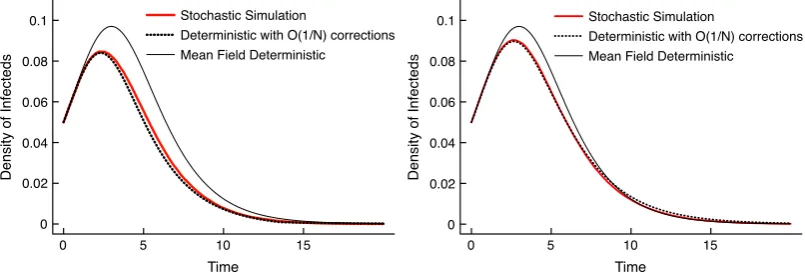
An important feature of stochastic models is the often observed fact that the pre-dicted expected dynamics,E[X] = (E[X](t), t≥0), is not equivalent to solving the
drift part of the decomposition as a related ordinary differential (ODE) problem. That is that for general stochastic differential models,
dX(t) =F(X(t))dt+σ(X(t))dM(t) =6⇒ d
dtE[X(t)] =F(E[X](t)).
to the expected dynamics and an upper bound for the supremum error of this basic approximation.
By taking expectations on equations (2.27) and (2.28) we see that for every disease state indicator process we can make the drift and fluctuation decomposition,
Si(t) =E[Si(t)] + ˜Si(t) (2.29)
Ii(t) =E[Ii(t)] + ˜Ii(t) (2.30)
i= 1, . . . , N.
The time-varying covariance between the random disease indicators, Si(t), Ij(t) is given by the joint expectation of their fluctuations,
cov[Si, Ij](t) =E[ ˜Si(t) ˜Ij(t)] =E[Si(t)Ij(t)]−E[Si(t)]E[Ij(t)].
Whenever cov[Si(t), Ij(t)]6= 0 I say that populations iand j form an SI correlated
pair. I also make the short-hand notation,
cXY(i, j;t) =cY X(j, i;t) = cov[Xi(t), Yj(t)] (2.31)
i, j = 1, . . . , N, X, Y ∈ {S, I, R}, t≥0.
For the SDE representation of the spatial epidemic (2.24), (2.25), the ex-pected dynamics are corrected by the covariance between the susceptibility of each populationiand the infectiousness of each populationj. This can be seen by intro-ducing the drift and fluctuation decomposition to each disease indicator in equations (2.27) and (2.28), taking expectations and applying the martingale property,
d
dtE[Si](t) =−E[Si] X
j(6=i)
K(xi−xj)E[Ij]−
X
j(6=i)
K(xi−xj)cSI(i, j;t)(2.32)
d
dtE[Ii](t) =E[Si] X
j(6=i)
K(xi−xj)E[Ij] +
X
j(6=i)
K(xi−xj)cSI(i, j;t)−γE[Ii],(2.33)
i= 1, . . . , N.
We shall see that the formation of SI correlated pairs is driven by various triple configurations, and can indeed extrapolate that triple configurations are formed by quadruple configurations and so on. This observation plays a key role in so called
closure schemes (Bolker and Pacala 1997) for approximating the statistical
will find that in order to calculate the contribution of SI correlated pairs at any time to the expected dynamics one must first calculate the expected contribution ofSII
and SSI correlated triple configurations. These considerations lead to a hierarchy of correlation dynamics that must be solved. A closure scheme is an approximation of higher order correlations in terms of lower order correlations and the expected dynamics.
The simplest correlation closure is to treat random variables as uncorrelated, i.e. that their covariance is zero. For the spatial epidemic process this is equivalent to the approximation,
E[Si(t)Ij(t)]≈E[Si](t)E[Ij](t), t≥0. (2.34) Applying closure (2.34) to equations (2.32) and (2.33) gives,
d
dtE[Si](t)≈ −E[Si](t) X
j(6=i)
K(xi−xj)E[Ij](t), (2.35)
d
dtE[Ii](t)≈E[Si](t) X
j(6=i)
K(xi−xj)E[Ij](t)−γE[Ij](t), (2.36)
i= 1, . . . , N.
These equations are in ODE form for a closed set of dynamic variables, the expecta-tion processes{E[Si],E[Ii]}Ni=1, and can therefore be solved efficiently using standard
ODE integration techniques such as Runge-Kutta to give an approximation to the expected dynamics that does not require extensive Monte Carlo estimation to solve. However, it is not immediately clear what the size of the error due to using this approximation is, I turn to this question in the next section.
2.3.5 Truncation Error for Pair Covariances
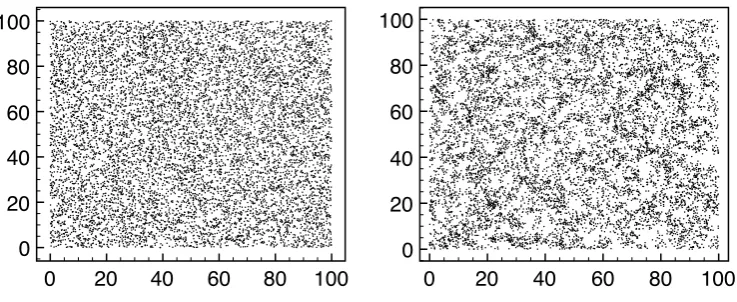
The unfortunate aspect of correlation closure schemes is that the approximation error is generally uncontrolled (see (Murrell, Dieckmann, and Law 2004) for a general discussion on the reliability of closure schemes) and their performance can only be assessed through comparison to Monte Carlo simulation. However, it is clear that the magnitude of the error between the true expected dynamics and the approximations (2.35) and (2.36) is determined by the magnitude of the contribution due to SI

![Figure 2.3: A spatial epidemic on [−10, 10]2 with N = 400. Transmission rate was given bya gaussian shaped kernel, with effort of transmission, K0 = 2, and characteristic length scale oftransmission L = 3](https://thumb-us.123doks.com/thumbv2/123dok_us/9645549.466768/60.595.138.513.192.495/figure-spatial-epidemic-transmission-gaussian-transmission-characteristic-oftransmission.webp)