Almost sharp fronts : limit equations for a two dimensional model with fractional derivatives

University of Warwick institutional repository: http://go.warwick.ac.uk/wrap

A Thesis Submitted for the Degree of PhD at the University of Warwick

http://go.warwick.ac.uk/wrap/55759

This thesis is made available online and is protected by original copyright.

Please scroll down to view the document itself.

Library Declaration and Deposit Agreement

1. STUDENT DETAILS

Please complete the following:

Full  name:  ……….

University  ID  number:  ………

2. THESIS DEPOSIT

2.1 I understand that under my registration at the University, I am required to deposit my thesis with the University in BOTH hard copy and in digital format. The digital version should normally be saved as a single pdf file.

2.2 The hard copy will be housed in the University Library. The digital version will be deposited in the

University’s  Institutional  Repository  (WRAP). Unless otherwise indicated (see 2.3 below) this will be made openly accessible on the Internet and will be supplied to the British Library to be made available online via its Electronic Theses Online Service (EThOS) service.

[At present, theses  submitted  for  a  Master’s  degree  by  Research  (MA,  MSc,  LLM,  MS  or  MMedSci)  are not being deposited in WRAP and not being made available via EthOS. This may change in future.] 2.3 In exceptional circumstances, the Chair of the Board of Graduate Studies may grant permission for an embargo to be placed on public access to the hard copy thesis for a limited period. It is also possible to apply separately for an embargo on the digital version. (Further information is available in the Guide to Examinations for Higher Degrees by Research.)

2.4 If  you  are  depositing  a  thesis  for  a  Master’s  degree  by  Research,  please  complete  section  (a)  below.  

For all other research degrees, please complete both sections (a) and (b) below:

(a) Hard Copy

I hereby deposit a hard copy of my thesis in the University Library to be made publicly available to readers (please delete as appropriate) EITHER immediately OR after an embargo period of

………... months/years as agreed by the Chair of the Board of Graduate Studies. I agree that my thesis may be photocopied. YES / NO (Please delete as appropriate) (b) Digital Copy

I hereby deposit a digital copy of my thesis to be held in WRAP and made available via EThOS. Please choose one of the following options:

EITHER My thesis can be made publicly available online. YES / NO(Please delete as appropriate) OR My thesis can be made publicly available only after…..[date] (Please give date)

YES / NO(Please delete as appropriate) OR My full thesis cannot be made publicly available online but I am submitting a separately identified additional, abridged version that can be made available online.

YES / NO (Please delete as appropriate) OR My thesis cannot be made publicly available online. YES / NO(Please delete as appropriate)

Zoe Catherine Atkins

3. GRANTING OF NON-EXCLUSIVE RIGHTS

Whether I deposit my Work personally or through an assistant or other agent, I agree to the following:

Rights granted to the University of Warwick and the British Library and the user of the thesis through this agreement are non-exclusive. I retain all rights in the thesis in its present version or future versions. I agree that the institutional repository administrators and the British Library or their agents may, without changing content, digitise and migrate the thesis to any medium or format for the purpose of future preservation and accessibility.

4. DECLARATIONS

(a) I DECLARE THAT:

I am the author and owner of the copyright in the thesis and/or I have the authority of the authors and owners of the copyright in the thesis to make this agreement. Reproduction of any part of this thesis for teaching or in academic or other forms of publication is subject to the normal limitations on the use of copyrighted materials and to the proper and full acknowledgement of its source.

The digital version of the thesis I am supplying is the same version as the final, hard-bound copy submitted in completion of my degree, once any minor corrections have been completed.

I have exercised reasonable care to ensure that the thesis is original, and does not to the best of my knowledge break any UK law or other Intellectual Property Right, or contain any confidential material.

I understand that, through the medium of the Internet, files will be available to automated agents, and may be searched and copied by, for example, text mining and plagiarism detection software.

(b) IF I HAVE AGREED (in Section 2 above) TO MAKE MY THESIS PUBLICLY AVAILABLE DIGITALLY, I ALSO DECLARE THAT:

I grant the University of Warwick and the British Library a licence to make available on the Internet the thesis in digitised format through the Institutional Repository and through the British Library via the EThOS service.

If my thesis does include any substantial subsidiary material owned by third-party copyright holders, I have sought and obtained permission to include it in any version of my thesis available in digital format and that this permission encompasses the rights that I have granted to the University of Warwick and to the British Library.

5. LEGAL INFRINGEMENTS

I understand that neither the University of Warwick nor the British Library have any obligation to take legal action on behalf of myself, or other rights holders, in the event of infringement of intellectual property rights, breach of contract or of any other right, in the thesis.

Please sign this agreement and return it to the Graduate School Office when you submit your thesis.

M A

E

G NS

I

T A T

MOLEM

U N

IV_ER

SITAS WARWICEN

SIS

Almost Sharp Fronts : Limit Equations for a

Two-Dimensional Model with Fractional Derivatives

by

Zoe Atkins

Thesis

Submitted to the University of Warwick

for the degree of

Doctor of Philosophy

Mathematics Institute

Contents

List of Figures iii

List of Tables iv

Acknowledgments v

Declarations vi

Abstract vii

Chapter 1 Introduction 1

1.1 An Interpolation Model : The ↵-equation . . . 2

1.2 Motivation . . . 3

1.3 Structure of the Thesis . . . 6

Chapter 2 Preliminary Results 8 2.1 Definition of the Kernel . . . 9

2.2 The Sharp Front Equation . . . 11

2.3 Almost-Sharp Fronts . . . 16

2.4 The Spine of an Almost-Sharp Front . . . 21

2.5 Discussion . . . 27

Chapter 3 Limit Equations in the Smooth Case 29 3.1 Change of Coordinates . . . 30

3.2 Statement of the Theorem . . . 36

3.3 Preliminary Lemmas . . . 38

3.4 The Limit Equation . . . 43

4.2 Derivation of the Limit Equation . . . 59

4.3 Abstract Cauchy-Kovalevskaya Theorem . . . 68

4.4 Existence of Approximate Solutions . . . 69

4.4.1 Function Spaces . . . 70

4.4.2 Existence Theorem . . . 71

4.4.3 Cauchy Estimates . . . 73

Chapter 5 Existence of Exact Solutions to the ↵-equation 78 5.1 Derivation of the Initial Value Problem . . . 79

5.2 Function Spaces . . . 84

5.3 Existence Result . . . 87

5.3.1 Cauchy Estimates on⇠⌦⇠ . . . 88

5.4 Discussion . . . 91

Chapter 6 Analytic Almost-Sharp Fronts 92 6.1 Change of Coordinates . . . 93

6.2 Function Spaces . . . 100

6.3 Initial Value Problem . . . 103

6.3.1 Equations forf andg . . . 104

6.3.2 Equation for ⌦ . . . 106

6.3.3 Cauchy Estimates . . . 108

6.4 Existence Result . . . 109

Chapter 7 Conclusion 111 Appendix A Mathematical Techniques 113 A.1 Convolutions . . . 113

A.2 The Cauchy-Kovalevskaya Theorem . . . 114

Appendix B Smooth Change of Coordinates 116

Appendix C Analytic Change of Coordinates 125

List of Figures

2.1 Sharp Front . . . 12

2.2 Almost - Sharp Front . . . 18

3.1 Change of Coordinates . . . 31

5.1 Bow-Tie Domain -⌃(m0_{) and (m}0_{) . . . . 85}

5.2 Cauchy Estimates . . . 89

6.1 Boundaries of connected regions . . . 93

6.2 R1 . . . 94

6.3 R2 . . . 94

List of Tables

Acknowledgments

Firstly I would like to thank my supervisor Dr. Jose Rodrigo for his help and

ad-vice over the past few years. I am grateful for the time that Jose has set aside, in

addition to the many interesting discussions about open problems for me to work on.

I would also like to thank my parents, sister and Hari for their love, support and

encouragement.

Declarations

I declare that the work contained in this thesis is my own, except where indicated or

cited. This thesis has not been submitted previously for a degree at this or another

Abstract

We consider the evolution of sharp fronts and almost-sharp fronts for the

↵-equation, where for an active scalar q the corresponding velocity is defined by

u = _r?( ) (2 ↵)/2_{q for 0 < ↵ < 1. This system is introduced as a model}

interpolating between the two-dimensional Euler equation (↵ = 0) and the surface

quasi-geostrophic (SQG) equation (↵ = 1).

The study of such fronts for the SQG equation was introduced as a natural

extension when searching for potential singularities for the three-dimensional Euler

equation due to similarities between these two systems, with sharp-fronts

corre-sponding to vortex-lines in the Euler case (Constantin et al., 1994b).

Almost-sharp fronts were introduced in C´ordoba et al. (2004) as a

regulari-sation of a sharp front with thickness , with interest in the study of such solutions

as _! 0, in particular those that maintain their structure up to a time

indepen-dent of . The construction of almost-sharp front solutions to the SQG equation is

the subject of current work (Fe↵erman and Rodrigo, 2012). The existence of exact

solutions remains an open problem.

For the ↵-equation we prove analogues of several known theorems for the

SQG equations and extend these to investigate the construction of almost-sharp

front solutions. Using a version of the Abstract Cauchy Kovalevskaya theorem

(Sa-fonov, 1995) we show for fixed 0<↵<1, under analytic assumptions, the existence

and uniqueness of approximate solutions and exact solutions for short-time

inde-pendent of ; such solutions take a form asymptotic to almost-sharp fronts. Finally,

Chapter 1

Introduction

The Navier-Stokes equation for incompressible fluid flows inRn(n= 2 or 3) is given by:

@u

@t +u·ru ⌫ u= rp+f, (1.1)

r·u= 0, (1.2)

where, for positionx2Rn _{and time t 0, the vector valued function u(x, t)2R}n represents the advective fluid velocity,⌫ 0 the kinematic viscosity, and the scalar functionp(x, t) the pressure1_{. In the most general form of these equations as given}

in (1.1), f represents an external forcing term; in this thesis we will study a model that contains no such term. Equation (1.2) is the incompressibility condition. For a derivation of this equation see, for example, Chorin and Marsden (1979).

In this work we will study a system that interpolates between the two-dimensional Euler equation and the surface quasi-geostrophic equation. The Euler equations for incompressible flow (with no external forcing) are obtained by setting

⌫= 0 in (1.1), that is:

1_{The standard gradient operator}

rin spatial coordinates gives the following:

(u·ru)i= n X

j=1

uj @ui @xj

,

r·u=

n X

i=1

@ui @xi

,

and the Laplace operator in the spatial variables is defined by =Pn

i=1

@2

@x2

i

@u

@t +u·ru= rp, (1.3)

r·u= 0. (1.4)

The surface quasi-geostrophic (SQG) equation - a two-dimensional evolution equation for an active scalarq - is given by:

Dq

Dt =@tq+u·rq = 0, (1.5)

where the velocity uis defined in terms of a stream function :

u= (u1, u2) =r? ⌘

✓

@ @y,

@ @x

◆

, (1.6)

( )1/2 _{=q, (1.7)}

so that:

u=r?( ) 1/2

q. (1.8)

Forx₂R2 _{andt 0, the scalar functionq(x, y, t) represents the potential}

tempera-ture andu, as above, is the fluid velocity. For more information on stream functions see Acheson (1990). In particular, the incompressibility condition is automatically satisfied.

The SQG system is derived from more general equations modelling nonho-mogeneous fluid flow in a rapidly rotating two-dimensional boundary of the three-dimensional half-space, with small Rossby and Ekman numbers (accounting for the rotation and dissipation), and with constant potential vorticity. For a detailed derivation of this system see Pedlosky (1987), and for an overview of the main steps required see Majda and Tabak (1996).

1.1

An Interpolation Model : The

↵

-equation

The focus of this thesis is the study of sharp fronts and almost-sharp fronts for the

Dq

Dt =@tq+u·rq = 0, (1.9)

where q(x, y, t) is a scalar function and the associated velocity u(x, y, t) is defined in terms of a stream function (x, y, t):

u= (u1, u2) =r? ⌘

✓

@ @y,

@ @x

◆

, (1.10)

where:

( )(2 ↵)/2

=q, (1.11)

so that we recover:

u=_r?( ) (2 ↵)/2_{q. (1.12)}

We user? _{to denote the perpendicular gradient operator,r}?_{= ( @}

y,@x), and by the definition of the velocity given in (1.10), u automatically satisfies the incom-pressibility condition_r·u= 0.

We consider this system posed on the two-dimensional cylinder, that is (x, y)_2R/⇡_Z⇥R, for time t₂[0, T]. We focus only on the cases where 0<↵<1; when↵ = 1 we recover the two-dimensional surface quasi-geostrophic (SQG) equa-tion, and for↵= 0 the two-dimensional Euler equation. The↵-equation (1.9)-(1.12) represents an interpolation between these two extremes (C´ordoba, Fonelos, Mancho and Rodrigo, 2005).

On the cylindrical domain, the stream function is given by, on inversion of (1.11), the convolution of q with a kernel of the operator ( ) (2 ↵)_/2_{. We}

introduce two forms of this kernel, alongside Riesz operators, in the next chapter; for more details see C´ordoba, Fe↵erman and Rodrigo (2004).

1.2

Motivation

(C´ordoba et al., 2005). At present the existence of finite time singularities in this case also remains an open question.

The interest in studying potential singularity formation for the SQG equation are its connections to three-dimensional Euler. The SQG equation is presented as a two-dimensional system that is much simpler to study, yet retains many of the features of Euler. The main similarity between the two systems is the structure of the evolution for _r?✓ and the vorticity stream formulation for three-dimensional Euler, where the vorticity!=r ⇥u:

D_r?✓

Dt = (ru)r

?_{✓ and} D!

Dt = (ru)!

respectively. This leads to several analogies between the two systems relating to the characterization of potential singular solutions, construction of the velocity and conserved quantities. Such comparisons are well documented in the literature, see for example Constantin, Majda and Tabak (1994a), Constantin, Majda and Tabak (1994b), Majda and Bertozzi (2002) and Rodrigo Diez (2004).

For the SQG equations, the search for singular solutions has been focused on sharp fronts - weak solutions that attain two constant values in two regions separated by a smooth curve'(Rodrigo, 2004). The physical motivation for study of these solutions is the formation and evolution of weather fronts, discontinuities between masses of hot and cold air (C´ordoba et al., 2004). Numerical evidence for the development of sharp fronts which become singular in finite time has been given in both Constantin et al. (1994a) and Constantin et al. (1994b). The interest in these particular solutions of the SQG equations is that they are analogous to the study of vortex lines for the three-dimensional Euler equation. A derivation of the sharp-front equation is contained in Rodrigo Diez (2004). This is a contour dynamics equation (CDE) describing the evolution of the smooth curve ', and it was shown that smooth solutions to such a CDE exist in short time using a Nash-Moser type argument.

of the sharp front, with a -neighbourhood around'in which the solution changes from one constant to another. In C´ordoba et al. (2004) it is shown that the evolution of the almost-sharp front behaves as the sharp-front equation (CDE) up to some error O( log ), and in Fe↵erman, Luli and Rodrigo (2012) a curve, the spine, is introduced that satisfies the CDE up to an error O( log ). These results rely on the existence of almost-sharp fronts.

Current study is now focused on the construction of these almost-sharp fronts for the SQG equation and their behaviour in the limit as the thickness of the front approaches 0. Of most interest are almost-sharp fronts that maintain their structure up to a time independent of (Fe↵erman et al., 2012). Here, the authors construct a family of almost-sharp fronts indexed by the thickness of the front , and derive an equation for the evolution of such a solution in the limit. It remains an open question as to whether smooth solutions to this equation exist due to the appear-ance of a Prandtl-like term; see for example Sammartino and Caflisch (1998a) and Sammartino and Caflisch (1998b).

A natural system to study in search of singularities is the ↵-equation as described in (1.9)-(1.12) and introduced in C´ordoba et al. (2005). In this paper numerical evidence is outlined showing that sharp fronts for this equation develop singularities when 0 < ↵ _ 1, and a local existence result is given for the corre-sponding CDE. When↵<1 the equation becomes simpler to study as the velocity is less singular than in the SQG case; in particular there is no logarithmic behaviour. In this thesis we construct solutions to the↵-equation; these will either be of a form asymptotic to almost-sharp fronts, and in the final case will be almost-sharp fronts. We prove a series of existence and uniqueness results for such solutions under analytic assumptions, using a version of the Abstract Cauchy Kovalevskaya (ACK) theorem (Safonov, 1995), for 0<↵<1; these results are all new and remain open for the SQG case. Of particular interest is whether we can show existence of almost-sharp front solutions to the ↵-equation and recover almost-sharp front solutions to the SQG equations in the limit as↵_!1.

We derive limit equations for almost sharp front solutions in the smooth case as seen for the SQG equations in Fe↵erman and Rodrigo (2012). For this case we discuss the existence of approximate solutions to the↵-equation; although we obtain a simpler form of the limit equation when 0< ↵ < 1, at present the existence of solutions remains an open problem due to the presence of a Prandtl-like term.

are able to prove existence, and the uniqueness of approximate solutions (which are aymptotic to almost-sharp fronts) to the↵-equation. We extend this result to show that we actually have exact solutions of the same form for some time independent of . The methods for proving existence in these cases have been introduced with the hope to extend these results to the↵= 1 case; we outline several problems with this following the presentation of these results.

The final result obtained in the thesis expands on this idea by the intro-duction of a second method for studying solutions to the ↵-equation. We show that we do indeed have existence of almost-sharp front solutions to the↵-equation that maintain their structure in short-time independent of . This remains an open question for the SQG case.

1.3

Structure of the Thesis

The thesis is e↵ectively broken into two parts; the first half of the thesis (Chapters 2, 3 and the first part of Chapter 4) contain analogues of results that have been shown for the SQG equations, presented in Rodrigo (2004), C´ordoba et al. (2004), Fe↵erman et al. (2012), Fe↵erman and Rodrigo (2012) and Fe↵erman and Rodrigo (2011a), for the case when 0< ↵ <1, and a discussion of the di↵erences between the two systems. The second part of the thesis contains a series of existence results, to be outlined below, for analytic solutions to the ↵-equation, which remain open problems for the SQG case.

The main mathematical tools utilised throughout the thesis are properties of the convolution of two functions and the ACK theorem. An overview of these techniques, including a comparison of the standard Cauchy-Kovalevskaya theorem to the ACK theorem, are contained in Appendix A.

et al. (2004), and Fe↵erman et al. (2012).

In Chapter 3, we construct a family of smooth almost-sharp fronts⌦indexed by the width of the front . For this specific family we find the associated limit equation; under the assumptions that ' satisfies the SFE and that ⌦ has Sobolev bounds independent of , we are able to take the formal limit as !0. A discussion on the validity of these assumptions is contained in§3.1. Existence of solutions to the limit equation in the smooth case, which would be approximate solutions to the ↵-equation, is not yet known. This result is a analogue of that for the SQG equations as presented in Fe↵erman and Rodrigo (2012). We are however able to obtain such an existence results under analytic assumptions.

Chapter 4 contains the analogous result under the assumptions of analytic-ity. We first construct a family of solutions that are asymptotic to almost sharp fronts and, under a suitable change of coordinates derive the corresponding limiting equation obtained by taking the formal limit as !0 (again assuming that the SFE is satisfied). The ACK theorem which is used in the existence results that follow is outlined in §4.3. Associating an IVP with the limit equation we are able to show, using the ACK theorem, that there exists a unique solution, in short time, to the limit equation which takes the form of an approximate almost-sharp front.

Of interest however are exact solutions to the ↵-equation whose time of existence is independent of the width of the front . This forms the remainder of the thesis.

Under the assumpitions of analyticity, in chapter 5 we prove the existence of a family of exact solutions to the ↵-equation; these will be of the same form introduced in Chapter 4. Applying the ACK theorem for function spaces defined within this chapter gives the existence and uniqueness result required. In addition we are also able to ensure that the existence holds for short-time independent of . Chapter 6 contains a new method for constructing analytic almost-sharp front solutions to the ↵ equation. Rewriting the ↵-equation under a new change of variables, a final application of the ACK theorem ensures the existence of such solutions in short-time, again independent of .

Chapter 2

Preliminary Results

In this chapter we present several results for particular solutions of the↵-equation, namely those of sharp fronts and almost-sharp fronts, which will be introduced formally in§2.2 and§2.3 respectively. The theorems contained here are all analogues of existing results for the SQG equations (that is when ↵ = 1) as introduced in Rodrigo (2004), Rodrigo Diez (2004), C´ordoba et al. (2004) and Fe↵erman et al. (2012).

Recall that we are considering the following system:

Dq

Dt =@tq+u·rq = 0, (2.1)

whereu is given by:

u=r?( ) (2 ↵)/2_{q, (2.2)}

posed on the two-dimensional cylinder (x, y) _{2 R}/⇡_Z⇥R, for time t ₂[0, T]. We have periodic behaviour in thex-variable, and so any functions on this domain will be defined for (x, y) 2 [ ⇡₂,⇡₂]⇥R and extended periodically to the whole plane. We restrict our attention to the case when 0<↵ <1, as detailed previously.

The velocity u can be written as the convolution with some kernel K such that u =K⇤q, where K is to be defined. The main di↵erences that occur in the proofs that follow - when compared to those for the SQG equations - are due to di↵erences in the structure of the kernel of the fractional Laplacian for di↵erent exponents, specifically the change in the singular behaviour of these at the origin as

↵_!1. A summary of the form of the kernels that we will employ throughout this thesis, and their corresponding behaviour, is discussed in the next section.

curve ', and derive a contour dynamics equation for the evolution of this curve -the “sharp front equation” - important for studying -the limit equations in Chapters 3 and 4. In§2.3 we introduce a family of almost-sharp fronts, which are a regulari-sation of the sharp fronts, and show that the evolution equation for'is the same as that of the sharp front up to some error term, with size to be determined based on the thickness of the front. An improvement on this result is given in§2.4. Following on from Fe↵erman et al. (2012), we define a special curve, the “spine”, and show that this also evolves as the sharp front equation up to some error term, which is much smaller than in the more general case.

2.1

Definition of the Kernel

We first review the inverse fractional Laplacian in the two-dimensional plane indexed by : ( ) for 0< <1. When posed on the whole plane, for a given function

f that is sufficiently smooth, the Reisz potentials as defined in Stein (1970) are as follows:

(I f)(x) = ( ) f(x) = 1 ( )

Z

R2

|x y|2 2f(y)dy, (2.3)

where the constant is given by:

( ) = ⇡2

2 _{( )}

(1 ), (2.4)

and is the Gamma function1. Note that we will make a particular choice of below as required for the↵-equation, that is = 2₂↵.

The form of the fractional Laplacian on the two-dimensional cylindrical do-main can be derived using standard reflection methods, see for example Evans (1998). The kernel for this operator, extending the case from ↵ = 1 in Rodrigo (2004), is given by:

(u, v)

(u2_+v2₎(2 2 )_/2 +⌘(u, v), (2.5)

where (u, v) 2 C₀1, (u, v) = 1 for |u v| r and supp ⇢ {|u v| R} with 0< r < R < 1₂, and⌘(u, v)2C₀1 with⌘(0,0) = 0. In addition, is periodic in the first argument with period⇡.

1_{For >0, ( ) =}1R 0

By commutativity of the di↵erential operators that appear, we rewrite the velocity u (2.2) in the form u = ( ) (2 ↵)/2_{r?q. Posed on the two-dimensional}

cylinder, u can be written as a convolution with a kernel of the form (2.5). For

↵₂(0,1) we have u=K↵⇤ r?q where:

K↵(u, v) =

(u, v)

(u2_+v2₎↵_/2 +⌘(u, v), (2.6)

that is:

u(x, y) = Z

R/Z⇥R

K↵(x x, y¯ y¯)rx,?¯y¯q(¯x,y¯)d¯xd¯y.

Remark 2.1. By the symmetry methods used to derive the form of this kernel K↵ on the cylindrical domain, the smooth function⌘ is not uniquely defined; to simplify some of the calculations, without loss of generality, we set⌘_⌘0.

The above form for the velocity will be used for deriving the limit equation in the smooth case. The study of the limit equations in the analytic case and the subsequent existence results require an equivalent kernel that is analytic in both variables. We will useu= ˜K↵⇤ r?_{q where:}

˜

K↵(u, v) =

1

(cosh(v) cos(u))↵_/2. (2.7)

This kernel is automatically periodic in the first variable with period 2⇡, and has the same singularity type asK↵ at the origin. To see this recall the Taylor expansions

of the cosh and cos functions about the origin, which give:

cosh(v) cosh(u)_⇡ 1 2(u

2_+v2_{) +h.o.t.}

Remark 2.2. Notice that the kernel K↵ (2.6) corresponds to periodising the kernel obtained by inverting the↵-Laplacian inR2 (which is analytic except for a singularity at the origin). The kernelK↵˜ defined in (2.7) is also analytic except for a singularity at the origin (of the same order).

When ↵<1 these kernels are integrable, in particularK↵ 2L1(R/⇡Z⇥R)

(and ˜K↵ 2 L1(R/2⇡Z⇥R)). For consistency, by applying a scaling to the latter

that only alters any constants we are able to define a version of ˜K↵ of period ⇡; in

doing so we are then able to present all results on the domainR/⇡Z_⇥R.

The theorems presented in the remainder of this chapter will be stated and proved only forK↵. The results for the second kernel are analogous.

2.2

The Sharp Front Equation

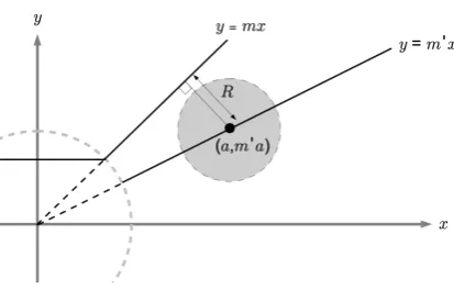
We now focus on sharp fronts for the↵-equation. For the SQG equations the study of sharp fronts is presented as an analogue of the vortex patch problem for the two-dimensional Euler equations (Rodrigo, 2004). For the interpolation model we continue to study the evolution of a particular solution to the system (2.1)-(2.2) that takes constant values in two regions separated by a smooth curve (see Figure 2.1). We derive an equation for the evolution of such a curve.

In Rodrigo Diez (2004), in the study of the SQG equations, two di↵erent derivations for the corresponding “sharp front equation” are presented - the study of the equations in the limit approaching the curve and using weak solutions. Here, for (2.1)-(2.2) we derive the analogous equation using the latter; we assume existence of a weak solution to the↵-equation for short time taking the form of a sharp front, and derive an evolution equation for the given boundary curve. The standard definition of a weak solution to (2.1) is as follows:

Definition 2.3. A bounded function q is a weak solution for the ↵-equation (2.1) if for any ₂C₀1(R/⇡Z_⇥R_⇥[0, T])

ZZZ

[0,T]⇥R⇥R/⇡Z

q(x, y, t)@t (x, y, t) dxdydt

+

ZZZ

[0,T]⇥R⇥R/⇡Z

q(x, y, t)u(x, y, t)_·r (x, y, t) dxdydt= 0, (2.8)

where u is defined in (2.2).

A sharp front is defined to be a solution that satifies two constant values in two regions, which change sharply over a boundary given by a smooth curve

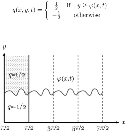
q(x, y, t) = (

1

2 if y '(x, t)

1

2 otherwise

(2.9)

as illustrated.

Figure 2.1: Sharp Front

Remark 2.4. Note that in both Rodrigo Diez (2004) and Rodrigo (2004) the con-stants used for the di↵erent regions are instead 0 and 1. Without loss of generality we choose the values 1₂ and 1₂; for later proofs within the paper this choice pro-vides some cancellation of terms and enables us to simplify the calculations. For consistency we use this definition throughout the thesis. For the proofs that follow in this section, the change of constants only require elementary changes from the SQG case.

We now study the evolution of'(x, t), and derive the following:

Theorem 2.5(Sharp Front Equation 1). Let q be a weak solution of the↵-equation as defined in (2.1), and letq be of the form (2.9). Then the function 'satisfies the equation:

@'

@t(x, t) =

Z

R/⇡Z

@' @x(x, t)

@' @x¯(¯x, t)

[(x x¯)2_{+ ('(x, t) '(¯x, t))}2_]↵_/2 (x x,¯ '(x, t) '(¯x, t))d¯x

+ Z

R/⇡Z

✓

@' @x(x, t)

@' @x¯(¯x, t)

◆

where, for consistency with existing work, the notation @_@f_x¯(¯x, t) = @_@f_x(¯x, t) is used to denote di↵erentiation with respect to the spatial variable.

When considering the analytic case, as presented in Remark 2.2, we use an equivalent kernel. The same set of calculations gives a similar statement when we consider the kernel ˜K↵ (2.7):

Theorem 2.6(Sharp Front Equation 2). Let q be a weak solution of the↵-equation as defined in (2.1), and letq be of the form (2.9). Then the function 'satisfies the equation:

@'

@t(x, t) =

Z

R/⇡Z

@' @x(x, t)

@' @x¯(¯x, t)

(cosh('(x, t) '(¯x, t)) cos(x x¯))↵_/2d¯x. (2.11)

Both forms of the sharp front equation will be utilised when deriving the limit equations in Chapters 3 and 4.

The proof of Theorem 2.5, up to the choice of constants, remains the same as that presented in Rodrigo (2004). For completeness and in order to introduce some of the notation, we give an overview of the details here. The methods used in Rodrigo (2004) for the SQG equations in e↵ect show that if we have a system as in (2.1) with the function u of the formu =r?_{K ⇤q for some kernel K, then} assuming thatK is regular enough that all integrals make sense, the proof can be generalised further.

Proof of Theorem 2.5. Note that for all ↵ < 1 it follows from the definition that

r?K↵2L1. Givenu=r?K↵⇤q, sinceq2L1an application of Young’s inequality

for convolutions (Theorem A.1) gives u 2 L1 and so all of the integrals below are well defined. We first set:

I ={(x, y, t) :y '(x, t)}, II={(x, y, t) :y <'(x, t)},

whereq_⌘ 1₂ on I andq _⌘ 1₂ on II. The outward unit normals for each region, as required for integration by parts, are respectively:

⌫I(x, y, t) = (⌫_xI,⌫_yI,⌫_tI) = (@x', 1,@t') (1 + (@x')2+ (@t')2)1/2

,

⌫II(x, y, t) = (⌫_xII,⌫_yII,⌫_tII) = ( @x',1, @t') (1 + (@x')2+ (@t')2)1/2

.

the weak solution (2.8) and derive an equation for the evolution of the curve '. Evaluating the first term in this definition, an integration by parts gives:

ZZZ

[0,T]⇥R⇥R/⇡Z

q@t dxdydt= ZZZ

y '(x,t)

1

2@t dxdydt

ZZZ

y<'(x,t)

1

2@t dxdydt

= 1

2 ZZ

y='(x,t)

⌫_tI(1 + (@x')2+ (@t')2)dxdt 1 2

ZZ

y='(x,t)

⌫_tII(1 + (@x')2+ (@t')2)dxdt

= 1

2 ZZ

y='(x,t)

@t'dxdt 1 2

ZZ

y='(x,t)

( @t')dxdt

= ZZ

y='(x,t)

@t'dxdt. (2.12)

Considering only the spatial integration to begin with, we study the second term in (2.8). Introducing limits and on integrating by parts we obtain:

ZZ

R⇥R/⇡Z

qu·r dxdy= 1 2 lim!0

Z

y='(x,t)+

u · @x'

1 !

dx

1 2 lim!0

Z

y='(x,t)

u · @x'

1 !

dx, (2.13)

where:

u · @x'

1 !

= 1

2 (x, y, t) Z

¯

y '(¯x,t)

r?x,yK↵(x x, y¯ y¯)·

@x' 1

! d¯xd¯y

1

2 (x, y, t) Z

¯

y<'(¯x,t)

r?x,yK↵(x x, y¯ y¯)·

@x' 1

! d¯xd¯y

=A1+A2.

A1=

1

2 (x, y, t) Z

¯

y '(¯x,t)

r?x,¯y¯K↵(x x, y¯ y¯)·

@x' 1

! d¯xd¯y

= 1

2 (x, y, t) Z

¯

y '(¯x,t)

r¯x,y¯K↵(x x, y¯ y¯)·

1

@x' !

d¯xd¯y

= 1

2 (x, y, t) Z

¯

y '(¯x,t)

r¯x,y¯·

K↵(x x, y¯ y¯) @x'K↵(x x, y¯ y¯)

! d¯xd¯y

= 1

2 (x, y, t) Z

¯

y='(¯x,t)

K↵(x x, y¯ y¯) 1

@x' !

· @x¯'

1 !

d¯x

= 1

2 (x, y, t) Z

¯

y='(¯x,t)

K↵(x x, y¯ y¯) (@x¯' @x') d¯x

and similarly forA2. This gives:

u _· @x'

1 !

= (x, y, t) Z

¯

y='(¯x,t)

✓

@' @x¯

@' @x

◆

K↵(x x, y¯ y¯)d¯x, (2.14)

and taking limits as !0 in (2.13) we have:

ZZ

R⇥R/⇡Z

qu·r dxdy= Z

y='(x,t)

(x, y, t) Z

¯

y='(¯x,t)

✓

@' @x¯

@' @x

◆

K↵(x x, y¯ y¯)d¯xdx.

Combining this with (2.12) gives:

ZZ

y='(x,t)

@t'dxdt

+ Z

y='(x,t)

(x, y, t) Z

¯

y='(¯x,t)

✓

@' @x¯

@' @x

◆

K↵(x x, y¯ y¯)d¯xdxdt= 0

@t'= Z

R/⇡Z

✓

@' @x

@' @x¯

◆

K↵(x x, y¯ '(¯x, t))d¯x,

which is precisely the sharp front equation. ⇤

Given an initial condition '(x,0) ='0(x) we can consider an initial value

problem for the equation (2.10). For the SQG equations (↵= 1), it has been shown that for smooth, periodic functions '0 the system had a unique smooth solution

for a small time. This has been proved in Rodrigo Diez (2004) using a Nash-Moser argument. For other values of↵, local existence and uniqueness of smooth solutions to the corresponding IVP has been outlined in C´ordoba et al. (2005) using the same argument. In Fe↵erman and Rodrigo (2011b) the authors show that, on application of a version of the Abstract Cauchy-Kovalevskaya theorem that given an IVP for the sharp-front equation with analytic initial data, there exists a unique analytic solution in short-time.

For 0 < ↵ < 1 Gancedo (2008) defines a more general almost sharp front, that is:

q(x1, x2, t) =

(

q1 ⌦(t)

q2 R2/⌦(t)

whereq1andq2are constant and the boundary is parametrised by@⌦(t) ={x( , t) =

(x1( , t), x2( , t)) : 2[ ⇡,⇡]}. An equivalent CDE to (2.10) and (2.11) is derived

and the author shows that, under additional assumptions on the boundary2, for

x0( )2Hk(T) where k 3, then there exists a timeT >0 such that there exists a

unique solution to the associated IVP inC1([0, T];Hk(T)).

2.3

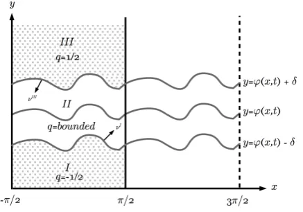
Almost-Sharp Fronts

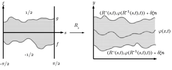
We now turn our attention to the evolution of almost-sharp fronts for the↵-equation (2.1)-(2.2). These are a regularisation of sharp fronts as introduced previously, and are weak solutions of the ↵-equation (see Definition 2.3) that take two constant values which change in a transition strip of width 2 ; these solutions have large gradient of order 1. The transition layer is defined as a -neighbourhood of a given

2_{For F(x) =:} |⌘|

|x( ,t) x( ⌘,t)| 8 ,⌘ 2 [ ⇡,⇡] and F(x)( ,0, t) = |@ x1( ,t)| it is required that

smooth curvey='(x, t). We remain in the cylindrical case and define almost-sharp fronts to be weak solutions of the form:

q(x, y, t) = 8 > < > :

1

2 if y '(x, t) +

bounded if |'(x, t) y|

1

2 if y'(x, t)

(2.15)

where'is periodic inx; these are illustrated in Figure 2.2.

In this form we derive an evolution equation for the curve'(x, t); we show that this curve in fact satisfies the sharp front equation (Theorems 2.5 and 2.6) up to some error term of order (the same error for which the function 'is defined in (2.15)).

This problem was introduced in C´ordoba et al. (2004) for the SQG equations,

↵= 1, and the authors show that the curve'satisfies the corresponding sharp-front equation up to some error of size log . The following result shows that when↵<1 we obtain a better estimate due to the singularity of the kernel in this case.

Theorem 2.7. Let q be a weak solution of the ↵-equation (2.8), and let q be of the form (2.15), then the curve' satisfies the following equation:

@'

@t(x, t) =

Z

R/⇡Z

@' @x(x, t)

@' @u(u, t)

[(x u)2_{+ ('(x, t) '(u, t))}2_]↵_/2 (x u,'(x, t) '(u, t))du

+ Z

R/⇡Z

✓

@' @x(x, t)

@' @u(u, t)

◆

⌘(x u,'(x, t) '(u, t))du+Error,

where _|Error_|C withC depending only on _kq_k1 and_kr'_k1.

We introduce the notation X = O(Y) when _|X_{| } C_|Y_|, where in the fol-lowing the constant C will depend only on kqkL1, kr'k_L1 and k k_C1 which are

independent of . Note that we use the standard norms in each of these function spaces, for details see Evans (1998).

Figure 2.2: Almost - Sharp Front

Proof of Theorem 2.7. We first define the three regions as introduced in (2.15); these are illustrated in Figure 2.2. Let:

I =_{(x, y) :y_'(x, t) _}, II =_{(x, y) :_|y '(x, t)_|< _}, III =_{(x, y) :y '(x, t) + _},

with the corresponding outward unit normals for regionsI and III as follows:

⌫I(x, y, t) = (⌫_xI,⌫_yI,⌫_tI) = ( @x',1, @t') [1 + (@x')2+ (@t')2]1/2

,

⌫III(x, y, t) = (⌫_xIII,⌫_yIII,⌫_tIII) = (@x', 1,@t') [1 + (@x')2+ (@t')2]1/2

.

In order to simplify the calculations in the arguments that follow, we prove this theorem for the almost-sharp front defined as in C´ordoba et al. (2004):

q(x, y, t) = 8 > < > :

1 if y '(x, t) +

bounded if _|'(x, t) y_|

0 if y'(x, t)

(2.16)

We substitute this definition into that of the weak solutions (2.8). The same esti-mate, presented in Theorem 2.7, holds for the previous definition (2.15), which we employ throughout the thesis.

defined in (2.16). To see that the proof also holds for the previous definition (2.15), letq˜be an almost sharp front of the form in (2.15). Then forq as in (2.16) we have

˜

q=q+1₂. We note that the corresponding velocities are the same, that is:

u=K⇤ r?q=K⇤ r?(q+1

2) =K⇤ r ?_q,˜

and so all integral estimates presented within the proof of this theorem hold for the almost-sharp front in (2.15).

Note that:

ZZZ

I⇥[0,T]

q(x, y, t)@t (x, y, t)dxdydt+ ZZZ

I⇥[0,T]

q(x, y, t)u(x, y, t)_·r (x, y, t)dxdydt= 0

and so we study in detail the contributions from the other two regions.

We first show that the integrals over regionII contribute to the error terms, that is they areO( ). Note that the area of this region isO( ) with dependence on

kr'_kL1. We have:

ZZZ

II⇥[0,T]

q(x, y, t)@t (x, y, t)dxdydt kqkL1k k_C1.

Foru=_r?K↵⇤q withr?K↵ 2L1 andq bounded, it follows, by an application of

Young’s inequality for convolutions, that_ku_k1C_kq_k1 giving: ZZZ

II⇥[0,T]

q(x, y, t)u(x, y, t)_·r (x, y, t)dxdydt_{ k}q_k2_L1k kC1.

In order to calculate the integrals from regionIII, we introduce a decompo-sition foru;u=uII+uIII =r?K↵⇤q II+r?K↵⇤ III. Note thatuII and uIII are divergence free. Then:

ZZZ

III⇥[0,T]

q(x, y, t)uII(x, y, t)·r (x, y, t)dxdydt kqk2L1k kC1

ZZZ

III⇥[0,T]

q(x, y, t)@t (x, y, t)dxdydt+ ZZZ

III⇥[0,T]

q(x, y, t)uIII(x, y, t)·r (x, y, t)dxdydt.

The former can be calculated using integration by parts as in the proof of Theorem 2.5. That is:

ZZZ

III⇥[0,T]

q(x, y, t)@t (x, y, t)dxdydt= ZZZ

y '(x,t)+

@t (x, y, t)dxdydt

= ZZ

y='(x,t)+

(x, y, t)@t'dxdt,

and for the latter, withuIII divergence free, considering spatial integration only to begin with:

ZZ

III

uIII ·r dxdy= lim

✏!0+

ZZ

y '(x,t)+ +✏

uIII·r dxdy

= lim

✏!0+

Z

y='(x,t)+ +✏

uIII (x, y, t)·

@x' 1

! dx,

where as in§2.2:

uIII (x, y, t)·

@x' 1

!

= (x, y, t) Z

¯

y='(¯x,t)+

K↵(x x, y¯ y¯) (@x¯' @x') d¯x.

Taking limits as✏_!0 and combining the results : ZZ

y='(x,t)+

(x, y, t)@t'dxdt

+ Z

y='(x,t)+

(x, y, t) Z

¯

y='(¯x,t)+

K↵(x x, y¯ y¯) (@x¯' @x') d¯xdxdt

+O( ) = 0

@t'(x, t) = Z

R/⇡Z

K↵(x x,¯ '(x, t) '(¯x, t)) (@x¯' @x') d¯x

as required. In order to adapt the proof for the almost-sharp front defined in (2.15) we use the same techniques alongside the continuity of the integrands and the cor-responding decomposition u = uI +uII +uIII = 1₂r?K↵⇤ I +r?K↵⇤q II +

1

2r?K↵⇤ III. ⇤

2.4

The Spine of an Almost-Sharp Front

In Fe↵erman et al. (2012), given a solution of the SQG equation (↵ = 1) that is locally constant outside a -neighbourhood of a given curve ' that evolves with time, the authors define the concept of the ‘spine’. They show that given an almost-sharp front weak solution of the SQG equation, there exists an associated curve (the ‘spine’) that can be explicitly defined and evolves as the sharp front equation up to some error of size 2_{|log |. This improves the result of C´ordoba et al. (2004)}

as the spine is shown to evolve up to an error smaller than as was previously given (see§2.3). The spine is defined in the transition layer |'(x, t) y|< and is constructed using an argument that estimates the di↵erence between two measures; a delta function on the curve being constructed,µ, andr?_{qdxdy. The construction} is independent of the form of u and so we may extend the definition to the case 0<↵<1; we refer the reader to Fe↵erman et al. (2012) for the details.

In this section we give an analogous result for the ↵-equation for values of 0<↵<1. We show that the associated spine for this equation evolves as the sharp front equation (2.10) up to an error of order 2, giving an improvement on the result presented in§2.3. We first give the definition of the spine and an extended definition of almost sharp fronts as required for the proof.

Definition 2.10. For a function q of the form (2.15) we define the spine (in the region_|'(x, t) y_|< ),y=µ(x), by

Z

R

qy(x, y)(y µ(x))dy= 0 8x. (2.17)

Z

R

qy(x, y, t)(y µ(x, t))dy= 0 8x. (2.18)

Assume thatq is of the form

q(x, y) = 8 > < > :

1

2 if y µ(x) +

smooth if _|µ(x) y_|<

1

2 if yµ(x)

(2.19)

and that it satisfies the growth conditions

|@_xq_|c | | _{8| |}2. (2.20)

A functionq with these properties above will be called an almost-sharp front.

Remark 2.12. The spine condition (2.17) also gives the property:

'(x,t_Z )+

'(x,t)

q(x, y, t)dy = 0 (2.21)

using integration by parts and shown in Fe↵erman et al. (2012).

This definition of an almost-sharp front requires more regularity plus ad-ditional growth conditions than as defined in §2.3. The growth conditions were introduced in Fe↵erman et al. (2012) for construction of the spine. Note that this is the only section in which we use this definition; for the remaining chapters an almost-sharp front will be as defined in§2.3. We prove the following:

Theorem 2.13. Let q be an almost-sharp front for the ↵-equation as in definition 2.11 and letµ be its corresponding spine as introduced in definition 2.10. Then for every test function (x, t), the spine satisfies:

ZZ

R⇥R/⇡Z

(x, t) 

@µ @t(x, t)

Z

R/⇡Z

K↵(x u, µ(x, t) µ(u, t))

✓

@µ @x(x, t)

@µ @u(u, t)

◆

du dxdt

=Error, (2.22)

We will utilise the following result from Fe↵erman et al. (2012):

Corollary 2.14. For µ(x, t) as defined in Definition 2.11, then for every (x, y)

with_|r2 _|M:

ZZ

R/⇡Z⇥R

(x, y, t)_r?q(x, y, t)dxdy= Z

y=µ(x)

(x, y)(1,@µ

@x(x, t))dx+O(M

2_).

Proof of Theorem 2.13 The sharp front equation (2.10) is given by:

µt(x, t) = Z

R/⇡Z



@µ @x(x, t)

@µ

@x¯(u, t) K↵(x u, µ(x, t) µ(u, t))du (2.23)

and given a weak solutionqof the↵-equation with a test function (x, y, t) we have:

ZZZ

[0,T]⇥R⇥R/⇡Z

q(x, y, t)@t (x, y, t)dxdydt (2.24)

+

ZZZ

[0,T]⇥R⇥R/⇡Z

q(x, y, t)u(x, y, t)_·r (x, y, t)dxdydt= 0. (2.25)

We aim to show (2.22) with error O( 2_{). As remarked in Fe↵erman and}

Rodrigo (2011b), (2.22) contains only test functions that depend on x and t: we can assume that this is the case near to the spine. So while (2.24) and (2.25) are true for general test functions (x, y, t) we only need to consider functions that are constant iny near to the curve µ. This family of test functions will suffice to prove the result in (2.22). We sketch only an outline of the proof here and refer to the details in Fe↵erman et al. (2012).

Firstly the term (2.24), by the same method in that paper, is precisely:

ZZ

R/⇡Z⇥R

(x, t)µt(x, t)dxdt+O( 2) (2.26)

using (2.21). This is independent of the kernel chosen.

show that (2.25) is equal to:

ZZ

R/⇡Z⇥R

(x, t) Z

R/⇡Z



@µ @x(x, t)

@µ

@x¯(¯x, t) K↵(x x, µ¯ (x, t) µ(¯x, t))d¯x + O(

2_).

(2.27) Analogously to the proof of Theorem 2.3, we write (2.25) as a sum of integrals taken over the three domainsI,IIandIII. Using the same notation as in Fe↵erman et al. (2012) we consider only the spatial integration of this term and study, using

u=_r?K↵⇤q, the following function B(t). Introducing the notation x= (x, y) ⌘

(x1, x2) and u= (u1, u2) in order to simplify the following, we define:

B(t) = ZZ

x,u2I[III

r?xK↵(x u)q(u)rx (x)q(x)dxdu

+

ZZ

x2I[III,u2II or u2I[III,x2II

r?xK↵(x u)q(u)rx (x)q(x)dxdu

+ ZZ

x,u2II

r?xK↵(x u)q(u)rx (x)q(x)dxdu

=Bouter+Bcross+Binner. (2.28)

The authors show, using integration by parts and symmetrizing some of the integrals, that this is equivalent to studying just three terms:

ZZ

x2I[III,u2II

[_rx (x) ru (u)]r?xK↵(x u)q(x)q(u)dxdu, (B1)

ZZ

x,u2II

K↵(x u)[rx (x) ru (u)]q(u)r?xq(x)dxdu, (B2)

ZZ

x,u2I[III

r?xK↵(x u)q(u)rx (x)q(x)dxdu, (B3)

Z

x2=µ(x1)

Z

u2=µ(u1)

(x1, x2)

✓

@µ @u1

(u1, t)

@µ @x1

(x1, t)

◆

K↵(x u)dx1du1+O( 2),

(2.29) which are precisely the estimates needed to show (2.22).

On integrating by parts, using_r?q = 0 inI_[III, we have:

(B1) = Z

u2II  X

=±1

Z

x2=µ(x1)+

q(u)[_rx (x) ru (u)]K↵(x u)

✓ 1, @µ

@x1

◆

dx1 du

=: Z

u2II

q(u)G(u1, u2)du1du2

= Z

u2II

q(u)[G(u1, u2) G(u1, µ(u1))]du1du2, (2.30)

where (2.30) follows from Remark 2.12. Noting that byK↵ 2L1:

|G(u1, u2) G(u1, µ(u1))|C

for some constantC independent of , and that the domain isO( ), this gives (B1) isO( 2) as required. Next we define:

Q(x) = Z

u2II

K↵(x u)[rx (x) ru (u)]q(u)du (2.31)

and write:

(B2) = Z

x2II

Q(x)r?xq(x)dx. (2.32)

UsingK↵ 2L1 we can show that r2x0Q is bounded. By an application of Corollary

(B2) =O( 2) Z

x2=µ(x1)

Q(x) ✓

1, @µ @x1

(x1, t)

◆ dx1

O( 2) Z

x2=µ(x1)

Z

u2II

K↵(x u)[rx (x) ru (u)]q(u)

✓ 1, @µ

@x1

(x1, t)

◆ dudx1

=O( 2) Z

u2II

q(u) Z

x2=µ(x1)

K↵(x u)[rx (x) ru (u)]

✓ 1, @µ

@x1

(x1, t)

◆ dx1du

(2.33)

=O( 2) + Z

u2II

q(u)P(u)du, (2.34)

whereP(u) is defined by the inner integral in (2.33). Writing:

(2.34) =O( 2) + Z

u2II

q(u)[P(u1, µ(u1)) P(u1, u2)]du (2.35)

using the spine condition in Remark 2.12. Using the same argument as for (B1) on the integral term in (2.35), we obtain that (B2) is preciselyO( 2) as required. For the final term:

(B3) = 1 4

X

1, 2=±1

Z

x2=µ(x1)+ 1

Z

u2=µ(u1)+ 2

(x1, x2)

✓ @µ @u1 @µ @x1 ◆

K↵(x u)dx1du1.

(2.36)

For 1 = 2:

1 4

X

=±1

Z

x2=µ(x1)+

Z

u2=µ(u1)+

(x1, x2)

✓ @µ @u1 @µ @x1 ◆

K↵(x u)dx1du1

= 1

2 Z

x2=µ(x1)

Z

u2=µ(u1)

(x1, x2)

✓ @µ @u1 @µ @x1 ◆

K↵(x1 u1, µ(x1) µ(u1))dx1du1

+O( 2) (2.37)

1 4

X

=±1

Z

x2=µ(x1)+

Z

u2=µ(u1)

(x1, x2)

✓

@µ @u1

@µ @x1

◆

K↵(x u)dx1du1 =F( ).

(2.38)

Noting thatF( ) =F(0) +O( 2_{) follows on showing F}0_{( )C ; the proof is the} same as in Fe↵erman et al. (2012) up to the change in singularity of the kernel and so we omit the lengthy calculations. Combining the estimates on (B1)-(B3) completes

the proof. ⇤

2.5

Discussion

When studying the evolution of sharp fronts for the SQG equation, the analogous problem for three-dimensional Euler is the evolution of a vortex line (as discussed in the Introduction). The derivation of the sharp front equation uses tools not available for the Euler case. Current study involves the study of almost-sharp fronts and the limiting procedure as the thickness of the front approaches 0 as an insight into this problem (C´ordoba et al., 2004).

Within this Chapter, we have summarised several results that have been proven for the SQG equation, regarding estimates on almost-sharp front solutions in the limit as ! 0. For this case ↵ = 1, the existence of almost-sharp front solutions remains an open question; the most important case being the existence of smooth solutions of such a type. In particular, solutions that exist for time independent of . The construction of such solutions is studied in Fe↵erman and Rodrigo (2012).

We study the analogous problem for the↵-equation; that is we attempt to construct almost-sharp front solutions. In studying almost-sharp fronts for this system, we attempt to introduce several methods which could be applied to the SQG case, with the study of this system being simpler (as previously discussed). The most ideal result would be to show that there exist smooth almost-sharp front solutions to (2.1)-(2.2) and study these in the limit as↵_!1. This would also allow us to utilise the results proved within this chapter and to see which estimates we may recover in the limit. However this also remains an open question (see Chapter 3).

Chapter 3

Limit Equations in the Smooth

Case

The results described in the previous chapter (the estimates in both §2.3 and§2.4) assume the existence of almost-sharp fronts for the ↵-equation; the focus of this chapter is the study of their construction. We define below a family of almost-sharp fronts, indexed by a parameter >0 relating to the thickness of the front (as seen in Chapter 2). For this specific family, we derive the limit equations as approaches 0 for each fixed value of↵ and prove an approximation result for smooth solutions. The study of analytic solutions forms the basis of the next chapter. We consider the case only when 0<↵<1; the approximation result stated in§3.2 is an analogue of the result proved in Fe↵erman and Rodrigo (2012) for the SQG equations (↵= 1).

Recall that the ↵-equation is given by:

@tq+u·rq= 0 (3.1)

where:

u= ( ) (2 ↵)/2

r?q. (3.2)

We continue to study this system when posed on a two-dimensional spatial domain (x, y) _{2 R}/⇡_Z⇥R with t ₂ [0, T], that is we are considering periodic behaviour in the horizontal direction. Any functions will be defined for (x, y) ₂ [ ⇡₂,⇡₂]⇥R and extended periodically to the whole plane.

these are regularisations of a sharp front in which the solution changes smoothly between two constant values1 in a small strip along the boundary. We aim to construct a family of almost-sharp fronts - weak solutions of the↵-equation, of the form:

q(x, y, t) = 8 > < > :

1

2 if y '(x, t) +

bounded if _|y '(x, t)_|<

1

2 if y'(x, t)

(3.3)

where, as previously, the given function'(x, t) is periodic in thexvariable, and >0 acts as a parameter for our family of almost-sharp fronts. During the construction it will be shown that it is necessary for the curve y = '(x, t) to satisfy the sharp front equation (2.10).

3.1

Change of Coordinates

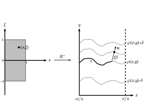
In order to study almost-sharp fronts of the form (3.3), we first need to introduce a smooth change of coordinates, enabling us to study the evolution on a fixed domain of size independent of .

The new coordinates describe a neighbourhood of the curve y = '(x, t) using renormalized arc length, s, and a distance to the curve, ⇠, which will be scaled by the parameter . This coordinate system was introduced in the study of the construction of almost sharp-fronts for the SQG equation (when ↵ = 1), in Fe↵erman and Rodrigo (2012). The change of variables remain the same for the case

↵<1 and this section contains an outline of the required construction as presented in that paper. Appendix B contain full details of the calculations for the results given below.

The renormalised arc length for the curve'(x, t) of period⇡in thex-direction is defined to be:

R(x, t) = 1

L(t) x Z

⇡

2

(1 + ('02(¯x, t)))1/2_{d¯x (3.4)}

where L(t) = R⇡2

⇡

2(1 + ('

02_{(¯x, t)))}1_/2_{d¯x represents the length of the curve. We use}

prime notation to denote the derivative with respect to the first variable. When considered only as a function ofx, R is invertible, and so we use R 1 to construct a map between the fixed domain (s,⇠) ₂ [0,1)_⇥[ 1,1] and the corresponding

-1_{For consistency we continue to choose these values to be} 1 2 and

neighbourhood of the curve'as defined in (3.3), and illustrated in Figure 3.1. This map is given by:

(x, y) = (R 1(s, t),'(R 1(s, t), t)) +n(R 1(s, t))⇠ (3.5)

where n(R 1(s, t)) is the unit normal to the curve ' at the point R 1(s, t), and

t(R 1_{(s, t) the corresponding unit tangent vector:}

n(R 1(s, t)) = ( '0((R

1_{(s, t)), t),1)}

k( '0_((R 1_{(s, t)), t),1)k},

t(R 1(s, t)) = (1,'0((R

1_{(s, t)), t))}

k(1,'0_((R 1_{(s, t)), t))k}.

Figure 3.1: Change of Coordinates

By the definition of the almost-sharp front that was introduced in (3.3), the parameter corresponds to half of the thickness of the front. Since ' is given, it is clear that there exists a value 0, depending on the curvature of ', such that for

 0 the map defined in (3.5) is injective. At this point we also introduce a new

time variable⌧ and now consider, in the new variables, a family of solutions to the

↵-equation of the form:

q(x, y, t) =⌦(s,⇠,⌧) (3.6)

⌦(s,⇠,⌧) = 8 > < > :

1

2 ⇠ 1

smooth |⇠|<1

1

2 ⇠  1

(3.7)

Remark 3.1. For the same reasoning as in Chapter 2, the constant values of ⌦ have been chosen in such a way that we get some cancellations, which simplify the results that follow. In this case we have that R₁1⌦⇠d⇠= 1, and⇠⌦(⇠,⌧)|11 = 0.

The fixed domain as constructed is of size independent of and so the family of solutions defined in (3.7) lose some of their dependence on , and their behaviour is somewhat controlled. In fact, it is clear from the construction that⌦will be smooth in all variables; the derivatives will still depend on which will be seen shortly. In order to study the limit equations we will assume that the Sobolev norms of⌦with respect to the variables s and ⇠, while dependent on , are uniformly bounded for all _ 0. This is not known to be true in the smooth case - in Chapter 6 we obtain

a construction of a family of almost-sharp fronts which satisfy this assumption. In Fe↵erman and Rodrigo (2012) it is remarked that when↵= 1 the dependence of ⌦

on is bad, in such a way that the ⌧-derivative of ⌦ is logarithmic in . We show that for 0<↵<1 the singularities concerned mean that we do not encounter this logarithmic behaviour, and obtain a much simpler form for the limit equation.

We now write the ↵-equation in terms of ⌦(s,⇠,⌧) as defined above, where we have:

(x, y, t) = (R 1(s,⌧),'(R 1(s,⌧),⌧),⌧) + ✓

( '0((R 1(s,⌧)),⌧),1)

k( '0_((R 1_{(s,⌧)),⌧),1)k}⇠ ,0

◆ (3.8)

and simplify some of the terms that appear by writing'(s) ='(R 1_(s,⌧)),'0_{(s) =} '0(R 1(s,⌧)) and'00(s) ='00(R 1(s,⌧)). When it is clear, we will suppress some of the arguments. We first have that:

@x= 1

Det(s)

@y @⇠@s

1

Det(s)

@y

@s@⇠, @y =

1

Det(s)

@x @s@⇠

1

Det(s)

@x @⇠@s,

@t=

I

Det(s)@s+

II

Det(s) = @x @s @y @⇠ @x @⇠ @y

@s, I = @x @⇠ @y @⌧ @x @⌧ @y

@⇠, II = @x @⌧ @y @s @x @s @y @⌧ with: @x @s =R

1

s +



'00R_s1

(1 +'02_(s))1_/2 +

'02'00R_s1

(1 +'02_(s))3_/2 ⇠ ,

@y @s ='

0_R 1

s

'0'00R_s1

(1 +'02_(s))3_/2⇠ ,

@x @⇠ =

'0

(1 +'02_(s))1_/2,

@y

@⇠ = (1 +'02_(s))1_/2,

@x @⌧ =R

1

⌧ +



'00R_⌧1 '0_⌧

(1 +'02_(s))1_/2 +

'02('00R_⌧1+'0_⌧) (1 +'02_(s))3_/2 ⇠ ,

@y @⌧ ='

0_R 1

⌧ +'⌧

'0('00R 1

⌧ +'0⌧)

(1 +'02_(s))3_/2 ⇠ .

Using the inverse function theorem to determine thatR 1

s = _(1+'0L2_(s))1/2, we

find the following simplified terms:

Det(s) =L L '00(s)

(1 +'02_(s))3_/2⇠

2_{, (3.9)}

I =

(1 +'02_(s))1_/2



(1 +'02(s))R_⌧1 '0(s)'⌧(s) + '00(s)R

1

⌧ +'0⌧(s)

(1 +'02_(s))1_/2 ⇠ ,

II = L'⌧(s) (1 +'02_(s))1_/2 +

L'00(s)'⌧(s)

(1 +'02_(s))2⇠ ,

and a series expansion provides the following estimates:

1

Det(s) = 1

L

1

L

'00(s)

(1 +'02_(s))3_/2⇠+O( ), _Det(s) =

1

L+O( ). (3.10)

@tq=⌦⌧(s,⇠,⌧) +

1

L

1 (1 +'02_(s))1_/2

⇥

(1 +'02(s))R_⌧1 '0'⌧

⇤

⌦s(s,⇠,⌧)

1 '⌧

(1 +'0(_s))1_/2⌦⇠(s,⇠,⌧) + 2

'00'⌧

(1 +'02_(s))2⇠⌦⇠(s,⇠,⌧) +O( ). (3.11)

rq =t(s)

Det(s)⌦s(s,⇠,⌧) +n(s)

L

Det(s)⌦⇠(s,⇠,⌧)

n(s) ⇠

Det(s)

'00L

(1 +'02₎3_/2⌦⇠(s,⇠,⌧). (3.12)

r?q=n(s)

Det(s)⌦s(s,⇠,⌧) t(s)

L

Det(s)⌦⇠(s,⇠,⌧)

+t(s) ⇠

Det(s)

'00L

(1 +'02₎3_/2⌦⇠(s,⇠,⌧). (3.13)

We now study the term u_·rq, where u is as defined in (3.2) and, for the smooth case, can be written as a convolution with the kernelK↵ as detailed in§2.1.

We aim to derive the limit equation in this case; we show that on writingu·rq in the new coordinate system, some of the terms that arise will be error terms and we can simplify many of the terms. The derivation of the limit equation relies on an adapted lemma from Fe↵erman and Rodrigo (2012) outlined in§3.3.

LetK_↵ denote the kernel in the new coordinates which will be defined when needed. Under the change of coordinates as outlined we have:

u(s,⇠,⌧) = ZZ

R/Z⇥R

K_↵(s,s,¯ ⇠,⇠¯)_r?q(¯s,⇠¯)Det(¯s)d¯sd ¯⇠, (3.14)

where we have highlighted the dependence of the kernel on .

Remark 3.2. Note that the unit normal and tangent vectors, nandt, depend ons. The contributions from such terms inu and_rq are therefore di↵erent; see (B.17) -(B.20).

u·rq =

L2 Det(s)

ZZ

K_↵ '0(¯s) '0(s)

(1 +'02_(s))1_/2_{(1 +'0}2_(¯s))1_/2⌦⇠⌦⇠¯d¯sd ¯⇠ (3.15)

+ L

Det(s) ZZ

K_↵ 1 +'0(s)'0(¯s)

(1 +'02_(s))1_/2_{(1 +'}02_(¯s))1_/2

⇥

⌦⇠⌦s¯ ⌦s⌦_⇠¯⇤d¯sd ¯⇠ (3.16)

+ L

2

Det(s) ZZ

K_↵ '0(¯s) '0(s)

(1 +'02_(s))1_/2

(1 +'02_(¯s))1_/2

✓

'00(¯s) ¯⇠

(1 +'02_(¯s))3_/2

+ '00(s)⇠ (1 +'02_(s))3_/2

◆

⌦⇠⌦_⇠¯d¯sd ¯⇠ (3.17)

2

Det(s) ZZ

K_↵ '0(¯s) '0(s)

(1 +'02_(s))1_/2_{(1 +'0}2_(¯s))1_/2⌦s⌦¯sd¯sd ¯⇠ (3.18)

+ L

2

Det(s) ZZ

K_↵ 1 +'0(s)'0(¯s)

(1 +'02_(s))1_/2_{(1 +'}02_(¯s))1_/2

✓ _⇠¯⌦

s⌦_⇠¯'00(¯s)

(1 +'02_(¯s))3_/2

+ ⇠⌦⇠⌦s¯'00(s) (1 +'02_(s))3_/2

◆

d¯sd ¯⇠ (3.19)

L2 2 Det(s)

ZZ

K_↵ '0(¯s) '0(s)

(1 +'02_(s))1_/2_{(1 +'0}2_(¯s))1_/2

'00(s)⇠

(1 +'02_(s))3_/2

⇥ '00(¯s) ¯⇠

(1 +'02_(¯s))3_/2⌦⇠⌦⇠¯d¯sd ¯⇠ (3.20)

where all double integrals are taken over the domainR/Z_⇥[ 1,1]. Note that the restriction of the integral to⇠2[ 1,1] is the case by the definition of the family of almost-sharp fronts in (3.7). Outside of this region the derivatives ⌦s¯ and ⌦_⇠¯ are

identically 0.

Remark 3.3. In (3.11), the equation for the time derivative in the new variables, the third term is O 1 and could cause a problem with blow up in taking the limit

as approaches 0. We show that this term causes no such problem and does not

appear in the limit equation; in particular we show on rearranging (3.15) that this term cancels due to matching of coefficients and the sharp front equation stated in (2.10). For (3.11), we notice that the coefficient of ⌦s is of order one (with respect

to ).