Crop classification by a support vector machine with intelligently selected training data for an operational application
Mathur, A. and Foody, G. M
International Journal of Remote Sensing, 29, 2227-2240 (2008)
The manuscript of the above article revised after peer review and submitted to the journal for publication, follows. Please note that small changes may have been made after submission and the definitive version is that subsequently published as:
Crop classification by a SVM with intelligently selected training data for an operational application
Ajay Mathur1 and Giles M. Foody2*
1. Punjab Remote Sensing Centre, PAU Campus Ludhiana-141 004
India
Fax: 0091-161-2478484
E-mail: [email protected] 2 School of Geography
University of Southampton Highfield
Southampton SO17 1BJ UK
E-mail: [email protected] * corresponding author
Abstract
from training sites that were predicted before the classification to be amongst the most informative for a SVM classification. The intelligent training collection scheme yielded a classification of comparable accuracy, ~91%, to one derived using a larger training set acquired by a conventional approach. Moreover, from inspection of the training sets it was apparent that the intelligently defined training set contained a greater proportion of support vectors (0.70), useful training sites, than that acquired by the conventional approach (0.41). By focusing on the most informative training samples, the intelligent scheme required less investment in training than the conventional approach and its adoption would have reduced total financial outlay in classification production and evaluation by ~26%. Additionally, the analysis highlighted the possibility to further reduce the training set size without any
significant negative impact on classification accuracy.
1 Introduction
The availability of accurate and up-to-date land-cover maps is crucial for many applications. Compared to conventional methods of surveying, remote sensing can be an efficient and accurate tool for the provision of land cover information at frequent intervals over large areas. Despite the considerable potential of remote sensing as a source of land cover information many problems are encountered in its use, not least that the accuracy of the derived land cover information may often be viewed as being insufficient by the user community (Wilkinson, 1996; Foody, 2002). There are many factors responsible for this situation including the nature of the classes being studied, properties of sensing system used to acquire the imagery and the techniques used to extract thematic information from the imagery, the classification
Supervised classification is widely used for the extraction of land cover information from remotely sensed data. Supervised classification comprises of three stages: training, allocation and testing. In the training stage, areas of known ground identity are typically identified on the image. The spectral response of the training areas may be used to generate descriptive statistics for the land cover classes to inform the second, class allocation, stage of the classification. Finally, the accuracy of the classification is evaluated in the testing stage, usually with a sample of cases not used in training the classifier.
The value of the output generated by a supervised classification is typically a function of its accuracy. The accuracy of supervised classification is dependent on the first two stages of the classification over which the analyst has considerable control. Consequently, considerable effort has been directed at these stages often with the overall aim of increasing the accuracy of classification. Much research, has, for example, focused on the allocation stage, with
particular regard to the classifiers used (Foody and Mathur, 2004a). Achieving an optimal classification is, however, a challenging and open problem (Ho et al., 1994).
and Mathur, 2004a), composition of the training set (Foody et al., 1995), spacing of training samples (Atkinson, 1991) and time of sampling with respect to that of image acquisition. However, most attention has focused on the size of training set, the number of samples for training the classifier. This issue has frequently attracted attention because of the costs in terms of time and finance involved in the acquisition of a large training set (Buchheim and Lillesand, 1989; Jackson and Landgrebe, 2001).
The design of the training stage often appears to have been guided by a classical statistical view of the classification process. Statistical classifiers such as the widely used maximum likelihood classification are based on statistical descriptions of the classes generated from the training data. Such classifiers require a complete description of each class in feature space. For this, a large training set is often required. Additionally, the acquisition of training data from a wide range of geographical locations is encouraged to help capture and represent the full spectral variability of the classes.
general and are often made without any regard to the study area, the complexity of the classes therein or the classifier to be used and the aim of the analysis (Foody et al., 2006)..
Different classifiers applied to the same data set often produce dissimilar allocations even if using the same training data (Huang et al., 2002; Foody and Mathur, 2004a). This can be attributed to the way the classifiers use the training data and how they partition the feature space. For example, a parametric classifier such as the maximum likelihood classification is based on an assumed model and, therefore, often requires a large training sample to ensure that the statistical parameters are able to completely describe the classes. However, non-parametric classifiers such as decision trees and neural networks are not based on any
SVM classifications may be more accurate than widely used alternatives such as classification by maximum likelihood, decision tree and neural network (Huang et al., 2002; Foody and Mathur, 2004a; Melgani and Bruzzone, 2004). Typically, the SVM classification aims to fit an optimal separating hyperplane (OSH) between classes by focusing on the training samples that lie at the edge of the class distributions, the support vectors. The OSH is a hyperplane oriented in space such that it is placed at maximum distance between the two classes. It is because of this orientation that SVM is expected to generalise more accurately on unseen cases as compared to classifiers that aim to minimise the training error such as neural
networks. As with a neural network, each training sample is not of equal value and those lying near the hyperplanes are most informative for SVM classification (Foody and Mathur,
2004b). Thus with a SVM, the desire need not be to obtain as large a training sample as possible but one that contains the most useful training cases. With SVM classification, only some of the training samples that lie at the edge of the class distributions in feature space (support vectors) are needed in the establishment of the decision surface. Training data other than support vectors can effectively be discarded without compromising the accuracy of the classification. Thus, the accuracy of a SVM classification depends not so much on the size of input training data but more on the location of training data in the feature space. Moreover, since the computation of decision surface is not dependent on the dimensionality of the data, SVM can accurately classify data in high dimensional space with a limited number of training data and overcome the problem of Hughes phenomenon (Pal and Mather, 2004).
Consequently, it may also be unnecessary to undertake a feature-reduction analysis (Melgani and Bruzzone, 2004), although this sometimes can be useful (Neumann et al., 2005).
acquire a small training set that would provide appropriate support vectors directly from field work requires a means of identifying the useful training sites in advance of the class
allocation stage of the classification (Foody and Mathur, 2004b). One of the approaches to identify training data that would provide potential support vectors is to identify extremities of the class spectral responses with the aid of knowledge on the variables controlling the spectral responses. The principles of this intelligent approach to training have been identified (Foody and Mathur, 2004b) but here they are applied to a real operational application scenario.
This paper aims to evaluate a procedure devised to intelligently capture a small training set that would provide appropriate support vectors for a SVM classification directly from the field on the basis of ancillary information. This approach is applied to an operational agricultural application scenario in which an aim is to accurately classify crops to aid production management.
2 SVM classification
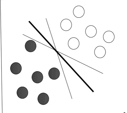
SVM were originally designed for binary classification. The basis of classification by a SVM is illustrated in Figure 1. A large number of candidate classifiers can separate the two classes shown in Figure 1 but there is only one that provides the maximum margin between the two classes and is termed the optimal separating hyperplane (OSH). Because of its definition, this classifier is expected to generalise accurately on unseen cases as compared to other classifiers.
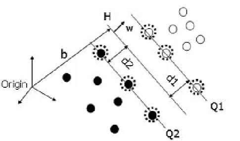
the support vectors which are fundamental to classification by a SVM. The OSH can be defined as f(x) = w.x+ b, where the parameter w determines the orientation of the hyperplane in space and b defines the bias, the distance of the hyperplane from the origin (Figure 2). When it is not possible to define the hyperplane by linear equations, the data may be mapped into a high dimensional space through some non-linear mapping which has the effect of spreading the distribution of the data points in a way that facilitates the fitting of a linear hyperplane. With this, the classification decision function becomes
) ) ( sgn( ) ( 1 b k y x f r i i i
i x x, (1)
where αi, i=1,…, r are lagrange multipliers and k(x,xi) is a kernel function. The magnitude of
αi is determined by the parameter C and lies on a scale of 0-C (Belousov et al., 2002). Further
details on SVM classification for both the linearly separable and linearly non-separable situations is given in the literature (e.g. Huang et al., 2002; Melgani and Bruzzone, 2004).
The support vectors are those training samplesxi, for which i 0. Training cases other than support vectors (αi =0) do not contribute in the formulation of the classifier (equation 1) and,
are, therefore irrelevant. Such training cases may be removed from the training set without compromising the accuracy of the classification. Thus, it is possible to derive an accurate classification from a SVM trained with only a small training set.
one-against-one strategies (Huang et al., 2002; Gualtieri and Cromp, 1998). These approaches split the multi-class problem to a set of binary problems, enabling the basic binary approach of SVM to be utilised to yield a multi-class classification. A more appropriate approach for multi-class classification, that is also less computationally demanding, may be to consider all classes at one time, yielding a multi-class SVM (Hsu and Lin, 2002). One means to achieve this, which is similar in basis to the ‘one-against-all’ approach, is by solving a single
optimisation problem. The work described hereafter is focused around one such multi-class SVM.
3 Data and methods
The study area comprised of south-western part of Punjab state of India. Indian Remote Sensing Satellite (IRS-1D) data with a spatial resolution of approximately 24 m acquired by LISS-III sensor, on 22nd September were used. The remotely sensed data were acquired in red (0.62-0.68 m), near-infrared (0.77-0.86 m) and middle-infrared (1.55-1.75 m) wavebands.
The ground data on class membership were collected by visiting the field immediately prior to image acquisition during the period 15th to 21st September, 2003. Attention focused on the dominant agricultural and non-agricultural classes in the study area. The agricultural classes were cotton, basmati rice and a local variety of rice while the non-agricultural classes were built-up land and sand.
emphasis was on the acquisition of information on crops.
A range of conventional approaches to training data acquisition can be identified, differing mainly in the detailed nature of the sampling design used. The scheme adopted here was based on a stratified random, by class, sampling design similar to that used operationally for mapping in this region within the Crop Acreage and Production Estimation (CAPE) project (Yadav et al., 1995). This approach helps ensure that even relatively rare classes, such as sand and basmati rice within the study area, are adequately sampled. The sampling process was based on a grid of 500 x 500 m size overlaid upon a map of the study area. The function of the grid was to ensure that the training data were acquired over a large geographical area, a
feature often perceived as being desirable as it helps ensure class variability is captured. Grid cells were selected at random and visited on the ground in order to locate homogeneous sites for training purposes. From each selected grid cell, one pixel was selected from the
homogeneous sites of the classes visited. In total, 180 cells were selected for each of the five classes under study. For each class, the 180 pixels acquired by this approach were divided randomly into training and testing sets. The training set, therefore, comprised 90 pixels of each class and a total of 450 pixels (Figure 3). Note that the basis of selecting 90 pixels per-class for training set was the widely promoted recommendation that a training set should comprise at least 30 times the number of discriminatory wavebands to be used in the
classification analysis. The derived training set should have captured the spectral variability of the classes and provide a full characterisation of the classes.
classification by a SVM, only the training samples that are support vectors, which lie on part of edge of the class distribution in feature space, are required; all other training samples provide no contribution to the classification analysis and can be discarded without impacting on the accuracy of the classification. To capture border training data that would act as support vectors it would be expected that attention should focus on the extremities of the class
spectral responses. With the intelligent training scheme, training data were, therefore, acquired from sites with relatively extreme spectral responses (potential border training samples) that should provide appropriate support vectors. This approach was adopted for the agricultural classes. The approach requires a basic understanding the variables affecting the spectral response of a crop (Foody and Mathur, 2004b). It is expected that these include factors related with the growth stage of the crop, the soil background and the water status of the training sites. For instance, a healthy crop generally has very high near-infrared
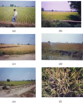
local newspaper reports and valuable information about spatial distribution of crops with regard to their type and stage of /maturity from discussion with local agricultural departments within the study area and farmers at the field level. So, the intelligent selection of training cases of the crops was directed by information on soil background properties, water status and crop growth stage. The effect of each variable on the spectral response may vary between the crops. For example, at the time of data acquisition an incomplete canopy was observed for just the cotton limiting the direct effect of variation in soil background to this crop only. Similarly, the only crop exhibiting marked variation in growth stage was the local rice crop that occurred at stages varying from young and healthy through to a very matured condition (Figure 5). Variation in water condition was linked to seepage from water bodies and specific watering activities and could affect all of the crops located in close proximity to the water network. In total, 80 training cases were identified in the field for use in the intelligently defined training set. These cases comprised 30 cases each of cotton and local rice and 20 cases of basmati rice. These sample sizes were arbitrarily selected but are considerably smaller than the 90 cases per-class acquired with the conventional scheme for training data acquisition.
The training sets derived from the conventional and intelligent data acquisition schemes were used to drive SVM classifications. The multi-class SVM approach to classification with a Gaussian kernel was used in all analyses. The parameters of the SVM were optimised for each analysis using a five-fold cross-validation approach. With the conventionally defined training set, the parameters C and γ, which controls the width of the kernel, were set at 0.25 and 0.005 respectively. With the intelligently defined training set the C and γ parameters were set at 1.0 and 0.000625 respectively.
The accuracy of each classification was assessed using the same testing set. Confusion matrices were constructed for each classification to summarize the allocations made and the accuracy, expressed in terms of the percentage of cases correctly allocated, of each
classification determined. Since each accuracy statement derived provides only an estimate of classification accuracy, it is inappropriate to simply compare the magnitude of the estimates directly in order to determine if the classifications differed in accuracy. Instead, the
classification accuracy statements derived from the analyses using the training sets acquired by the conventional and intelligent training data collection schemes were compared in a rigorous fashion that accommodated for the related nature of the samples using a McNemar test (Foody, 2004). This test that is based on confusion matrices that are 2x2 in dimension and show the level of inter-classifier agreement in correct and incorrect allocations. The McNemar test is based upon the standardised normal test statistic,
21 12 21 12 f f f f Z (2)
in which fij indicates the frequency of allocations lying in element i,j of the 2x2 confusion
mis-classified by the other. With this test, two classifications may be considered to be of different accuracy at the 95% level of confidence if Z>1.96. Thus, if the conventional and
intelligent training data acquisition schemes yielded classifications that were not significantly different, Z <1.96.
4 Results and discussion
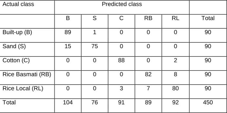
The conventionally defined training set was used to derive a classification with an accuracy of 92.00% (Table 1). This result highlights that SVM may be used to derive very accurate
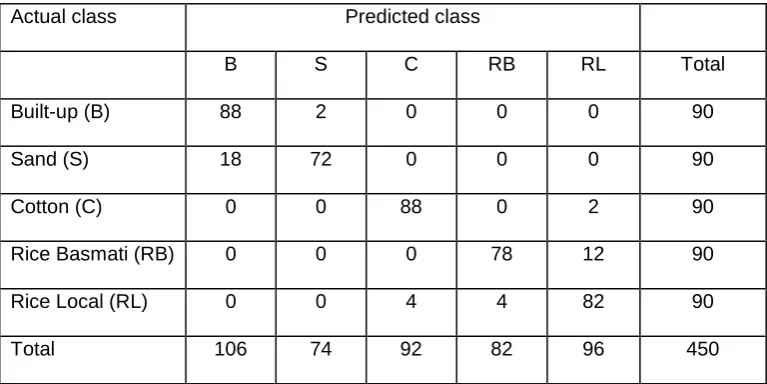
classifications. The considerably smaller, intelligently defined, training set was, however, used to derive a classification with an accuracy of 90.66%, only marginally, and
insignificantly (Z=1.50), less accurate than that derived from the conventional approach (Table 2). By focusing the training data acquisition process on the sites believed to have a high expectation of forming support vectors it was, therefore, essentially possible to use a small training set without any significant negative impact on classification accuracy. The 1.34% decrease in accuracy was achieved with a decrease in training set size from 450 (90 of each class) to 130 pixels (80 from the agricultural and 50 from the non-agricultural classes). Moreover, the reduction in training set size offers savings to the analyst. Savings in the time needed to acquire the training set as well as in costs of transportation and support of the team of fieldworkers would all be expected to result from a decrease in training set size. As a guide to the size of the savings achievable, the conventional training data acquisition scheme
38.8% and would be associated with large savings in fuel and vehicle use. These travel cost and associated savings contributed to an estimated ~26% financial saving on the total cost of producing and evaluating the crop classification through the adoption of the intelligent rather than conventional training data collection scheme (Mathur, 2005).
Attention in defining the intelligent training set was focused mainly on the identification of the most useful training sites for the discrimination of the three agricultural crop classes. It was evident that 70% of the intelligently defined training samples were support vectors. Within the conventionally defined training set the proportion of support vectors was lower, with only 41.5% of the crop training samples being support vectors (Table 3). The fieldwork, therefore, appeared to direct the training data acquisition process to the most informative locations. Moreover, from inspection of the support vectors and relation to ancillary
knowledge it may be possible to further refine the process. For example, inspection of the α values for the support vectors determined for the cotton crop showed that these had
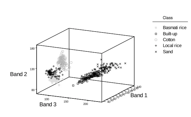
predominately come from waterlogged areas. This is unsurprising as waterlogging will reduce the reflectance of the crop and so such sites would be expected to have a reflectance closer to the local rice crop, the spectrally closest class, than cotton on dry soil (Figure 3). Indeed the only support vector for the cotton crop located on dry soil had the lowest α value, 0.6051, while all others had the maximum value of 1.0 and so actually contributed very little to the analysis. Dropping this one training case from the data set had no impact on the class
5 Conclusions
The desire in training a supervised classifier has often been to derive an accurate and
complete description of the spectral response of all the classes in the study area. To achieve a complete description of each class in feature space, a large training set is typically required. Although this may be appropriate for some classifications it is not always necessary to have training statistics that provides a complete and representative description of the classes, especially if using non-parametric classifier such as a SVM. For SVM classification, training samples are not equally important with those lying near the edge of the class distributions in feature space and facing the distributions of other classes in feature space, the support vectors, most important in the fitting of the decision boundaries between the classes. Thus, if there is some ancillary information that can be used to identify/locate training sites to regions from which the most informative training samples, the support vectors, can be derived, it may be possible to acquire a small intelligently selected training set that can be used to accurately classify the data. The study showed ancillary information on crop status and the background properties of training sites (soil type and water content) can be employed as part of the training data acquisition process in order to identify the most informative training samples, the support vectors. Relative to the use of a conventional scheme, the accuracy of the resulting classification was 1.34% less accurate at 90.66% but involved substantially less effort and could be acquired at less expense.
the conventional method. Moreover, analysis of the contribution made by each training sample to the classification showed that the intelligent training data acquisition scheme could be further refined. For example, inspection of the α values for the training cases highlighted that the most informative training samples for the cotton class were located near water bodies. Future classifications could, therefore, direct training data acquisition activities for the cotton crop to regions near water bodies and ignore other factors that influence the spectral response.
Acknowledgements
We are grateful to Dr. P.K Sharma, Director Punjab Remote Sensing Centre, Ludhiana for providing the facilities and support for field visit and data used in the study. The help rendered by Mr. P.K Litoria, Dr. D.C Loshali and Mr. Surjit Singh for field visit is also duly acknowledged. The field information provided by agriculture departments, Tribune
newspaper and the farming community in the study area is highly appreciated. The authors are also grateful to the Commonwealth Scholarship and Fellowship plan administered by the British Council for provision of a scholarship to support AM’s work at the University of Southampton while on leave from Punjab Remote Sensing Centre, India. The support vector machines were constructed with BSVM (version 2.01) software developed by Chih-Wei Hsu and Chih-Jen Lin, National University, Taipei. Finally, we are grateful to the referees for their constructive comments on the original submission.
References
variables affecting the accuracy of probabilistic, fuzzy and neural network classifications,
International Journal of Remote Sensing, 18, 785-798.
ATKINSON, P. M., 1991, Optimal ground-based sampling for remote-sensing investigations - estimating the regional mean. International Journal of Remote Sensing, 12, 559-567.
BELOUSOV, A. I., VERZAKOV, S. A. and VON FRESE J, 2002, A flexible classification approach with optimal generalisation performance: Support vector machines. Chermometrics and Intelligent Laboratory Systems, 64, 15-25.
BUCHHEIM, M. P. and LILLESAND, T. M., 1989, Semi-automated training field extraction and analysis for efficient digital image classification. Photogrammetric Engineering and Remote Sensing, 55, 1347-1355.
CAMPBELL, J. B, 2002, Introduction to Remote Sensing. Third edition, Taylor and Francis, London.
CHEN, D. M. and STOW, D., 2002, The effect of training strategies on supervised classification at different spatial resolutions. Photogrammetric Engineering and Remote Sensing, 68, 1155-1161.
CONGALTON, R. G., 1991, A review of assessing the accuracy of classifications of remotely sensed data. Remote Sensing of Environment, 37, 35-46.
CURRAN, P., 1980, Multispectral remote sensing of vegetation amount, Progress in Physical Geography, 4, 315-341.
FOODY, G. M., 2002, Status of land cover classification accuracy assessment. Remote Sensing of Environment, 80, 185-201.
FOODY, G. M., 2004, Thematic map comparison: evaluating the statistical significance of differences in classification accuracy, Photogrammetric Engineering and Remote Sensing, 70, 627-633.
FOODY, G. M. and ARORA, M. K., 1997, An evaluation of some factors affecting the accuracy of classification by an artificial neural network, International Journal of Remote Sensing, 18, 799-810.
FOODY, G. M. and MATHUR, A, 2004a, A relative evaluation of multiclass image
classification by support vector machine. IEEE Transactions Geoscience Remote Sensing, 42, 1335-1343.
FOODY, G. M. and MATHUR, A, 2004b, Toward intelligent training of supervised image classifiactions: directing training data acquisition for SVM classification. Remote Sensing of Environment, 93, 107-117.
FOODY, G. M., McCULLOCH, M. B. and YATES, W.B., 1995, The effect of training set size and composition on artificial neural network classification. International Journal of Remote Sensing, 16, 1707-1723.
FOODY, G. M., MATHUR, A., SANCHEZ-HERNANDEZ, C. and BOYD, D. S., 2006, Training set size requirements for the classification of a specific class, Remote Sensing of Environment (in press).
remote sensing classification. Proceedings SPIE, 3584, 221-232
HIXSON, M., SCHOLZ, D. and FUHS, N., 1980, Evaluation of several schemes for classification of remotely sensed data. Photogrammetric Engineering and Remote Sensing,
46, 1547-1553.
HO K.T, HULL J.J and SRIHARI S.N, 1994, Decision combination in multiple classification systems. IEEE Transactions on Pattern Analysis and Machine Analysis, 16, 66-75.
HSU, C. W. and LIN, C. J., 2002, A comparison of methods for multiclass support vector machines. IEEE Transactions on Neural Networks, 13, 415-425.
HUANG, C., DAVIS, L. S. and TOWNSHEND, J. R. G., 2002, An assessment of support vector machines for land cover classification. International Journal of Remote Sensing, 23, 725-749.
JACKSON, Q. and LANDGREBE, D. A., 2001, An adaptive classifier design for high-dimensional data analysis with a limited training data set. IEEE Transactions on Geoscience and Remote Sensing, 39, 2664-2679.
MATHER, P. M, 2004, Computer Processing of Remotely-Sensed images: An Introduction. Fourth edition, Wiley, Chichester.
MATHUR, A, 2005, Land cover classification: Refining training requirements for support vector machine classification using remotely sensed data. Unpublished Ph.D.Thesis, School of Geography, University of Southampton, Southampton.
NEUMANN, J., SCHNORR, C. and STEIDL, G., 2005, Combined SVM-based feature selection and classification, Machine Learning, 61, 129-150.
PAL, M. and MATHER, P. M., 2003, An assessment of the effectiveness of decision tree methods for land cover classification. Remote Sensing of Environment, 86, 554-565.
PAL, M. and MATHER, P. M., 2004, Assessment of the effectiveness of support vector machines for hyperspectral data. Future Generation Computer Systems, 20, 1215-1225.
VAPNIK, V. N., 1995, The Nature of Statistical Learning Theory, Springer-Verlag, New York.
WILKINSON, G. G.,1996. Classification algorithms – where next? In E. Binaghi, P. A. Brivio and A. Rampini (editors) Soft Computing in Remote Sensing Data Analysis, World Scientific, Singapore, 93-99.
YADAV, MANOJ, HOODA, R. S., MOTHI KUMAR, K. E., RUHAL, D. S., KHERA, A. P., SIGH, C. P., HOODA, I. S., VERMA, URMIL, DUTTA, SUJAY and KALUBARME, M. H., 1995, Cotton Acreage Estimation in Hissar and Sirsa Districts of Haryana using IRS LISS-I Digital Data. In Proceedings of the National Symposium on Remote Sensing of Environment With Special Emphasis on Green Revolution, (Ludhiana, P.L. Printers),pp. 30-34.
ZHUANG, X, ENGEL, B. A, LONZANOGARCIA, D. F, FERNANDEZ, R. N and
JOHNANNSEN, C. J, 1994, Optimization of training data required for neuro-classification.
Table 1. Error matrix for the classification derived using training data acquired under the conventional scheme
Actual class Predicted class
B S C RB RL Total
Built-up (B) 89 1 0 0 0 90
Sand (S) 15 75 0 0 0 90
Cotton (C) 0 0 88 0 2 90
Rice Basmati (RB) 0 0 0 82 8 90
Rice Local (RL) 0 0 3 7 80 90
Table 2. Error matrix for the classification derived using training data acquired under the intelligent scheme.
Actual class Predicted class
B S C RB RL Total
Built-up (B) 88 2 0 0 0 90
Sand (S) 18 72 0 0 0 90
Cotton (C) 0 0 88 0 2 90
Rice Basmati (RB) 0 0 0 78 12 90
Rice Local (RL) 0 0 4 4 82 90
Table 3. Number of support vectors for each of the agricultural classes in the two training sets. Note the conventional and intelligent training sets contained 270 and 80 agricultural training samples in total.
Training set
Class Conventional Intelligent
Cotton 28 11
Basmati rice 38 18
Local rice 46 27
Figure captions
Figure 1. The optimal separating hyperplane. A number of classifiers, represented by lines, can separate the two classes in the two-dimensional feature space illustrated. There is, however, only one optimal classifier, represented by the dark black line, that is expected to generalize well in comparison to other classifiers.
Figure 2. Fundamentals of SVM classification. The two classes are separated by a margin of (d1+d2) by two hyperplanes Q1 and Q2 with the optimal separating hyperplane (H) lying in between. The support vectors of the two classes are shown encircled on planes Q1 and Q2.
Figure 3. Distribution of the training data for the five classes in feature space.
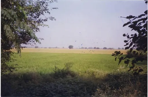
Figure 4. Variation in crop properties evident in the field that may aid the selection of support vectors prior to the classification. Note the difference between the relatively young (foreground) and mature (background) local rice crops.
140 130 120 110 100 90 80
Band 1
100
80 130
70 180
150 60
Band 2
50 200 40
Band 3
Basmati rice Built-up Cotton Local rice Sand
[image:29.595.98.406.192.381.2]Class
(a) (b)
(c) (d)
[image:31.595.127.475.69.519.2](e) (f)