Mapping long term temporal change in imperviousness using topographic maps

1

Mapping long-term temporal change in imperviousness using topographic

maps

3

James D Miller a,* & Stephen Grebby b 4

5

a _{Centre for Ecology and Hydrology, Benson Lane, Crowmarsh Gifford, Wallingford,} 6

Oxfordshire, OX10 8BB, UK 7

b _{British Geological Survey, Keyworth, Nottingham, NG12 5GG, UK} 8

9

* _{Corresponding author: Tel: +44 (0)1491 692708; E-Mail: [email protected]} 10

11 12 13 14 15

16

17

18

19

Keywords: Imperviousness; Urban; Remote Sensing; Hydrology, Land Use Change 20

2

Abstract

22

Change in urban land use and impervious surface cover are valuable sources of information for 23

determining the environmental impacts of urban development. However, our understanding of 24

these impacts is limited due to the general lack of historical data beyond the last few decades. 25

This study presents two methodologies for mapping and revealing long-term change in urban 26

land use and imperviousness from topographic maps. Method 1 involves the generation of maps 27

of fractional impervious surface for direct computation of catchment-level imperviousness. 28

Method 2 generates maps of urban land use for sub-sequent computation of estimates of 29

catchment imperviousness based on an urban extent index. Both methods are applied to estimate 30

change in catchment imperviousness in a town in the South of England, at decadal intervals for 31

the period 1960–2010. The performance of each method is assessed using contemporary 32

reference data obtained from aerial photographs, with the results indicating that both methods are 33

capable of providing good estimates of catchment imperviousness. Both methods reveal that 34

peri-urban developments within the study area have undergone a significant expansion of 35

impervious cover over the period 1960–2010, which is likely to have resulted in changes to the 36

hydrological response of the previously rural areas. Overall, results of this study suggest that 37

topographic maps provide a useful source for determining long-term change in imperviousness in 38

the absence of suitable data, such as remotely sensed imagery. Potential applications of the two 39

methods presented here include hydrological modelling, environmental investigations and urban 40

planning. 41

3

1. Introduction

45

Accurate estimates of impervious surface coverage (commonly known as 46

imperviousness) within watersheds (catchments) are required for hydrological modelling and 47

urban land use planning because increased imperviousness results in decreases in infiltration and 48

soil storage capacities (Kidd and Lowing, 1979). Furthermore, replacement of natural drainage 49

with artificial conveyance pathways can also reduce catchment response times (Packman, 1980). 50

These impacts can subsequently combine to increase the frequency and magnitude of flood 51

events through increased and more rapid runoff (Huang et al., 2008; Villarini et al., 2009), and 52

lead to disruption of natural groundwater recharge (Shuster et al., 2005; Im et al., 2012). 53

Moreover, the hydrological alterations caused by increasing imperviousness typically give rise to 54

environmental issues, such as degraded water quality, decreased biodiversity in water bodies, 55

and increased stream-bank erosion (Schueler, 1994; Arnold and Gibbons, 1996; Hurd and Civco, 56

2004; Amirsalari et al., 2013). Such impacts can be especially pronounced in peri-urban 57

developments; areas surrounding existing towns, which convert previously permeable rural land 58

into highly impermeable and artificially drained catchments (Tavares et al., 2012).Understanding 59

and modelling the long-term hydrological impacts of increased urban development requires 60

concurrent information on the change in impervious surface coverage. Maps of impervious 61

surfaces can be produced from either field surveys, manually digitising from hard-copy 62

topographic maps, or the use of remote sensing (RS) data. Whereas field surveys and manual 63

digitisation can be time-consuming and laborious, the large continuous areal coverage provided 64

by RS datasets can be exploited using image processing algorithms to rapidly map impervious 65

surfaces for only a fraction of the time and cost. Accordingly, RS is becoming increasingly 66

4

review of the different methodologies employed to map impervious cover from RS data is 68

provided by Weng (2012). To summarise, RS-based approaches to mapping imperviousness 69

generally fall into three broad categories: per-pixel, object-based and sub-pixel. Per-pixel 70

approaches commonly involve producing a binary map by determining whether individual image 71

pixels correspond to either pervious or impervious surfaces, typically through aggregating the 72

classes of an initial land cover classification (Yuan and Bauer, 2006; Im et al., 2012; Amirsalari 73

et al., 2013). In contrast, object-based approaches involved the classification of groups of 74

contiguous image pixels (i.e., objects or regions) by also considering various shape, contextual 75

and neighbourhood information (Benz et al., 2004; Weng, 2012). Classifying an image based on 76

objects helps to overcome the “speckled” effect often encountered with per-pixel classification in 77

urban areas (Van de Voorde et al., 2003), thus enabling improved mapping results (Yuan and 78

Bauer, 2006; Zhou and Wang, 2008). A major limitation of per-pixel approaches is that they 79

assume each pixel comprises a single land use or land cover type. However, pixels containing a 80

mixture of land use or cover types are common in low-to-moderate resolution imagery acquired 81

over complex heterogeneous landscapes such as urban areas (Weng, 2012). Sub-pixel 82

approaches can be used to overcome this to derive accurate estimates of imperviousness because 83

they decompose the pixel spectra into their constituent parts, therefore providing fractional 84

measures of impervious surface area. Popular approaches in this category include unmixing the 85

pixel spectra to determine the fractional abundance of each constituent end-member surface type 86

(Lu et al., 2006), or modelling fractional imperviousness through statistical regression and 87

scaling of spectral vegetation indices (Bauer et al., 2004; Van de Voorde et al., 2011).With the 88

earliest source of RS data comprising panchromatic aerial photograph lacking in sufficient 89

5

decades since the emergence of spectral satellite imagery (e.g., Landsat). Consequently, few 91

studies have assessed long-term land cover change using RS data (e.g., Gerard et al., 2010; 92

Tavares et al., 2012), and even fewer have mapped long-term changes in impervious cover 93

(Weng, 2012). Therefore, our understanding of the hydrological impact and non-stationary 94

flooding trends in relation to impervious surface change is somewhat limited (Ogden et al., 2011; 95

Vogel et al., 2011; Dams et al., 2013). Linking imperviousness to alternative sources of digital 96

geo-information could provide a means of mapping long-term changes in impervious cover. 97

However, such datasets are not usually available at the national scale or comparable over long 98

periods of time. National land cover mapping products such as the UK Land Cover Map (LCM) 99

1990, 2000 and 2007 (Centre for Ecology and Hydrology) cover only a short time period and are 100

inconsistent due to the different processing algorithms applied to derive each product from the 101

RS data (Morton et al., 2011). While methods such as land use trajectory analysis (Verbeiren et 102

al., 2013) could be applied to help improve the consistency of the time-series somewhat, there 103

will still likely be a residual error arising from the use of contrasting algorithms for generating 104

each data product. Physical settlement boundaries and land use change statistics may be a useful 105

alternative source of information (e.g., Bibby, 2009) but can only be loosely regarded as proxies 106

for imperviousness. In most cases, the only consistent and long-term sources are topographic 107

maps produced by national agencies. Within the UK topographic maps have been produced by 108

the Ordnance Survey — the national mapping agency for Great Britain — since the mid-19th 109

century. Despite representing a potentially valuable source for deriving long-term change in land 110

use or land cover, studies assessing the use of such information are scarce (e.g., Hooftman and 111

Bullock, 2012). The aim of this study is to utilise historical topographic maps for semi-112

6

methods are presented that utilise topographic maps to: (i) derive maps of fractional impervious 114

surface for direct computation of catchment-level imperviousness; (ii) derive maps of urban land 115

use for subsequent computation of estimates of catchment-level imperviousness based on an 116

urban extent index. Impervious surface cover estimates computed using these two methods are 117

validated using reference data generated through a RS-based image classification of high-118

resolution aerial photographs. The methods presented herein are employed in an attempt to 119

determine their suitability for indicating change in urban land use and imperviousness — here 120

throughout a 50-year period from 1960 to 2010 in a number of hydrological catchments 121

surrounding a UK town that exemplifies rapid peri-urban development. 122

123 124

2. Study area

The study area (Fig. 1) encompasses two adjacent small urban stream catchments located 126

to the north of Swindon in the south of England; comprising the Haydon Wick brook and 127

Rodbourne stream, both tributaries of the River Thames (Fig. 1 inset). Swindon was designated 128

as an Expanded Town under the Town Development Act in 1952 which encouraged town 129

development in county districts to relieve over-population elsewhere. The Rodbourne stream 130

catchment has been highly urbanised since the 1950s and comprises a large area of commerce 131

and industry on the northern edge of Swindon town, along with highly urbanised housing 132

developments. The Haydon Wick brook catchment is located further to the north of Swindon and 133

has undergone widespread development since the 1990s, prior to which it was a predominantly 134

agricultural landscape. Within the Haydon Wick catchment a number of distinct catchments (1– 135

7

developments within the area. The Rodbourne catchment, in which development has 137

incrementally expanded since the 1950s, remains one single catchment unit (6) for this study. 138

The focus of this study is to test two methodologies for mapping changes in urban land use and 139

associated imperviousness in each of these six catchments during the period 1960 to 2010.3. 140

141

Fig. 1. Map of the study area showing catchment boundaries and location of the study area within 142

the Thames Basin (inset). RGB aerial photography – © UK Perspectives: License Number 143

UKP2006/01. 144

145

8 147

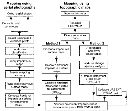
Fig. 2. Overview of methodological approach used to assess the utility of traditional topographic 148

maps for long-term, historical mapping of urban extent and estimation of catchment 149

imperviousness. 150

151

152

3.

Material and methods

153

The ability to utilise traditional topographic maps for long-term, historical mapping of 154

urban extent and estimation of catchment imperviousness is assessed using a three-pronged 155

approach (Fig. 2). The approach involves first estimating contemporary catchment fractional 156

impervious surface area directly from aerial photographs for use as reference data. These 157

9

historical change in impervious cover topographic maps. Following validation, a comparison of 159

the two methods is undertaken to assess their relative performance revealing long-term change in 160

catchment impervious cover between 1960 and 2010. More detailed information regarding the 161

methodological approach is provided in the following sub-sections. 162

163

3.1 Deriving catchment imperviousness from aerial photographs 164

Reference data for quantifying the catchment fractional impervious cover were obtained 165

from aerial photographs for three decadal time-slices within the 50-year period of interest — 166

namely 1991, 1999 and 2010 (herein referred to as 1990, 2000 and 2010, respectively). The 167

reference data were generated by first classifying 0.5 m true-colour aerial photographs into 168

pervious land cover classes: grass, trees, bare soil and water; and impervious land cover classes: 169

roads/pavements, commercial buildings and residential buildings. It was anticipated that land 170

cover classes such as bare soil and roofing tiles could be particularly difficult to discriminate 171

using the limited spectral information contained in only the red, green, blue bands of the aerial 172

photographs. Therefore, textural information was also incorporated in the form of the Grey-Level 173

Co-occurrence Matrix (GLCM) parameters of entropy, dissimilarity, second moment and 174

homogeneity (Haralick et al., 1973; Herold et al., 2003). These parameters were derived from the 175

green band in the ENVI 4.8 software package (Research Systems, Inc.) for a 3 × 3pixel (i.e. 1.5 176

m × 1.5 m) window and a co-occurrence window shift of 4 pixels (i.e., 2 m) in both the x- and y-177

direction. This combination of window size and shift was chosen as it maximised visual 178

discrimination of the different land cover classes. Classification of the three time-slices 179

employed a neural network (NN) classification algorithm in conjunction with the seven 180

10

producing better classification results for complex heterogeneous urban areas than their 182

conventional counterparts (e.g., Maximum Likelihood), since they are non-parametric and more 183

robust in handling noisy and non-normally distributed data (Foody, 2002). The NN used in this 184

case was a Multi-Layered Perceptron NN with a back-propagation learning algorithm for 185

supervised learning (Richards and Jia, 2006). Using a three-layered NN (i.e., input, output and 186

one hidden layer), land cover classifications were performed in ENVI 4.8 with the default 187

training parameters confirmed through a set of trial-and-error experiments. Each classification 188

was supervised with the aid of a set of training pixels that were carefully selected in the imagery 189

to represent each of the defined land cover types (∼6000 pixels for each class). Land cover 190

classifications were converted to binary imperviousness maps by collapsing the classes into just 191

two corresponding to pervious or impervious surfaces (Yuan and Bauer, 2006; Im et al., 2012; 192

Amirsalari et al., 2013). The accuracies of the resulting binary imperviousness maps were 193

determined by comparing the true class identities of a sample of validation pixels to the classes 194

assigned through classification. Validation pixels were selected from regions of interest (ROIs) 195

of known pervious or impervious surface class identities that were defined in each time-slice 196

image based on extensive knowledge of the study area. Validation pixels were then selected from 197

the ROIs using a random stratified sampling protocol to ensure each class was represented 198

proportionately, and to avoid spatial autocorrelation within the validation dataset (Chini et al., 199

2008; Pacifici et al., 2009). The minimum validation sample size required to derive statistically 200

valid accuracy estimates for the entirety of each binary map was determined from the normal 201

approximation of the binomial distribution (Fitzpatrick-Lins, 1981). Consequently — based on 202

11

approximately 19,000 validation pixels for each class were selected to determine the accuracy of 204

each binary imperviousness map. 205

Binary imperviousness map accuracies were assessed by way of the overall (OA), user’s 206

(UA) and producer’s (PA) accuracies and the Kappa coefficient (K) derived from a confusion 207

matrix (Congalton, 1991). The overall accuracy is the percentage of all validation pixels 208

correctly classified, whereas the user’s and producer’s accuracies provide information regarding 209

the commission and omission errors associated with the individual classes, respectively. 210

Following validation, the 0.5 m binary impervious maps were aggregated to 50 m grid cells to 211

generate fractional impervious surface maps, with the value for each grid cell corresponding to 212

the proportion of impervious pixels within it. The value of 50 m was selected as it was found to 213

best represent homogeneous scale of urban land use classification (see Section 3.2.2). The 214

imperviousness of each of the six catchments (%IMP) was then computed from these fractional 215

impervious surface maps for use as reference data, using: 216





c n

i

i i

A A IMP IMP



 %

% , (1)

217

where %IMPi is the fractional impervious cover for grid cell i, Ai is the area of the grid cell, n is

218

the number of grid cells within the catchment, and Ac is the total catchment area.

219 220

3.2 Deriving estimates of catchment imperviousness using topographic maps 221

As outlined in Fig. 2, estimates of catchment fractional impervious surface cover were 222

derived using two methods. In general, these consist of first generating binary imperviousness 223

12

fractional imperviousness maps or urban land use maps — as illustrated in Fig. 3 and described 225

below. 226

227

3.2.1 Data and pre-processing 228

Digital historical topographic maps produced by the UK Ordnance Survey (OS) between 229

1960 and 2010 were obtained in raster format as 25 km × 25 km tiles with a 1 m spatial 230

resolution. For each decade (1960s to 2010s), the most contemporaneous map tiles produced for 231

that decadal time-slice were obtained and mosaicked to produce a seamless image for each 232

decade (Table 1). The primary step for the two methods is to convert the historical topographic 233

maps into simplified and physically representative binary maps of developed (i.e., impervious) 234

and undeveloped (i.e., pervious) pixels. To do this, the original pixel values were reclassified so 235

that a value of 1 was assigned to pixels corresponding to ‘white space’ on the map and a value of 236

2 to all pixels corresponding to mapped features. 237

238

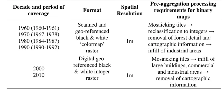
Table 1. Ordnance Survey mapping data and pre-processing requirements. 239

Decade and period of

coverage Format

Spatial Resolution

Pre-aggregation processing requirements for binary

maps 1960 (1960-1961) 1970 (1967-1978) 1980 (1984-1987) 1990 (1990-1992) Scanned and geo-referenced

black & white ‘colormap’

raster

1m

Mosaicking tiles →

reclassification to integers → removal of forest detail and cartographic information → infill of industrial areas

2000 2010

Digital geo-referenced black

& white integer

raster 1m

Mosaicking tiles → infill of large buildings, commercial

and industrial areas → removal of cartographic

information 240

13 242

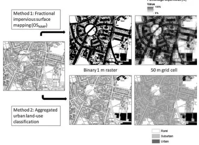
Fig. 3. Illustration of the approach applied in both method 1 and 2 to map impervious cover. 243

Topographic base map – © Crown copyright and Landmark Information Group. 244

245

Due to slight variations in the cartographic style used from 1960 to 2010, a number of 246

steps were required to further improve the consistency and compatibility of each map. The first 247

stage involves developing ‘level-1’ binary maps, in which artefacts and key inconsistencies 248

between maps from each decade are reduced. This was undertaken using the ‘Raster Cleanup’ 249

tool in ArcMap (ArcGIS 10, ESRI) and included the following steps: 250

 A rapid ‘clean-up’ of each raster map is undertaken to remove features, such as 251

place names or symbols relating to widespread forest; 252

 Reclassifying large concrete or tarmac areas represented by ‘white space’ to 253

14

 Infilling the roofs of large buildings on raster maps for 2000–2010due to the low 255

density of pixels used to represent such areas on these maps. 256

257

A second pre-processing stage was subsequently applied for the purpose of infilling 258

developed features such roads and buildings to generate a set of ‘level-2’ binary maps. This was 259

undertaken in ArcMap by applying the ‘Boundary Clean’ tool to each raster and then converting 260

them to polygon shapefiles. This conversion enables road segments and buildings to be readily 261

reattributed to alter them from polygons representing pervious (undeveloped) features to 262

impervious (developed) features. Once all relevant polygons have been reassigned, the shapefiles 263

were then converted back to raster format. 264

265

3.2.2 Deriving catchment imperviousness from fractional impervious surface maps 266

The first method (method 1) for deriving catchment imperviousness for the six 267

catchments is relatively straightforward to implement, and is focussed on the generation of 268

fractional impervious surface maps of the study area. To generate these maps, the ‘level-2’ 269

binary maps derived from the topographic maps were aggregated to 50 m grid cells in a similar 270

manner to that used to derive fractional impervious surface maps from the aerial photographs. In 271

this case, the value for each 50 m grid cell is calculated as the proportion of 1 m impervious 272

pixels contained within it. Although pre-processing steps were implemented to improve the 273

compatibility and consistency of the topographic map time series (1960–2010), additional 274

calibration was performed to account for any residual discrepancies between the fractional 275

impervious surface maps. Adopting the approach outlined by Lu et al. (2011), pseudo-invariant 276

15

were selected for pair-wise image calibration via linear regression models. As a result, all 278

fractional impervious surface maps were calibrated to the most recent map (i.e., 2010). Once 279

calibrated, the imperviousness of each of the six catchments (OS%IMP) is computed from these

280

calibrated fractional impervious surface maps using an adaptation of Eq. (1), and compared with 281

the contemporaneous reference data derived from aerial photography (%IMP). 282

283

3.2.3 Deriving catchment impervious cover from urban land use maps 284

The second method (method 2) for deriving catchment imperviousness for the six 285

catchments is based on the generation of urban land use maps from the topographic maps. Maps 286

of urban land use were generated by aggregating the topographic map-derived binary maps for 287

each decade to larger grid cells, and then classifying the cells according to the LCM land 288

use/land cover definitions; mixed development and green space designated as Suburban (e.g., 289

houses with gardens), areas of near continuous development with little vegetation (e.g., industrial 290

estates) designated continuous Urban (Fuller et al., 2002), and all other areas of green and 291

general pervious surfaces referred to as Rural. Following a preliminary evaluation of a number of 292

different grid cell sizes, a cell size of 50 m was identified as the optimum for generating realistic, 293

homogeneous urban land use maps; smaller cell sizes produced maps with the aforementioned 294

‘speckled’ effect that often affects per-pixel classification in urban areas. Additionally, it was 295

found that application of this approach to the ‘level-2’ binary grids resulted in difficulty devising 296

a standard classification which can be used to produce coherent land use maps across the time 297

series. For this reason, the ‘level-1’ binary maps derived from the topographic maps were used to 298

generate the land use maps. This was achieved using ArcMap through the following steps: 299

16

 ‘Level-1’ binary maps were aggregated using the ‘Aggregate’ function to generate a 301

grid that details the mean value of the pixels contained within each 50 m grid cell. 302

These aggregated values provide an indication of the level of development; 50 m grid 303

cells with a value close to 1 essentially correspond to ‘white space’ (i.e., a rural 304

undeveloped area), whereas a value close to 2 corresponds to a high density of 305

mapped features (i.e., a highly developed area). 306

 A threshold-based classification scheme was then applied to the grid in order to 307

assign cells to either the Urban, Suburban or Rural land use class. It was found that 308

cell values of 1–1.35 represented Rural land use, values of 1.35–1.65 corresponded to 309

Suburban, and values above 1.65 represented Urban land use. These thresholds were 310

validated to ensure at least 80% of 50 randomly selected grid cells were correctly 311

classified in decadal map. The output is set of 50 m maps showing Rural, Suburban, 312

and Urban land use (shown in Fig. 3). 313

Potentially erroneous pixel classifications were removed through geospatial proximity 314

analysis, and by applying an urban land use change trajectory demonstrated by Verbeiren et al. 315

(2013) to ensure greater consistency throughout the time series. This is achieved by first 316

combining the ArcGIS ‘Conditional’ tool in the ‘Raster Calculator’ with the ‘Focal Statistics’ 317

tool to identify misclassified Urban and Suburban grid cells based on the classes of neighbouring 318

cells — isolated Suburban or Urban cells were reclassified according to the dominant 319

surrounding class. Following this, each cell was labelled as either 0 (Rural), 1 (Suburban) or 3 320

(Urban) and all trajectories of land use change were recorded throughout the time series using 321

codes (e.g., 00112, 01222, etc.). These were then evaluated according to whether they reflect 322

17

into 6 rationality classes: ‘urban growth’, ‘suburban growth’, ‘urban regeneration’, ‘urban 324

stability’, ‘suburban stability’, and ‘inconsistent’. The ‘inconsistent’ class captures grid cells that 325

do not follow realistic change trajectories — such as a Suburban area changing to Rural then 326

Suburban and back to Rural. Inconsistent cells were corrected using the most likely trajectory for 327

that cell over the 50-year period — based upon surrounding cells. The class ‘urban regeneration’ 328

captures the possibility of Urban areas being demolished and replaced with green space or 329

subsequent re-development. The land use change trajectory rules were implemented using the 330

‘Conditional’ tool in the ArcMap ‘Raster Calculator’. The outcome was as set of coherent urban 331

land use maps revealing the long-term change in land use for the period 1960–2010. 332

For each land use map, the proportions of Urban and Suburban grid cells within each 333

catchment were used to calculate a catchment index of urban extent. As well as measuring the 334

urban extent within a hydrological catchment, the index of urban extent (URBEXT) proposed in 335

the UK Flood Estimation Handbook (FEH) methodology (Institute of Hydrology, 1999) can also 336

provide an estimate of the impervious surface cover. Accordingly, the index of urban extent and 337

estimate of imperviousness for the six catchments (URBEXT) in each land use map is computed 338

using: 339





Urban

URBEXT  



where Urban and Suburban are the proportions of Urban and Suburban grid cells within each 341

catchment, respectively, and β is the Suburban weighting factor. The suitability of URBEXT for 342

estimating catchment imperviousness is assessed through comparison with the reference data 343

derived from aerial photography (%IMP). For the purpose of this comparison, URBEXT — the 344

weighted value of urban extent within a catchment — is considered to provide a direct estimate 345

18

value of 0.5 to account for the general equal mixture of built-up land and permanent vegetation 347

(Bayliss et al, 2006; Institute of Hydrology, 1999). Urban land use was assigned a weighting of 1 348

because such areas generally have negligible green (pervious) space. In an attempt to improve 349

the accuracy of the catchment imperviousness estimates, an optimal value for β was sought by 350

applying a linear regression model between reference imperviousness (%IMP) and URBEXT 351

across the three decadal time-slices. This provides a refined calibrated value of catchment 352

impervious surface (URBEXTIMP).

353 354 355

4. Results and discussion

4.1 Imperviousness maps from aerial photography 357

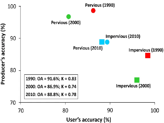
The accuracies of the RS-derived high-resolution (0.5 m) maps of binary imperviousness 358

for 1990, 2000 and 2010 are shown in Fig. 4. High overall accuracies (>86%) were achieved in 359

all three cases and are also confirmed by the corresponding K values (0.74–0.83); interpreted as 360

reflecting a “substantial” to “almost perfect” degree of accuracy (Landis and Koch, 1977). 361

Further corroboration of the classification accuracy is provided by the high user’s (88–99%) and 362

producer’s (77–89%) accuracies associated with both the pervious and impervious classes in all 363

binary imperviousness maps; indicating low commission and omission errors, respectively. The 364

result of this accuracy assessment indicate that the binary imperviousness maps are suitable for 365

deriving reference data for validating the estimates of catchment imperviousness computed using 366

the topographic map-based methods. 367

19 370

371

Fig. 4. Classification accuracies of the binary imperviousness maps derived from aerial 372

photographs for 1990, 2000 and 2010. OA — Overall accuracy; K — Kappa coefficient. 373

374

4.2 Catchment imperviousness from fractional impervious surface maps 375

Catchment imperviousness obtained from topographic map-derived fractional impervious 376

surface maps (OS%IMP) — method 1 — was compared with the reference data (%IMP) derived

377

from the aerial photographs (Fig. 5). A reasonable, but variable level of agreement between 378

OS%IMP and %IMP is observed throughout the three decadal time-slices. Although the correlation

379

for 1990 is greatest (R2 = 0.96), the catchment imperviousness measured using OS%IMP is (with

380

the exception of catchment 3) approximately 10% larger than the reference data. The general 381

overestimation of OS%IMP is most likely attributable to the larger size depictions of features such

382

as roads on the 1990 topographic map, compared to equivalent features on the more recent maps. 383

The correlation between OS%IMP and %IMP is somewhat lower for both 2000 and 2010 (R2 =

384

0.75 and 0.62, respectively), with the data appearing more widely distributed around the 385

20

the exact instant in time at which the aerial photographs and corresponding topographic maps 387

capture. Alternatively, this could arise due to the slightly lower accuracies of the 2000 and 2010 388

aerial photography-derived binary imperviousness maps, in comparison to the 1990 map. 389

Nevertheless, the results suggest that estimating catchment imperviousness using fractional 390

impervious surface maps derived from topographic maps (i.e., method 1) is feasible. 391

392

393

Fig. 5. Comparison of catchment imperviousness estimated from aerial photography (%IMP) and 394

topographic map-derived fractional impervious surface cover (OS%IMP) within the six catchments, 395

for years 1990, 2000 and 2010. 396

397

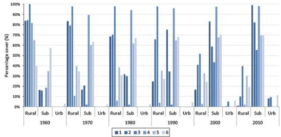
4.3 Mapping urban land use change using topographic maps 398

Urban land use derived from the topographic maps using method 2 reveals the spatio-399

temporal change in Urban, Suburban and Rural land use at a decadal intervals from the 1960s to 400

2010s (Fig. 6). While the highly urban Rodbourne catchment (catchment 6) exhibits a gradual 401

expansion and infilling of Urban and Suburban land use, the Haydon Wick catchments (1–5) 402

exhibit a more dramatic and rapid changes in land use over the 50-year study period. The 403

remarkable change from predominantly Rural (agricultural) land use in all Haydon Wick 404

catchments (1–5) to predominantly Suburban land use is clearly illustrated in Fig. 7, as is the 405

21

that occurred in catchment 6, which was already over 50% Suburban in 1960, is significantly less 407

than in the peri-urban area of the Haydon Wick catchments (Fig. 7). In all cases, the mapped 408

spatio-temporal changes in Urban land use were found to be consistent with the physical changes 409

observed in the original OS topographic maps. By the 2010s, the relative proportion of 410

developed (i.e., Urban or Suburban) land across all catchments is high and the remaining Rural 411

areas typically represent areas of green space designated for recreation and conservation, along 412

with areas of significant flood risk. 413

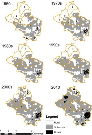
414

415

22 417

418

Fig. 7. Spatio-temporal change in urban land use across the study area. 419

420

421

422

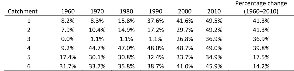
23

Table 2. Change in urban extent index (URBEXT) for the six catchments. 424

Catchment 1960 1970 1980 1990 2000 2010

Percentage change (1960–2010) 1 8.2% 8.3% 15.8% 37.6% 41.6% 49.5% 41.3% 2 7.9% 10.4% 14.9% 17.2% 29.7% 49.2% 41.3% 3 0.0% 1.1% 1.1% 1.1% 26.8% 36.9% 36.9% 4 9.2% 44.7% 47.0% 48.0% 48.7% 49.0% 39.8% 5 17.4% 30.1% 30.8% 32.4% 33.7% 34.9% 17.5% 6 31.7% 33.7% 35.8% 38.7% 41.0% 45.9% 14.2% 425

Catchment values of URBEXT computed using the land use maps (Table 2) also show 426

distinct differences between the Haydon Wick catchments (1–5) and Rodbourne catchment (6). 427

During the period 1960–2010, URBEXT values changed little across the Rodbourne catchment, 428

with only a 14.2% increase as a result of small, steady incremental change during each decade. 429

More significant change across the Haydon Wick catchments reflects successive waves of peri-430

urban development during the study period, with an average overall increase in URBEXT of 431

35.4% and significant variation between the catchments (17.5–41.3%). Again, the observed 432

temporal changes in urban extent were found to be consistent with known physical changes that 433

occurred within the period 1960–2010. Therefore, the results demonstrate that the employed 434

method is an effective approach for readily mapping long-term basic land use change and 435

associated catchment-level urban extent from historical topographic maps. A particular important 436

stage in this methodology is the application of land use trajectory analysis (e.g., Verbeiren et al., 437

2013), which was crucial in ensuring a reliable time series dataset from which only genuine land 438

use change is revealed. 439

440

4.4 Catchment imperviousness from urban land use maps 441

To investigate whether a simple index of urban extent (URBEXT) derived from 442

24

comparison with reference imperviousness derived from aerial photography (%IMP) was 444

undertaken (Fig. 8). Overall, a high correlation between URBEXT and %IMP is observed across 445

most catchments during the three decades (R2 = 0.80–0.96), and also when all data is considered 446

collectively (R2 = 0.86). Nevertheless, some notable deviations were observed for specific 447

catchments and time-slices. For example, values of %IMP for catchment 3 were shown to be 448

much higher than URBEXT in all cases due to significant underestimation of Urban areas of 449

gravel and tarmac because of their depiction on topographic maps. Also, for 1990, URBEXT 450

values are clustered around %IMP, while URBEXT consistently underestimates catchment 451

imperviousness for both 2000 and 2010. The general underestimation of catchment 452

imperviousness is likely to relate to the use of the ‘level-1’ binary grids, in which buildings and 453

roads are not infilled. Nonetheless, it is apparent that land use maps generated from topographic 454

maps can be used in conjunction with the urban index, URBEXT, (i.e., method 2) to generate 455

feasible estimates of catchment imperviousness. 456

457

458

Fig. 8. Comparison of catchment imperviousness estimated from aerial photography (%IMP) and 459

topographic map-derived index of urban extent (URBEXT) within the six catchments, for years 460

1990, 2000 and 2010. 461

25

A linear regression model between URBEXT and %IMP across the three decadal time-463

slices returned an optimised Suburban weighting factor (β = 0.53). Calibrated values of urban 464

extent (URBEXTIMP) for each catchment were computed for 1990, 2000 and 2010 by using this

465

optimised value for β in Eq. (2). Following a comparison, the overall correlation between 466

URBEXTIMP and %IMP (R2 = 0.84) was actually found to be marginally lower than for URBEXT

467

(R2 = 0.86), indicating that the original preset β (0.5) was more appropriate in this particular case. 468

However, in regions where Suburban land use does not comprise equal mixtures of built-up land 469

and vegetation, the optimal weighting can be determined using the same approach as that used 470

here. 471

472

4.5 Historical change in imperviousness 473

The two methods employed in this paper for computing catchment imperviousness from 474

topographic maps both provide a means of revealing long-term change in imperviousness. As 475

illustrated by Fig. 9, the overall trend in imperviousness change for 1960–2010 is consistent 476

between the two methods. With the exception of catchment 6, which was already highly 477

developed prior to 1960, all catchments experience a somewhat rapid increase in imperviousness 478

during a specific period between 1960 and 2010. For example, catchment 1 sees its biggest 479

increase in imperviousness during 1980–1990, while catchment 3 experiences a rapid rise during 480

1990–2000. The timings of these rapid increases in imperviousness coincide with known 481

episodes of peri-urban expansion within the study area, and reflect the pattern of continuous 482

growth and expansion where as one development finishes another one commences. The less 483

26

suburban housing stock in 1960 and that it also contains a large nature reserve which is protected 485

from development. 486

487

Fig. 9. Change in impervious cover determined using two methods across the six study catchments 488

(1960–2010). 489

490

In addition to displaying similar trends, the two methods provide very similar estimates 491

of the total absolute change in catchment imperviousness between 1960 and 2010. The mean 492

difference in the total absolute change estimates between the two methods, for all catchments, is 493

2.9%, with individual catchment estimates varying between a maximum difference of 7.1% and a 494

minimum of 0.4%. The maximum difference is associated with catchment 6, which is arguably 495

the most complex in terms of land use change during 1960–2010 because of gradual expansion 496

of the industrial area in the south-eastern section of the catchment, and regeneration of the 497

railway network to suburban housing in the south-west. As illustrated by Fig. 9, the more rural 498

northern catchments (i.e., 1–4) experienced the most significant total absolute change in 499

27

These estimates clearly reflect the rapid expansion of suburban land use into these previously 501

rural areas as revealed in Fig. 6. 502

Although Fig. 9 illustrates that the methods reveal similar trends and estimates of change 503

in imperviousness across the six catchments for 1960–2010, there are differences in the 504

individual catchment imperviousness estimates. Specifically, all estimates computed using 505

method 1 (OS%IMP) exceed those produced using method 2 (URBEXT), with a mean absolute

506

difference of 7.8% (Table 3). With respect to the time intervals, the largest differences between 507

the methods occurs for the years 1990 and 2000,where OS%IMP estimates are respectively 8.3%

508

and 9.4% greater than the equivalent URBEXT estimates. With respect to catchments, the largest 509

differences between methods are observed for catchments 5 and 6, for which OS%IMP estimates

510

are respectively 9.0% and 9.5% greater than URBEXT estimates. The overall trend of method 1 511

producing higher estimates than method 2 is explained by a combination of the contrasting 512

representation of features such as roads and buildings in the different binary maps (i.e., the level 513

of infilling) incorporated in the two methods, and the somewhat simplistic discrete weighting 514

system employed in method 2. In particular, the infilling of features such as roads in the level 1 515

binary maps used in method 1 can lead to overestimation of impervious cover as the symbology 516

used represent roads does not always reflect the true physical dimensions, and can lead to infill 517

of isolated areas that are not physically developed. Despite the fundamental differences in the 518

two methods, both have been demonstrated to be feasible approaches for computing catchment 519

28

Table 3. Absolute difference (OS%IMP – URBEXT) in estimates of imperviousness cover using two 521

topographic map-based methods. 522

523 524

4.6 Considerations in using topographic maps for estimating imperviousness 525

This paper demonstrates, through two methods, that topographic maps can be used to 526

compute estimates of catchment imperviousness. When contemplating the use, or evaluating the 527

performance, of OS%IMP and URBEXT — or any other topographic map-based method — there

528

are a several aspects that require some consideration: 529

I. Aerial photographs and topographic maps do not necessarily represent the exact same 530

instant in time, since whereas aerial photographs provide a snapshot for a specific 531

date, topographic maps incorporate updates within a given time period (see Table 1). 532

II. Failure to remove place names and symbols (e.g., to represent forests) from the 533

topographic maps will translate to the subsequently derived binary maps and lead to a 534

degree of overestimation of imperviousness – users should ensure some consistent 535

criteria are outlined for any manual interventions. 536

III. Topographic maps do not readily discriminate areas of inland bare ground and 537

concrete/tarmac features, which will subsequently lead to their misrepresentation on 538

derived binary impervious surface maps and result in a degree of underestimation of 539

imperviousness. However, infilling of features such as roads can lead to 540

Year 1 2 3 4 5 6 Mean difference

1960 8.0 8.2 5.5 5.4 9.3 10.4 7.8

1970 4.7 9.1 3.8 6.4 10.2 10.3 7.4

1980 6.3 9.0 4.6 4.3 9.0 11.1 7.4

1990 9.2 8.3 3.4 7.5 9.8 11.6 8.3

2000 12.0 7.4 7.1 11.0 8.7 10.0 9.4

2010 10.3 7.8 3.3 8.3 6.8 3.3 6.6

29

overestimation of impervious cover if the symbology used does not directly reflect 541

true physical dimensions. 542

IV. Small-scale features (e.g., minor roads) and minor changes within existing 543

development boundaries (e.g., infilling or ‘urban creep’) shown on aerial photography 544

are not always captured using the discrete land use classification and scale employed 545

in method 2. 546

V. Calibration of the fractional impervious surface maps (as in method 1) and 547

implementation of land use trajectory analysis (method 2) are crucial steps in 548

producing a coherent time series dataset for revealing reliable long-term change in 549

imperviousness. 550

With both methods capable of providing good estimates of catchment imperviousness, 551

the most appropriate method is largely dependent on the purpose of the study and the format of 552

the topographic maps. In general, method 1 can be more readily implemented and provides maps 553

of fractional impervious surfaces, thus describing imperviousness on a continuous scale (Fig. 554

10). On the other hand, despite method 2 providing only a discrete description of imperviousness 555

(see Fig. 10), it does provide maps of general land use that are informative when interpreting 556

changes in imperviousness over time. Although method 1 can be readily applied to any study 557

area, as demonstrated here, method 2 can be calibrated to determine the optimal weighting factor 558

associated with Suburban land use (β). Additionally, if the available topographic maps depict 559

roads and building as infilled features (akin to the ‘level-2’ binary maps) then method 1 would be 560

more suitable. However, if — as in the case of the OS topographic maps used here — such 561

features are not infilled, then method 2 can be applied without the need of additional pre-562

30 564

565

Fig. 10. A comparison of impervious surface maps obtained using the two methods. 566

567

5. Conclusions

This paper demonstrates that it is possible to derive robust long-term estimates of 569

catchment imperviousness from topographic maps using two different contrasting methods. The 570

first method (method 1) generates fractional impervious surface maps from the topographic maps 571

and uses these to estimate catchment imperviousness. The second method (method 2) generates 572

31

imperviousness from these using an index of urban extent. Although some degree of manual 574

intervention is required for both methods, the processing stages employed are largely semi-575

automatic and require significantly less time than manual delineation of impervious surfaces. 576

Such manual intervention will rely on some degree of user subjectivity — related to the format 577

of the topographic maps — that could alter the binary map sand derived impervious cover 578

products. Such interventions are required to produce more consistent mapping products for 579

derivation of binary maps, and it is recommended that users employ transparency in the reporting 580

of such interventions. Through comparison with reference data obtained using aerial 581

photographs, it is demonstrated that both methods are capable of providing accurate estimates of 582

catchment imperviousness and its change over time. With both methods capable of providing 583

good estimates of catchment imperviousness, the most appropriate method beyond this study will 584

be largely dependent on the purpose of the study and the format of the topographic maps. 585

This study demonstrates that both methods show the peri-urban Haydon Wick catchment 586

has undergone a significant change from predominantly rural to highly urban and is now 587

dominated by suburban areas of housing development. Findings from hydrological studies (e.g. 588

Braud et al., 2012; Dams et al., 2013) would suggest that this will have led to a faster catchment 589

response and greater magnitude of flow during storm events — making the area more prone to 590

flooding. Local reports of more frequent flooding would are consistent with this hypothesis but 591

hydrological modelling of the change in storm runoff response would be necessary to validate 592

this assumption. 593

Several issues that may affect derived estimates of catchment imperviousness using 594

topographic maps are highlighted for consideration in future applications of this methodology. 595

32

might not be recognisable as developed surfaces on topographic maps. Conversely, although 597

such surfaces are typically characterised as impervious, they are not always physically 598

impervious per se. For example, gravel cover is not inherently impervious and more modern car 599

parks and roads can employ Sustainable Urban Drainage Systems (SUDS) design principles to 600

enable infiltration of water to the media below. Furthermore, the presence and spatial distribution 601

of both traditional drainage systems and SUDS contribute to the effective impervious area (EIA) 602

— the connectivity to impervious areas — and are shown to be a strong determinant of storm 603

runoff response (Han and Burian, 2009). This highlights the limitation of using simple 604

impervious area estimates in hydrological studies. Also, depending on the maps scale, plot-scale 605

(changes such as housing extensions driving urban creep; Perry and Nawaz, 2008) may not be 606

captured on topographic maps. 607

Further research is required to progress to a more realistic scheme which accounts for 608

varying degrees of imperviousness within individual land use or land cover classes. This would 609

require better characterisation of urban typologies and land cover classes in terms of their natural 610

permeability, association with drainage systems, and additional factors which affect the 611

catchment runoff response. Such information would have to be obtained from auxiliary datasets 612

as this is not readily available on historical topographic maps. Imperviousness maps 613

incorporating information on connectivity and features that influence hydrological response to 614

storm events would be particularly useful in quantifying the impact of historical urbanisation on 615

flooding. 616

617 618

33

Acknowledgements

620

The authors would like to thank Thomas Kjeldsen and France Gerard of the Centre for Ecology 621

and Hydrology and Rachel Dearden of the British Geological Survey for their contributions. We 622

are also thankful to the two anonymous reviewers for their comments and suggestions, which 623

helped to improve the quality of this manuscript. SG publishes with the permission of the 624

Executive Director of the British Geological Survey (NERC). 625

626 627

References

Amirsalari, F., Li, J., Guan, X., & Booty, W. G. (2013). Investigation of correlation between 629

remotely sensed impervious surfaces and chloride concentrations. International Journal 630

of Remote Sensing, 34, 1507–1525. 631

Arnold, C. L., & Gibbons, C. J. (1996). Impervious Surface Coverage: The emergence of a key 632

environmental indicator. Journal of the American Planning Association, 62, 243–258. 633

Bauer, M. E., Heinert, N. J., Doyle, J. K., & Yuan, F. (2004). Impervious surface mapping and 634

change monitoring using Landsat remote sensing. ASPRS Annual Conference 635

Proceedings, Denver, Colorado, May 2004. 636

Bayliss, A. C., Black, K. B., Fava-Verde, A., & Kjeldsen, T. R. (2006). URBEXT2000 – A new 637

FEH catchment descriptor: Calculation, dissemination and application. Joint Defra/EA 638

Flood and Coastal Erosion Risk management R & D Programme. R&D Technical Report 639

34

Benz, U. C., Hofmann, P., Willhauck, G., Lingenfelder, I., & Heynen, M. (2004). Multi-641

resolution, object-oriented fuzzy analysis of remote sensing data for GIS-ready 642

information. ISPRS Journal of Photogrammetry and Remote Sensing, 58, 239–258. 643

Bibby, P. (2009). Land use change in Britain. Land Use Policy, 26, S2–S13. 644

Braud, I., Breil, P., Thollet, F., Lagouy, M., Branger, F., Jacqueminet, C., Kermadi S, & Michel 645

K. (2012). Evidence of the impact of urbanization on the hydrological regime of a 646

medium-sized periurban catchment in France. Journal of Hydrology, 485, 5–23. 647

Chini, M., Pacifici, F., Emery, W. J., Pierdicca, N., & Del Frate, F. (2008). Comparing statistical 648

and neural network methods applied to very high resolution satellite images showing 649

changes in man-made structures at rocky flats. IEEE Transactions on Geoscience and 650

Remote Sensing, 46, 1812–1821. 651

Congalton, R.G. (1991). A review of assessing the accuracy of classifications of remotely sensed 652

data. Remote Sensing of Environment, 37, 35–46. 653

Dams, J., Dujardin, J., Reggers, R., Bashir, I., Canters, F., & Batelaan, O. (2013). Mapping 654

impervious surface change from remote sensing for hydrological modelling. Journal of 655

Hydrology, 485, 84–95. 656

Fitzpatrick-Lins, K. (1981). Comparison of sampling procedures and data analysis for a land-use and

657

land-cover map. Photogrammetric Engineering and Remote Sensing, 47, 343–351.

658

Foody, G. M. (2002). Hard and soft classifications by a neural network with a non-exhaustively 659

defined set of classes. International Journal of Remote Sensing, 23, 3853–3864. 660

Fuller, R. M., Smith, G. M., Sanderson, J. M., Hill, R. A., Thomson, A. G., Cox, R., Brown, N. 661

J., Clarke, R. T., Rothery, P., & Gerard, F. (2002). Land Cover Map 2000: A Guide to the 662

35

Gerard, F., et al. (2010). Land cover change in Europe between 1950 and 2000 determined 664

employing aerial photography. Progress in Physical Geography, 34, 183–205. 665

Han, W. S., & Burian, S. J. (2009). Determining effective impervious area for urban hydrologic 666

modeling. Journal of Hydrologic Engineering, 14, 111–120. 667

Haralick, R. M., Shanmugan, K., & Dinstein, I. (1973). Textural features for image 668

classification. IEEE Transactions on Systems, Man, and Cybernetics, 3, 610–621. 669

Herold, M., Liu, X., & Clarke, K. C. (2003). Spatial metrics and image texture for mapping 670

urban land use. Photogrammetric Engineering & Remote Sensing, 69, 991–1001. 671

Hooftman, D. & Bullock, J. (2012). Mapping to inform conservation: A case study of changes in 672

semi-natural habitats and their connectivity over 70 years. Biological Conservation, 145, 673

30–38. 674

Hurd, J. D., & Civco, D. L. (2004). Temporal characterization of impervious surfaces for the 675

State of Connecticut. ASPRS Annual Conference Proceedings, Denver, Colorado, May 676

2004. 677

Im, J., Lu, Z., Rhee, J., & Quackenbush, L. J. (2012). Impervious surface quantification using a 678

synthesis of artificial immune networks and decision/regression trees from multi-sensor 679

data. Remote Sensing of Environment, 117, 102–113. 680

Institute of Hydrology. (1999). Flood Estimation Handbook (five volumes). Centre for Ecology 681

and Hydrology, Oxfordshire, UK. 682

Kidd, C. H. R., & Lowing, M. J. (1979). The Wallingford urban subcacthment model. Institute of 683

Hydrology, Report No 60. Wallingford, Oxfordshire, UK. 684

Landis, J. R., & Koch, G. G. (1977). The measurement of observer agreement for categorical 685

36

Lu D., Weng, Q., & Li, G. (2006). Residential population estimation using a remote sensing 687

derived impervious surface approach. International Journal of Remote Sensing, 27, 688

3553–3570. 689

Lu D., Moran, E., & Hetrick, S. (2011). Detection of impervious surface change with 690

multitemporal Landsat images in an urban–rural frontier. ISPRS Journal of 691

Photogrammetry and Remote Sensing, 66, 298–306. 692

Morton, D., Rowland, C., Wood, L., Meek, C., Marston, C., Smith, G., Wadsworth, R., & 693

Simpson, I.C. (2011). Final report for LCM2007 – the new UK land cover map. 694

Countryside Survey Technical Report No 11/07 NERC/Centre for Ecology & Hydrology, 695

112. 696

Ogden, F. L., Pradhan, N. R., Downer, C. W., Zahner, J. A. (2011) Relative importance of 697

impervious area, drainage density, width function, and subsurface storm drainage on 698

flood runoff from an urbanized catchment. Water Resources Research, 47, W12503. 699

Pacifici, F., Chini, M., & Emery, W. J. (2009). A neural network approach using multi-scale 700

textural metrics from very high-resolution panchromatic imagery for urban land-use 701

classification. Remote Sensing of Environment, 113, 1276–1292. 702

Packman, J. (1980). The effects of urbanisation on flood magnitude and frequency. Institute of 703

Hydrology Report No 63, Wallingford, Oxfordshire. 704

Perry, T., & Nawaz, R. (2008). An investigation into the extent and impacts of hard surfacing of 705

domestic gardens in an area of Leeds, United Kingdom. Landscape and Urban Planning, 706

86, 1–13. 707

Richards, J. A., & Jia, X. (2006). Remote Sensing Digital Image Analysis, Fourth edition. Berlin: 708

37

Schueler, T. R. (1994). The Importance of Imperviousness. Watershed Protection Techniques, 1, 710

100–111. 711

Shuster, W. D., Bonta, J., Thurston, H., Warnemuende, E., & Smith, D. R. (2005). Impact of 712

impervious Surface on Watershed Hydrology. Urban Water Journal, 2, 263–75. 713

Tavares, A. O., Pato, R. L., & Magalhães, M. C. (2012). Spatial and temporal land use change 714

and occupation over the last half century in a peri-urban area. Applied Geography, 34, 432– 715

444. 716

Van de Voorde, T., De Genst, W., Canters, F., Stephenne, N., Wolff, E., & Binnard, M. (2003). 717

Extraction of land use/land cover — Related information from very high resolution data 718

in urban and suburban areas. Proceedings of the 23rd Symposium of the European 719

Association of Remote Sensing Laboratories (pp. 237–244). 720

Van de Voorde, T., Jacquet, W., & Canters, F. (2011). Mapping form and function in urban 721

areas: An approach based on urban metrics and continuous impervious surface data. 722

Landscape and Urban Planning, 102, 143–155. 723

Villarini, G., Smith, J.a., Serinaldi, F., Bales, J., Bates, P.D., & Krajewski, W.F. (2009). Flood 724

frequency analysis for nonstationary annual peak records in an urban drainage basin. 725

Advances in Water Resources, 32, 1255–1266. 726

Verbeiren, B., Van De Voorde, T., Canters, F., Binard, M., Cornet, Y., Batelaan, O. (2013). 727

Assessing urbanisation effects on rainfall-runoff using a remote sensing supported 728

modelling strategy. International Journal of Applied Earth Observation and 729

38

Vogel, R.M., Yaindl, C., & Walter, M. (2011). Nonstationarity: Flood Magnification and 731

Recurrence Reduction Factors in the United States. JAWRA Journal of the American 732

Water Resources Association, 47, 464–474. 733

Weng, Q. (2012). Remote sensing of impervious surfaces in the urban areas: Requirements, 734

methods, and trends. Remote Sensing of Environment, 117, 34–49. 735

Yuan, F., & Bauer, M. E. (2006). Mapping impervious surface area using high resolution 736

imagery: A comparison of object-based and per pixel classification. American Society for 737

Photogrammetry and Remote Sensing Annual Conference Proceedings, Reno, Nevada, 738

2006. 739

Zhou, Y. Y., & Wang, Y. Q. (2008). Extraction of impervious, surface areas from high spatial 740

resolution imagery by multiple agent segmentation and classification. Photogrammetric 741