©2013 Society for Marine Mammalogy DOI: 10.1111/mms.12092
Spatial variation in maximum dive depth in gray seals in
relation to foraging
THEONIPHOTOPOULOU,1, 2
Sea Mammal Research Unit, Scottish Oceans Institute, Univer-sity of St Andrews, Scotland KY16 8LB, United Kingdom and Centre for Research into Eco-logical and Environmental Modelling, The Observatory, University of St Andrews, Scotland KY16 9LZ, United Kingdom;MICHAELA. FEDAK,Sea Mammal Research Unit, Scottish Oceans Institute, University of St Andrews, Scotland KY16 8LB, United Kingdom; LEN
THOMAS,Centre for Research into Ecological and Environmental Modelling, The Observa-tory, University of St Andrews, Scotland KY16 9LZ, United Kingdom; JASON
MATTHIOPOULOS,Institute of Biodiversity, Animal Health and Comparative Medicine, Gra-ham Kerr Building, University of Glasgow, Glasgow, Scotland G12 8QQ, United Kingdom.
Abstract
Habitat preference maps are a way of representing animals’ space use in two dimensions. For marine animals, the third dimension is an important aspect of spa-tial ecology. We used dive data from seven gray sealsHalichoerus grypus(a primarily benthic forager) collected with GPS phone tags (Sea Mammal Research Unit) to investigate the distribution of the maximum depth visited in each dive. We mod-eled maximum dive depth as a function of spatiotemporal covariates using a general-ized additive mixed model (GAMM) with individual as a random effect. Bathymetry, horizontal displacement, latitude and longitude, Julian day, sediment type, and light conditions accounted for 37% of the variability in the data. Persistent patterns of autocorrelation in the raw data suggest that individual intrinsic rhythm might be an important factor, not captured by external covariates. The strength of using this statistical method to generate spatial predictions of the distribution of maximum dive depth is its applicability to other plunge and pursuit divers. Despite being predictions of a point estimate, these maps provide some insight into the third dimension of habitat use in marine animals. The capacity to predict this aspect of vertical habitat use may help avoid conflict between animal habitat and coastal or offshore developments.
Key words: maximum dive depth, spatial variation, Generalized Additive Mixed Model,Halichoerus grypus, space use, habitat preference.
Knowing where and when marine predators dive to different depths is essential, because it is a measure of space use in the vertical dimension. The depth of dives is expected to vary with the type of prey that the animals encounter and exploit,
1
Corresponding author (e-mail: [email protected]).
2Current address: Department of Statistical Sciences, University of Cape Town, Rondebosch 7701,
Cape Town, South Africa and Animal DemographyUnit, University of Cape Town, Rondebosch 7701, South Africa.
within the geographical and environmental space they can access. Depth also indi-cates where, in the water column, human and animal activities are likely to overlap. In the United Kingdom, it is currently a legal requirement to investigate the potential effect of coastal and offshore industry on the marine environment, and marine animals that are protected, such as seabirds and marine mammals. This is often done by generating spatial predictions of habitat use based on telemetry data, but these seldom present depth use. Two-dimensional habitat preference maps, defined here as spatially indexed predictions of occurrence, fail to characterize ani-mals’ three-dimensional habitat preferences and their chances of encountering anthropogenic activities at depth, such as marine renewable energy installations, at the construction or operational stages.
Due to technological constraints, dives by air-breathing animals are most often recorded and stored in discrete depth and time, and studied as units of foraging behavior. Successful foraging may be interspersed with unsuccessful foraging, or asso-ciated with other activities. The maximum depth visited during a dive is a statistic commonly returned by telemetry devices and used to describe diving behavior. Though it is a point estimate of the distribution of depth visited during a dive, this can be useful for species that feed benthically, such as gray seals (Halichoerus grypus) (Thompsonet al.1991) and European shags (Phalacrocorax aristotelis) (Wanlesset al. 1993, Gremillet et al. 1998, Watanuki et al. 2008), where maximum dive depth could be considered a proxy for foraging, or attempted foraging, since they are known to feed at, or near the seabed. The motivation for using maximum dive depth, and not a derived metric of diving or foraging behavior, such as dive shape (e.g., Schreer and Testa 1996) or Area-Restricted-Search (ARS) (Fauchald and Tveraa 2003) was to determine what factors influence maximum dive depth itself. We explore the poten-tial for using this simple, often readily available, metric to characterize diving behav-ior, and its relationship with environmental and individual covariates. Although the maximum depth visited in each dive does not describe the distribution of depths vis-ited, knowing what proportion of variability is explained by maximum depth alone, might help with the development of methods that do.
Gray seals are generalist and opportunistic predators (Hammondet al.1994a), so some foraging is likely to occur throughout time spent at sea, including during transit phases, between food patches and between haul-out sites. Previous tagging studies have shown substantial individual variation in areas visited, with animals passing through areas that other animals remain in, presumably to forage (McConnellet al. 1999). Dietary studies based on scat analysis have shown that gray seals forage mainly on sand eels or sand lance (Ammodytesspp.), gadids (Gadus,Melanogrammus,Merlangius, andPollachiusspp.), flatfish and sculpins (SoleaandPlatichthysspp., and members of theCottidaefamily) as well as squid (Illexspp.) (Prime and Hammond 1990; Bowen and Harrison 1994; Hammondet al.1994a,b). This suggests that gray seals feed on benthic and demersal prey throughout the year, though there is evidence for seasonal and geographic variation in diet composition (Prime and Hammond 1990; Bowen et al.1993; Bowen and Harrison 1994; Hammondet al.1994a,b; Becket al.2007).
expenditure and reduced potential time at depth. As a consequence, we expect to see a positive relationship between maximum dive depth and the quality of foraging habitat in gray seals. Two complications to testing this are the hard limit to dive depth presented by the seafloor and the relatively shallow depth of the North Sea. Investigating the spatial variability in maximum dive depth is useful because it might help to identify the elements that determine the quality of forag-ing habitat and define important foragforag-ing areas at sea (e.g.,Aartset al. 2008) and can help quantify the encounter rate between animals and coastal or offshore devel-opments. In the absence of detailed information on prey distribution, we investigate how the maximum depth of dives of gray seals during trips to sea is affected by individual, spatial, temporal, and physical environmental variables using a general-ized additive mixed model (GAMM).
Material And Methods
Exploratory Data Analysis and Data Processing
The data set was collected using GPS phone tags (SMRU), deployed on seven gray seals at Abertay Sands (56º26.17′N, 2º47.10′W) in April 2008, and consisted of approximately 335,000 dives in total (Table 1). The tags were glued to the hair of the seals, behind the head, using fast-setting epoxy resin (Fedaket al. 1983, McCon-nellet al.1999). The tag software defined behavioral states as follows: state “hauled out” starts if the tag is dry for 10 min, and ends if the tag is wet for at least 40 s; state “diving” starts if the tag is wet and depth is greater than 1.5 m for 8 s, and ends if depth is less than 1.5 m for any length of time (0 s), or dry at any time. In this pro-gram “at the surface” is the complement of “hauled out” and “diving.” When in state “diving,” depths are collected every 4 s. Once the dive-end criteria are met, the depth data are reduced to 11 depth points: one at the beginning and end of the dive, and nine at equal time intervals throughout the dive. The maximum depth reached dur-ing the dive is also collected and stored. The series of maximum dive depths, one for each dive of each individual, were analyzed.
Telemetry data show that although seals spend a large proportion of their time rel-atively close to a haul-out site, they can also engage in long-distance travel (McCon-nell et al. 1999; SMRU, unpublished data): this was also observed in this study. While at sea, seals travel to offshore areas and also move between haul-out sites. When observed during real time tracking, (Thompson et al. 1991) these were assumed to be foraging trips, because seals were seen in association with other marine predators. During these trips, seals swam slowly and dived to near the seabed.
identified in this data set and they were included in the maximum dive depth analysis as trips since foraging cannot be ruled out during this type of travel. Tracks were classified manually according to these criteria for individual tracks and associated dive records.
The number of trips identified per individual ranged from 6 to 24 (Table 1). Exploratory analysis of the trip data showed that animals that made more trips had a bigger proportion of shallow maximum dive depths than animals that made few trips. This is because, assuming dives always reached the bottom in shallow areas, animals that made more trips, and whose trips were shorter in duration, came within close range of the shore more often, and as a result encountered depths of<20 m more frequently. The data set of trips and transits consisted of over 200,000 dives.
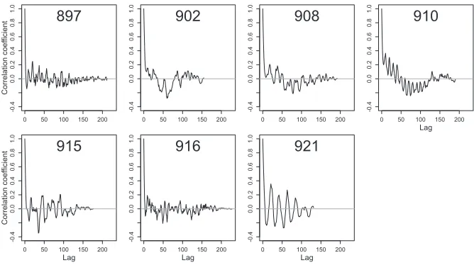
Telemetry data commonly feature high spatial and temporal autocorrelation. This can be present in locations, aspects of behavior or properties of the movement trajec-tory, and environmental variables collected in association with locations. The dive record of each individual was checked for spatial and temporal autocorrelation in maximum depth of consecutive dives using the autocorrelation function (ACF) (acf function, base package, R Development Core Team 2010). Gray seals do not dive at a constant rate (number of dives per unit time), so to view the autocorrelation in a more standardized temporal context, ACF plots of the raw data were constructed for the daily mean maximum dive depth of each individual (Fig. 1). The pattern of auto-correlation was not modeled; instead, it was dealt with by subsampling the data set. Taking every tenth dive from the track of each individual reduced the autocorrelation substantially. The resulting data set consisted of 21,986 dives from all trips from seven individuals (Fig. 2).
Statistical Modeling
A GAMM was fitted to the maximum dive depth time-series to generate spatial predictions of maximum dive depth. Individual was included as a random effect, to
0 50 100 150 200
-0.4
0.0
0.2
0.4
0.6
0.8
1.0
Correlation coef
ficient
897
0 50 100 150 200
-0.4
0.0
0.2
0.4
0.6
0.8
1.0
902
0 50 100 150 200
-0.4
0.0
0.2
0.4
0.6
0.8
1.0
908
0 50 100 150 200
-0.4
0.0
0.2
0.4
0.6
0.8
1.0
Lag
910
0 50 100 150 200
-0.4
0.0
0.2
0.4
0.6
0.8
1.0
Correlation coef
ficient
Lag
915
0 50 100 150 200
-0.4
0.0
0.2
0.4
0.6
0.8
1.0
Lag
916
0 50 100 150 200
-0.4
0.0
0.2
0.4
0.6
0.8
1.0
Lag
[image:5.495.84.418.414.601.2]921
Figure 1. The autocorrelation function (ACF) of the daily mean in maximum dive depth
capture the individual-level variability in dive depth. The explanatory variables included in the model were selected from the available variables on the premise that they characterize some aspects of the spatial, physical, and temporal environment that seals experience while at sea (bathymetry, horizontal displacement, latitude and lon-gitude, Julian day, sediment composition, light conditions), and individual charac-teristics of the tagged animals (individual identity). Sex and morphometrics were not used as explanatory variables. Knowledge of the diet of this population is incomplete and distribution data on known prey species is sparse. Instead, the percentage of gravel in the sediment was used as a proxy for the potential presence of sand eels, which are known to form a substantial part of seal diet on the east coast of the UK and western North Atlantic from scat sample analysis (Prime and Hammond 1990; Bowen and Harrison 1994; Hammondet al. 1994a,b). The variables used to explain maximum dive depth in the final model were bathymetry (range –4.0–200.9 m, source: DigBath250 data set, scale 1:250 000, British Geological Society), longitude in WGS84 decimal degrees (range 3.04–9.10), latitude in WGS84 decimal degrees (range 54.7–59.0), rate of horizontal displacement between surface locations (range 0.00–2.20 m/s), Julian day (range 100–334), percentage gravel in the sediment (range 0.00–83.0), and a binary variable for light conditions (daylight/darkness). A variable for “individual” was included as a random effect, with the assumption that the sample of individual seals, albeit small, is representative of the variability in max-imum dive depth characteristics of this population, and that their behavior is not more similar than would be expected by chance. Although the dives in this data set
come from just seven individuals, there was no reason to expect their diving behavior to be correlated.
Longitude, latitude, horizontal displacement rate, Julian day, and light conditions were taken directly from the data delivered by the tag or derived from them. Light conditions at the time of the dive were calculated as a binary variable (light or dark), based on the timing of each dive relative to local sunrise and sunset, using the sunri-set function in the maptools library (Lewin-Koh and Bivand 2011) in R.
The bathymetry and sediment data were processed as per Aarts et al. (2008), resulting in values on a 1 km grid for both variables. Bathymetry and sediment type were matched to dive locations using bilinear weights to interpolate values on a rect-angular grid to irregular locations, so that interpolated values at dive locations were interpolated along the x and y axes (latitude and longitude) from the four nearest points in the grid of bathymetry and sediment values. This was carried out using the interp.surface function in the fields package (Furreret al.2011) in R.
The nonlinear relationships between the response and many of the explanatory variables, and the potential for systematic variation in model residuals for dives made by the same animal, were accounted for by fitting a GAMM. Although the structure of the response data was such that there were two levels of nesting, dives from trips within individuals, a single random effect was included for individual, because the depth characteristics of dives from different trips within and between individuals were found to vary little.
The GAMM was implemented with the gam function in the mgcv library (Wood 2006, 2008) in R using fast restricted maximum likelihood (fREML) as the fitting method. The random effect for individual was implemented using the “re” smoother option, which is appropriate for simple, independent random effects (Wood 2011). Under this formulation random effects are implemented by applying a penalty to the model matrix in the form of a scalar multiple of the identity matrix, hence assuming that the coefficients associated with the penalty are inde-pendent and normally distributed (Wood 2008). The “gamma” parameter of the gam function (effectively a roughness penalty) was set to 1.4 (Wood 2006), to reduce the chance of over-fitting to the data. Latitude and longitude entered the model as a spherical smooth function of the response using the “sos” two-dimen-sional isotropic smoother option in the mgcv library, with a first derivative penalty, which is the default, and 100 knots. All other continuous variables were fitted as smoothed functions with a minimum of 6 (k=6) and a maximum of 10 knots (k =10) and daylight/darkness entered the model as a factor. The appropriate number of knots in each case was chosen using the routines outlined in the mgcv package manual and Wood (2006). Cubic regression splines (“cs”; this type of smooth incor-porates a smooth modification technique called shrinkage, which is discussed below) were used as the basis functions for all continuous variables.
estimation of confidence intervals (Wood 2006). A model with a Normal error distri-bution and an identity link function was used.
Variable Selection
A generalized additive model describes the response data as a smooth, nonlinear function of the covariates. To prevent over-fitting, any excessive “wiggliness” in the fitted model must be penalized. A strict penalization of the response to any given co-variate can shrink (i.e.,lessen) its effect without removing it from the model. Shrink-age smoothing methods allow smooth components to be shrunk to zero during smoothness selection, effectively extinguishing their effect from the model (Wood 2008). The appeal of shrinkage approaches is that (1) they have the consistency of methods that explore the combination of all possible subsets of covariates (subset selection); (2) with them, variable selection can be achieved in a single step; and (3) they explore a larger part of model space than stepwise model selection procedures because they do not remove (or include) a variable permanently and hence they always give the opportunity to all the variables to increase (as well as decrease) their contri-bution to the model. As a result, shrinkage approaches do not suffer from the uncer-tainty inherent in stepwise variable selection procedures and model subset selection (Marra and Wood 2011).
The mgcv library offers two methods for the modification of smooths that employ a shrinkage approach: “double penalty” and “shrinkage.” The double penalty approach was used because of its stability in prediction, and the advantage of being able to use it with any spline basis, including spherical splines. Despite it requiring twice the number of smoothing parameters to be estimated (Marra and Wood 2011), model fitting with the double penalty approach was still quick (approximately 2 min) on a machine with two 2.8 GHz quad-core Intel Xeon processors and 8 GB of RAM.
If penalization is strong enough, shrinkage smoothers will push all the coefficients of the smooth to zero, cancelling out its effect (Wood 2008). Hence, with increasing shrinkage, a model that contains the (shrunk) covariate tends to become equivalent to a model that does not.
Predictions
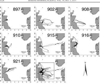
Julian day was set to 160 (8 June 2008), horizontal displacement to 0.3 m/s, which was the median value in the data. Predictions were made for each individual animal over a region containing the majority of track data (Fig. 2; longitudinal range 3.1º– 4.0º, latitudinal range 54.5º–59.1º), scaling each prediction matrix by the propor-tional contribution of each individual to the data set, in terms of number of dives. The seven scaled prediction matrices were then summed to produce population-level prediction maps, as described above.
Results
There was a persistent cyclic autocorrelation pattern in the raw data for all individuals, with successive increases and decreases in similarity between dive depths with increasing time lag. Some individuals reliably returned to the same areas and by similar routes during different trips (e.g., 897, Fig. 2) while others interspersed trips to regularly used areas, with long trips to distant or different areas (e.g., 915, Fig. 2). On the whole, all individuals used a small number of geographic regions frequently, with some overlap between individuals. There was little evidence for similarity or synchronicity in the pattern of autocorrelation present in the time series of depths from different individuals based on spectral density analysis of the dominant frequency of autocorrelation. This pattern was less pronounced in the thinned raw data, and there was no serial pattern in the model residuals.
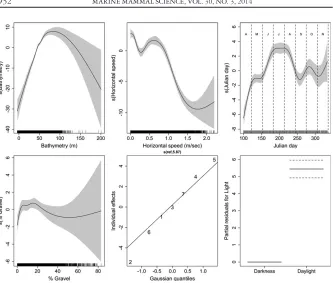
The plots of the component smooth functions (Fig. 3) show the overall relation-ship between maximum dive depth and each of the covariates, under the model. Max-imum dive depth had a clear, positive relationship with bathymetry until approximately 60 m. The negative relationship apparent at the upper end of the bathymetric range is largely unsupported by the data, which are concentrated in the range 0–100 m. The smooth for horizontal displacement (speed) suggests that ani-mals dive less deeply as horizontal displacement increases. The relationship with Julian day was variable, with the greatest maximum dive depth being reached in July (ca. day 200).
There was a positive relationship between maximum dive depth and the percent-age of gravel in the sediment up to 20% and a negative relationship with large stan-dard errors, with increasing gravel content, thereafter. The plot for the random effect for individual shows that although five out of seven animals had similar maximum dive depth characteristics, under the model, two of these (902 and 915, a male and female) had more extreme effects than the rest. Overall, the size of the individual effect was relatively small compared to the fixed effects, judging by the range of the y-axis. The partial residual plot for light conditions shows that the predicted maxi-mum depth for dives made in daylight was deeper than for those made during the hours of darkness.
The model captured 37% of the variability (model deviance) in the data. The dis-tribution of the residuals was, on the whole, symmetrical and centered on zero and there was no evidence for autocorrelation. There was some evidence of over-prediction in a small peak of negative residuals, which was also obvious in plots of observedvs. fitted values of maximum dive depth.
during the deployment period (two males, 902 and 908, and the largest of the four females, 915, Fig. 2) was Dogger Bank, to the southeast of Abertay Sands, at approximately 55ºN, 2ºW, where the model predicted that all three seals dived to the seabed. Two females (897 and 910, Fig. 2) used an area approximately 100 km west/northwest of Abertay Sands, and were also predicted to dive to the seabed (Fig. 4).
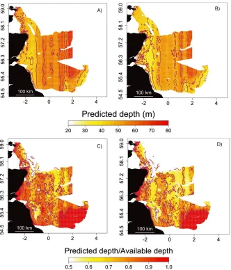
[image:10.495.79.412.61.344.2]The spatial predictions of maximum dive depth show a vertical band spanning the latitudinal range of the tracks, in which all seals appear to dive deeper both in light and dark conditions (Fig. 4A, B). Overall, dives made during darkness were predicted to be shallower across the whole area (Fig. 4B). The pattern of propor-tional use of the maximum available depth showed consistent predictions of diving to 70%–100% (0.7–1.0) of the available depth during daylight (Fig. 4C). When diving during darkness, animals utilized proportionally less of the available depth and dives were also shallower in absolute terms (Fig. 4D). This pattern varied spatially. Maximum dive depth was predicted to exceed 80% of the available depth only 25% of the time during darkness, compared to 46% during daylight. It would seem that these predictions indicate a shift to mid-water dives (60%–80% of available depth) during darkness (57% vs. 44% during daylight). Seals were also
predicted to spend more time in the upper part of the water column (less than 60% of available depth) during darkness (18% vs. 10% during daylight). There were some areas where there was no change in absolute maximum dive depth or proportional dive depth, the most distinct of which was the Dogger Bank.
Discussion
Spatial predictions of marine mammal distribution and habitat preference are most commonly presented in two dimensions, latitude and longitude. For diving animals, this is an inadequate representation of their use of space. We constructed a regression model to explain the conditions under which gray seals in the western North Sea dive to different maximum depths, based on a thinned data set of 21,986 dives from seven individuals that were instrumented with GPS phone tags on the east coast of the UK in April 2008. The model explained 37% of the variability in the response data over-all, and predictions were poor at the extremes of the observed range of the response variable, particularly when shallow dives were performed over deep water.
Descriptive metrics of diving, foraging behavior, and movement characteristics are often used in place of raw data (e.g., Schreer and Testa 1996, Fauchald and Tveraa 2003). These can be hard to interpret biologically without independent verification of function or their suitability as proxies for what they are intended to convey. The motivation for using maximum dive depth as the response variable was to investigate the usefulness of this very simple aspect of depth use in a benthic diver, for describing the relationship between diving behavior, environmental, spatiotemporal and indi-vidual covariates.
Given the strong association between sand eels, a primary prey type for benthic foragers such as gray seals and diving seabirds, and coarse sand and fine to medium gravel (Wrightet al.1998, van der Kooijet al.2008), sediment type could be con-sidered as a proxy for the availability of prey resources to species like gray seals, that feed on benthic or demersal prey (Wanless et al.1993, Gremillet et al. 1998, McConnell et al. 1999, Aarts et al. 2008, Watanuki et al. 2008). However, sand eels are not benthic divers’ only prey. The gray seals in this data set used primarily three water masses, as defined by Ehrlich et al. (2009): Scottish Coastal Water, North Atlantic Water, and Northern North Sea Water. Prey types represented in scat samples from the east coast of Scotland are probably only representative of prey taken by seals in Scottish Coastal Water. Trawls carried out in North Atlantic and Northern North Sea Water found that two gadids, haddock (Melanogrammus aeglefi-nus) and whiting (Merlangius merlangus) dominated their catches (Ehrlich et al. 2009). Although this cannot be used as evidence that gray seals consume these spe-cies, haddock and whiting also prey on sand eels and other species consumed by gray seals. Whiting in particular has been found to make up a large proportion of diet by weight late in the year based on scat sample analysis from Orkney (Ham-mondet al.1994a).
In this analysis, autocorrelation was dealt with by subsampling, resulting in loss of information about the time-series of dive depths immediately prior to a dive. It has been shown that gray seal diving behavior occurs in bouts and that there are different types of dive bouts (Becket al.2003c, Austinet al.2006). The temporal scale consid-ered in this analysis was that of individual dives and trips, but not the structure of dives within trips. It is likely that explicitly modeling the bout structure of seal div-ing behavior would lead to improved predictive power. Another temporal effect that might have contributed to dive depths being over-predicted at shallow depths might be the trip classification routine adopted here. The 3 h haul-out definition used to separate trips is likely to have excluded short trips in the vicinity of the haul-out, during which opportunistic foraging should not be ruled out. The individual whose dives were also most accurately predicted by the model, was the one that carried out the most trips in this study and whose dive depth at shallow depths was best repre-sented (897, see Fig. 2).
External features of the physical environment both in space and time (light/dark conditions, bathymetry, season, geographic coordinates) are considered to be ade-quately represented in the model, although tidal effects and currents, water tempera-ture, and stratification were not included and could have also explained some of the variability. Individual, internal factors that were not considered here and have been shown to affect diving behavior in gray seals include hormonal and metabolic status of the individuals, body mass, body condition, and the associated locomotory impli-cations (buoyancy) (Becket al.2000, 2003a, b, c).
These poorly predicted shallow dives made over deep water could be resting or digesting dives, since it has been documented for gray seals in captivity that food pro-cessing can be delayed for many hours after a feeding event (Sparlinget al.2007).
The negative effect of darkness on dive depth found here could be the result of the model inaccurately predicting a unimodal mean for bimodal night time diving behavior. If deep feeding dives are interspersed by shallow processing or resting dives, the effect could be an intermediate predicted dive depth. Alternatively, if seals feed at or just above the seabed during the day, the positive effect of daylight on dive depth ties in with the diurnal behavior of sand eels, which feed in the water column in the day and bury themselves in the sediment at night (van der Kooijet al.2008), though there is anecdotal evidence that they can also spend time buried during daylight hours. It is possible that when targeting sand eels or other vertically migrating prey, gray seals dive deeper in the day and spend the hours of darkness carrying out shal-lower dives during which other metabolic functions can be carried out, or even feed-ing on other prey.
investigated here, but given the diurnal effect on dive depth, dive duration may fol-low a similar pattern.
To summarize, the effect of environmental, behavioral, and individual character-istics on maximum dive depth was investigated using a data set of trips from seven animals. A small number of covariates explained a non-negligible proportion of the variability in the data, even though no intrinsic variables were considered. Although, by design, this analysis does not examine the causal relationship behind dive depth, i.e., the mechanism that drives the alternation between shallow and deep dives, we show that this aspect of vertical space use in the marine environment can be described and predicted with commonly available data on spatiotemporal co-variates. This is useful as a baseline for understanding depth use using regression models, and could be used as the first step in a two-part regression model for depth use, for explaining distribution of depths, given the maximum depth visited. Depth aside, longer dives might suggest more profitable, higher quality patches in the wild as has been found in captivity (Sparling et al. 2007), which could be investi-gated further.
The variability in the effect of the spatial and temporal covariates (bathymetry, Julian day, light conditions, gravel) suggests that foraging effort is spatially and tem-porally heterogeneous between individuals. However, the scale of the vertical axis of the smooth functions for the fixed effects, particularly bathymetry, horizontal speed, and Julian day, relative to the random effect suggests that the effect of individual var-iability captured by this covariate is relatively small compared to environmental effects.
With this analysis of gray seal diving we illustrate the use of a mainstream sta-tistical method, a GAMM, to generate three-dimensional maps of dive depth in marine animals. These maps of spatial predictions of maximum dive depth, an aspect of depth use, contribute to knowledge of diving species’ biology, and make it possible to estimate and visualize the potential rate of interaction between diving animals and subsurface developments, such as marine renewable energy installations (Furness et al. 2012). This approach is relevant to plunge and pursuit diving sea-birds (e.g., gannets, Sula spp., and cormorants, Phalacrocorax spp.), pinnipeds, and cetaceans that focus the effort at the deepest part of their dives. Usage maps based on spatial predictions of the distribution of maximum dive depth can be generated in this way for large areas, provided dive data and environmental data are available. An integration of two-dimensional maps of habitat use and maps of dive depth would provide a more complete view of diving animals’ space use and movement ecology.
Acknowledgments
Literature Cited
Aarts, G., M. Mackenzie, B. McConnell, M. Fedak and J. Matthiopoulos. 2008. Estimating space-use and habitat preference from wildlife telemetry data. Ecography 31:140–160.
Austin, D., W. D. Bowen, J. I. McMillan and S. J. Iverson. 2006. Linking movement, diving, and habitat to foraging success in a large marine predator. Ecology 87:3095– 3108.
Beck, C. A., W. D. Bowen and S. J. Iverson. 2000. Seasonal changes in buoyancy and diving behavior of adult gray seals. Journal of Experimental Biology 203:2323–2330.
Beck, C. A., W. D. Bowen, J. I. McMillan and S. J. Iverson. 2003a. Sex differences in the diving behavior of a size dimorphic capital breeder: The gray seal. Animal Behavior 66:777–789.
Beck, C. A., W. D. Bowen and S. J. Iverson. 2003b. Sex differences in the seasonal patterns of energy storage and expenditure in a phocid seal. Journal of Animal Ecology 72:280–291. Beck, C. A., W. D. Bowen, J. I. McMillan and S. J. Iverson. 2003c. Sex differences in diving at multiple temporal scales in a size-dimorphic capital breeder. Journal of Animal Ecology 72:979–993.
Beck, C. A., S. J. Iverson, W. D. Bowen and W. Blanchard. 2007. Sex differences in gray seal diet reflect seasonal variation in foraging behavior and reproductive expenditure: Evidence from quantitative fatty acid signature analysis. Journal of Animal Ecology 76:490–502.
Bowen, D. W., and G. D. Harrison. 1994. Offshore diet of gray sealsHalichoerus grypusnear Sable Island, Canada. Marine Ecology Progress Series 112:1–11.
Bowen, D. W., J. W. Lawson and B. Beck. 1993. Seasonal and geographic variation in the species composition and size of prey consumed by grey seals (Halichoerus grypus) on the Scotian Shelf. Canadian Journal of Fisheries and Aquatic Sciences 50:1768–1778. British Geological Society. DigBath250. [Data set]. Available at http://www.bgs.ac.uk/
products/digBath250/home.html.
Ehrlich, S., V. Stelzenm€uller and S. Alderstein. 2009. Linking spatial pattern of bottom fish assemblages with water masses in the North Sea. Fisheries Oceanography 18:36–50. Fauchald, P., and T. Tveraa. 2003. Using first-passage time in the analysis of area-restricted
search and habitat selection. Ecology 84:282–288.
Fedak, M. A., S. S. Anderson and M. G. Curry. 1983. Attachment of a radio tag to the fur of seals. Journal of Zoology 200:298–300.
Fedak, M. A., P. Lovell and B. J. McConnell. 1996. MAMVIS: A marine mammal behavior visualization system. Journal of Visualization and Computer Animation 7:141–147. Furness, R. W., H. M. Wade, A. M. C. Robbins and E. A. Masden. 2012. Assessing the
sensitivity of seabird populations to adverse effects from tidal stream turbines and wave energy devices. ICES Journal of Marine Science 69:1466–1479.
Furrer, R., D. Nychka and S. Sain. 2011. fields: Tools for spatial data. R package version 6.6. Available at http://CRAN.R-project.org/package=fields.
Google, Inc. 2009. Google Earth (Version 3.0.11733). Available at http://www.google.com/ earth/index.html.
Gremillet, D., G. Argentin, B. Schulte and B. M. Culik. 1998. Flexible foraging techniques in breeding cormorantsPhalacrocorax carboand ShagsPhalacrocorax aristotelis: Benthic or pelagic feeding? Ibis 140:113–119.
Hammond, P. S., A. J. Hall and J. H. Prime. 1994a. The diet of gray seals around Orkney and other island and mainland sites in north-eastern Scotland. Journal of Applied Ecology 31:340–350.
Hammond, P. S., A. J. Hall and J. H. Prime. 1994b. The diet of gray seals in the Inner and Outer Hebrides. Journal of Applied Ecology 31:737–746.
Kooyman, G. L., and P. J. Ponganis. 1998. The physiological basis of diving to depth: Birds and mammals. Annual Review of Physiology 60:19–32.
Marra, G., and S. N. Wood. 2011. Practical variable selection for generalized additive models. Computational Statistics and Data Analysis 55:2372–2387.
McConnell, B. J., M. A. Fedak, P. Lovell and P. S. Hammond. 1999. Movements and foraging areas of gray seals in the North Sea. Journal of Applied Ecology 36:573–590.
Meir, J. U., C. D. Champagne, D. P. Costa, C. L. Williams and P. J. Ponganis. 2009. Extreme hypoxemic tolerance and blood oxygen depletion in diving elephant seals. American Journal of Physiology Regulatory, Integrative and Comparative Physiology 297:927– 939.
Lewin-Koh, N. J., R. Bivand, contributions by E. J. Pebesma, E. Archer, A. Baddeley,et al. 2011. maptools: Tools for reading and handling spatial objects. R package version 0.8-10. Available at http://CRAN.R-project.org/package=maptools.
Prime, J. H., and P. S. Hammond. 1990. The diet of gray seals from the south-western North Sea assessed from analyses of hard parts found in faeces. The Journal of Applied Ecology 27:435–447.
R Development Core Team. 2010. R: A language and environment for statistical computing. R Foundation for Statistical Computing, Vienna, Austria.
Schreer, J. F., and J. W. Testa. 1996. Classification of Weddell seal diving behavior. Marine Mammal Science 12:227–250.
Sparling, C. E., and M. A. Fedak. 2004. Metabolic rates of captive gray seals during voluntary diving. The Journal of Experimental Biology 207:1615–1624.
Sparling, C. E., M. A. Fedak and D. Thompson. 2007. Eat now, pay later? Evidence of deferred food-processing costs in diving seals. Biology Letters 3:94–98.
Thompson, D., P. S. Hammond, K. S. Nicholas and M. A. Fedak. 1991. Movements, diving and foraging behavior of gray seals (Halichoerus grypus). Journal of Zoology 224:223–232. van der Kooij, J., B. E. Scott and S. Mackinson. 2008. The effects of environmental factors on daytime sandeel distribution and abundance on the Dogger Bank. Journal of Sea Research 60:201–209.
Wanless, S., T. Corfield, M. P. Harris, S. T. Buckland and J. A. Morris. 1993. Diving behavior of the shag Phalacrocorax aristotelis(Aves: Pelecaniformes) in relation to water depth and prey size. Journal of Zoology 231:11–25.
Watanuki, Y., F. Daunt, A. Takahashi, M. Newell, S. Wanless, K. Sato and N. Miyazaki. 2008. Microhabitat use and prey capture of a bottom-feeding top predator, the European shag, shown by camera loggers. Marine Ecology Progress Series 356:283–293.
Wood, S. N. 2006. Generalized additive models: An introduction with R. CRC Press, Boca Raton, FL.
Wood, S. N. 2008. Fast stable direct fitting and smoothness selection for generalized additive models. Journal of the Royal Statistical Society B 70:495–518.
Wood, S. N. 2011. Fast stable restricted maximum likelihood and marginal likelihood estimation of semiparametric generalized linear models. Journal of the Royal Statistical Society B 73:3–36.
Wright, P. J., S. S. Pedersen, C. Anderson, P. Lewy and R. Proctor. 1998. The influence of physical factors on the distribution of lesser sand eels, Ammodytes marinus, and its relevance to fishing pressure in the North Sea. ICES Document CM 1998/AA: 03. 18 pp.