Measurements on cortical human, cortical bovine and simulated cortical bone

(1)

BACHELOR THESIS

MEASUREMENTS ON

CORTICAL HUMAN,

CORTICAL BOVINE AND

SIMULATED CORTICAL

BONE.

Nander Alblas

FACULTY OF ENGINEERING TECHNOLOGY LABORATORY OF BIOMECHANICAL ENGINEERING

EXAMINATION COMMITTEE

Prof. dr. ir. G.J. Verkerke Ir. E.E.G. Hekman Dr. H.K. Hemmes

DOCUMENT NUMBER

BW - 443

(2)

1 | P a g e

Preface:

This report is written as a Bachelor Assignment at the University Twente. This Assignment is a part of research done on the effects of heat on human cortical bone, bovine cortical bone and simulated cortical bone. This assignment is executed on behalf of ir. Hekman of the chair of Biomechanical Engineering at the University Twente.

(3)

2 | P a g e

Abstract:

In order to accurately model the effects of medullary reaming, accurate values of the thermal properties and density of human cortical bone are required. Since bovine bones and artificial bone substitutes made from epoxy filled with short glass fibers are often used when human bones are not available these materials have to be tested as well. This paper discusses the various methods that can be used to determine these properties, the use of the transient plane source method and a gas pycnometer in order to determine these properties and the eventual results from these

(5)

4 | P a g e

List of figures

Figure 1. One-Dimensional heat conduction... 9

Figure 2. Schematic overview of the comparative cut bar test. ... 11

Figure 3. Schematic overview of the guarded heat flow meter method. ... 12

Figure 4. Schematic overview of the guarded hot plate method. ... 13

Figure 5. Schematic overview of the transient plane source method. ... 13

Figure 6. Schematic overview of the transient hot strip method. ... 14

Figure 7. Schematic overview of the Pulse Transient Method and an example of the temperature response. ... 14

Figure 8. Transient recording of the thermal transport properties of the material surrounding the sensor. ... 15

Figure 9. Sensor and sample temperature increase curves. ... 16

Figure 10. Various RTD sensors. ... 21

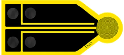
Figure 11. Kapton sensor. ... 23

Figure 12. Sample support and a LEMO connector with a kapton sensor attached. ... 24

Figure 13. Hot Disk TPS 2500S Thermal Constants Analyser. ... 24

Figure 14. AccuPyc II 1340 Density Analyzer. ... 25

Figure 15. Example of a drift graph. Temperature drift vs. Time. ... 28

Figure 16. Example of a transient graph. Temperature increase vs. Time... 29

Figure 17. Best fit line. Temperature vs. D(τ) ... 29

Figure 18. Residual plot. Temperature difference vs. the square root of the time. ... 29

Figure 19. Example of a boxplot using the interquartile ranges method. ... 30

Figure 20. Boxplot of the thermal conductivity of the epoxy samples containing the overall average, the mean, the highest/lowest values and the inner fence upper/lower limits. ... 33

Figure 21. Boxplot of the thermal conductivity of the bovine samples containing the overall average, the mean, the highest/lowest values and the inner fence upper/lower limits. ... 34

Figure 22. Boxplot of the thermal conductivity of the human samples containing the overall average, the mean, the highest/lowest values and the inner fence upper/lower limits. ... 34

Figure 23. Boxplot of the density of the epoxy, bovine and human samples containing the mean, the highest/lowest values and the inner fence upper/lower limits. ... 35

Figure 24. The thermal conductivities (W/m K) of the epoxy samples, the bovine samples, human samples and their averages in the longitudinal direction (L), radial direction (R) and transversal direction (T) ... 38

Figure 25. The thermal conductivities (W/m K) of the bovine samples in the longitudinal direction (L), radial direction (R) and transversal direction (T). ... 39

(6)

5 | P a g e

List of tabels

Table 1. Bone sample properties... 25

Table 2. Calculated examples. Measurements of the radial epoxy samples 1-3. ... 31

Table 3. Calculated examples. Measurements of the radial epoxy samples 1-3 with fixed volumetric specific heat. ... 31

Table 4. PMMA measurements. ... 32

Table 5. Volumetric Specific Heat. ... 32

Table 6. Thermal conductivities with various specific heats calculated using a radial measurement on an epoxy sample. ... 32

Table 7. Thermal conductivities. ... 33

Table 8. Average density. ... 35

Table 9. measurements of the thermal conductivity of cortical bone. ... 37

List of appendixes

Appendix A. Results of the thermal conductivity measurements. Appendix B. PMMA test results from Hotdisk.

Appendix C. Results of the density measurements. Appendix D. Gas pycnometer specifications.

(7)

6 | P a g e

(8)

7 | P a g e

1.1 Introduction:

Broken bones, when the fracture is severe enough, are often fixated using titanium pins and screws. Small holes are drilled and screws are inserted to which the pins are attached. When the fracture is healed the pins and screws are removed and the bone can continue to heal. In more invasive

situations, when a long bone can’t be fixated from the outside or when a hip joint has to be replaced, metal pins have to be inserted into the medullary cavity. To make the pins fit, excess bone has to be removed. This is called reaming. During the reaming of these bones heat is generated. This

generation of heat is a common problem when mechanized cutting tools are used for surgical preparation. When the temperature of the bone is raised above a certain threshold for a certain amount of time, thermal necrosis will ensue. This type of surgical trauma can lead to impaired bone healing. This impaired healing can be an issue when trying to fixate an implant for a hip replacement. If enough thermal necrosis has occurred the implant will be surrounded by connective tissue, instead of being firmly anchored in the living bone [12, 15]. Different methods are being used and tried out to reduce the heat generation or increase the heat dissipation. Drill speed, the applied force and the feed rate can be varied and the geometry of the drill can be changed to find a combination which produces the least amount of heat. Another option is to apply a coolant to the surface of the drill. To find out which variations and methods are the most successful the temperature increase inside the bone has to be measured. The measurement of these temperatures can be difficult. An often used method is the placement of thermocouples in the tissue surrounding the drill site. The accuracy of this method can be improved by placing more thermocouples. This is a labor intensive process and is impractical when multiple methods have to be tested. A quick way to test and predict the outcome of a specific combination of drill speed, drill geometry, etc, would be to model it. In order to model the situation, accurate measurements of the properties of the bone have to be known. More specifically; the thermal conductivity, specific heat and volumetric mass density of cortical bone. All three of these characteristics have been determined in various ways in the past. However, the thermal conductivities of cortical human and bovine bone found in these experiments vary greatly [12]. So the goal of this assignment is to find an easy and quick way to determine these three characteristics of different samples of different sizes and different origins.

1.2 Background information:

1.2.1 Thermal conductivity of bone

Thermal conductivity is a material property that corresponds to the rate at which the material can transfer heat. It is defined as:

where Q is the amount of heat passing through the cross section A , causing a temperature difference ΔT over a distance ΔL. Q/A is defined as the heat flux, which causes a thermal gradient

ΔT/ΔL. There are two classes of methods for the measurement of thermal conductivity: the steady-state method and the non-steady-steady-state (or transient) method. In both methods the entire heat flux must be uniaxial. Heat losses or gains must be minimized in the radial direction. At lower

(9)

8 | P a g e

It is also thought that bone is, to some extent, anisotropic. This might have an influence on its

thermal conductivity. This is why all samples will be tested in three directions; longitudinal, radial and circumferential.

1.2.2 Heat capacity of bone

The heat capacity is a physical quantity that specifies the amount of heat energy required to change the temperature of an object by a given amount. Here, we are interested in the specific heat capacity. This is the heat capacity per unit mass of the material. The best known method of

determining the heat capacity of a material is calorimetry. In this method a known amount of heat is added to the material. The temperature before and after the heating process is observed and from this observation one can calculate the heat capacity using:

( )

In which q is the amount of heat added, C the heat capacity, the systems final temperature and the systems initial temperature. To obtain the specific heat one has to divide the heat capacity by the mass of the system.

Another option is available when using a transient measuring method. Using the transient method one has to fit experimentally found data to a theoretical model. With a proper fit one can then determine the thermal conductivity and the thermal diffusivity, a materials ability to conduct thermal energy relative to its ability to store thermal energy. The specific heat of the material can then be calculated using:

(10)

9 | P a g e

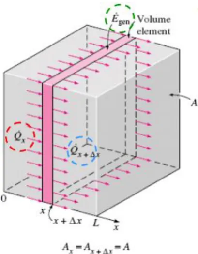
[image:10.595.198.403.99.362.2]

1.2.3 The Heat Conduction Equation, 1D Heat Flow.

Figure 1. One-Dimensional heat conduction.

To determine the temperature profile of the sample while heating we need the differential equation of heat conduction. Most of the steady-state setups are build to only allow heat flow in one

direction, so you can simplify the equation to a single dimension.

The total rate of heat generation in a medium of volume V and the heat generated by a heating element consisting of a wire coil can be determined from:

∫ and

In one dimension the heat conduction equation consists of:

In which is the rate of heat conduction at x, is the rate of heat conduction at x+ ,

is the rate of heat generation inside the element and is the rate of change of

the energy content of the element.

and can be rewritten to:

This can be substituted into the previous equation. Dividing by , taking the limit as and

and applying Fourier’s law we are left with:

(

)

(11)

10 | P a g e

When assuming the area A stays constant, the one dimensional transient heat conduction equation becomes:

(

)

For the steady-state heat conduction equation one simply has to equate ( ) .

When also assuming that the conductivity is constant in the sample one can simplify the equation further to:

⁄

1.2.4 Steady-State Measurement Methods

Generally, when using a steady-state method, the temperature of the measured material does not change with time. . In the steady-state method the measurement of the heat flux can be done directly or indirectly. It can be done directly, for example, by measuring the electrical power used by the heating element that is used to heat the sample. Or it can be done indirectly by using a

comparative method in which the thermal gradients of a known and unknown sample are compared.

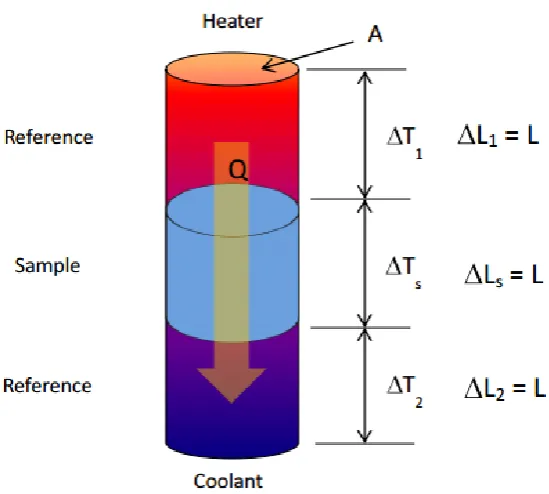
Axial Flow Methods.

This method is usually a cylindrical setup in which a heater transfers heat through the sample to a coolant. A know amount of power is send through a heating element after which the thermal conductivity can be calculated from the temperature gradient between the two ends of the sample. Axial Flow methods are known for their high accuracy and consistency and are usually the method of choice at cryogenic temperatures. The main issue with this method is the reduction of radial heat loss of the specimen. At higher temperatures this becomes more difficult [1].

Comparative cut bar (ASTM E1225)

(12)

[image:12.595.164.439.82.329.2]

11 | P a g e

Figure 2. Schematic overview of the comparative cut bar test.

The thermal conductivity of the sample ( can be derived from the thermal conductivity of the reference ( ).

[1].

Guarded and unguarded heat flow meter methods (ASTM C518, ASTM E1530)

This method requires the use of a flux gauge, or heat flux sensor. A heat flux sensor is usually a very thin piece of reference material with a low thermal conductivity containing a large number of thermocouple pairs. The heat passing through the flux gauge (Q) can be derived from the thermal conductivity of the reference ( ), the temperatures on either side of the sensor ( and ) and the thickness of the resistive layer.

(13)

[image:13.595.175.429.69.262.2]

12 | P a g e

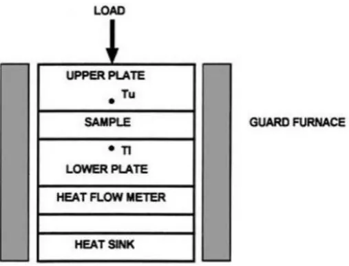
Figure 3. Schematic overview of the guarded heat flow meter method.

Figure 2 shows a setup for a guarded heat flow meter. A small sample is held under a compressive load between two plates that both contain thermocouples. A heat flux gauge is placed below the lower plate. Guards make sure no heat is lost to its surroundings. Guards can be active or inactive. Inactive guards consist of isolating materials. Active guards, also known as guard heaters, contain thermocouples and a heat source. Guard heaters are used to insure that the guard temperature is as close as possible to the temperature of the outer wall of the setup. An axial temperature gradient is established across the upper plate, sample and lower plate. The thermal conductivity can be determined by using this thermal gradient and the output of the flux gauge. At thermal equilibrium the thermal resistance ‘ ’ is:

Where and are the temperatures of the upper and lower plate and Q is the heat flux gauge output. is the interfacial thermal resistance, also known as thermal boundary resistance. It is a

measure of an interface’s resistance to thermal flow [1].

Guarded Hot Plate Method (ASTM C177)

With this method two specimens are selected with their thickness, areas and densities as identical as possible. One specimen is placed on each side of the guarded hot plate. The side opposite to the side which is in contact with the hot plate of both samples is placed against a cold contact surface. Guards or guard heaters are used to keep the system adiabatic. When the system is in a steady-state, a constant heat flows through the specimens. The thermal conductivity is determined using this heat flow, the average temperature difference between the specimen surfaces and the size of the

specimen.

Both the heat flow meter methods and the guarded hot plate methods become inaccurate when there is free moisture inside the test sample. Free moisture inside the sample may cause transient behavior. Both methods also become less accurate when the used sample is

(14)

[image:14.595.153.441.71.218.2]

13 | P a g e

Figure 4. Schematic overview of the guarded hot plate method.

1.2.5 Transient Measurement Methods

Transient methods are related to the heat conduction equation, which relates the change in

temperature with time, . These methods are based on measuring the sample’s behavior in the transient regime of heat flow.

“Recently, it has been shown that a group of techniques known as Contact Transient Methods (CTM) should be suitable for this class of materials. In comparison with stationary or steady state methods the advantage of the transient methods is that some of them give a full set of thermophysical parameters within a single measurement, namely specific heat, thermal diffusivity, thermal conductivity or effusivity.” [10]

Transient Plane Source

In the Transient Plane Source technique, sometimes also called the Hot Disk Method, a thin double-spiral sensor is placed between two identical pieces of sample material. The sample material has to completely cover the sensor. Power is supplied to the sensor, resulting in step-wise heating. This results in a transient temperature response that is recorded by the same spiral. The double spiral gives a constant heating rate per unit spiral length and at the same time operates as a resistance thermometer. Using this setup one can consider the heat flow as 1D, has to regard the specimen as an infinite medium and measure the change in electrical resistance in the sensor because of the temperature increase. [10]

(15)

14 | P a g e

Transient Hot Strip/Wire

The Transient Hot Strip and Transient Hot Wire methods are based on the same principles as the Transient Plane Source method. A thin strip or wire of metal, capable of producing an essentially constant heating rate, is placed between two identical samples. The downside of this method is that it requires long samples since the sensitivity of a resistance thermometer is directly proportional to the initial resistance of the wire or strip. [10, 16]

Figure 6. Schematic overview of the transient hot strip method.

Pulse Transient Method

The Pulse Transient Method requires a setup as shown in figure 4. A heat pulse is generated by an electrical current through a plane electrical resistor. The temperature response is measured by a thermocouple. The thermal diffusivity, specific heat and thermal conductivity can be calculated from the parameters of the temperature response (figure 5).

Figure 7. Schematic overview of the Pulse Transient Method and an example of the temperature response.

Using:

√ ,

√

one can calculate the thermal diffusivity α, the specific heat c and the thermal conductivity k. h is the thickness of the specimen, is the time it takes to reach the maximum of the temperature

(16)

15 | P a g e

1.2.6 Transient Methods, Temperature and Resistance.

[image:16.595.82.526.167.259.2]

In the Hot Disk, Hot Strip and Pulse Transient methods a wire or strip is used as both a heat source and a resistance thermometer. When a precisely known amount of power is delivered to the wire or strip, the increase in temperature and thus the change of the resistance in the wire or strip, can be used to determine the thermal conductivity and thermal diffusivity of the samples.

Figure 8. Transient recording of the thermal transport properties of the material surrounding the sensor.

Because the sensitivity of a resistance thermometer is proportional to its initial resistance and thus its length, the resistance thermometer should be as long as possible. The Hot Disk sensor has been designed in the form of a double spiral to minimize the required sample size and to keep the sensor compact. If it is assumed that the Hot Disk consists of a certain number of concentric ring heat sources, located in an infinitely large sample, the thermal conductivity equation can be solved as following.

When electrically heated the resistance increases as a function of time:

{ [ ]}

Where is the resistance of the disk at time t = 0, is the Temperature Coefficient of the Resistivity, is the constant temperature difference that develops almost instantly over the thin insulating layers that cover the wire of the sensor and is the temperature increase of the

sample surface.

From the previous equation we get the temperature increase recorded by the sensor:

(

)

(17)

[image:17.595.161.438.78.283.2]

16 | P a g e

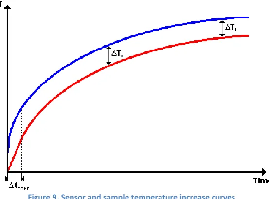
Figure 9. Sensor and sample temperature increase curves.

Figure 9 shows the temperature increase of the sensor itself (blue) and the temperature increase of the surface of the sample (red). After a short time the becomes constant. This time, , can be estimated as:

Where δ is the thickness of the insulating layer of the sensor and is the thermal diffusivity of the layer.

The time-dependent temperature increase is given as:

Where is the total power output from the sensor, is the overall radius of the disk, is the thermal conductivity of the sample and is a dimensionless time dependent function with:

√

Where is the time measured from the start of the recording and Θ is the characteristic time given by:

where is the thermal diffusivity of the sample.

When we make a computational plot of the recorded temperature increase versus , we obtain a straight line. When using experimental times significantly longer than the intercept of this line is

and its slope is

. Because and Θ are unknown before the experiment, the final line from

(18)

17 | P a g e

(19)

18 | P a g e

2.1 Problem analysis

The assignment contains the following goals;

- Determining suitable measuring methods for:

 Thermal conductivity

 Specific heat

 Density - Sample preparation

- The performing of said measurements - Process and interpret the data

As discussed earlier there are two main branches when measuring the thermal conductivity,

transient and steady-state. Both methods have multiple variations that each has its own advantages and disadvantages. From these advantages and disadvantages, in combination with any limitations that follow from the preparation of the samples or the samples themselves, a method has to be chosen.

The measurements will be performed on three types of samples;

- Epoxy which is filled with short glass fibers, a material that is currently being used as an artificial replacement for tests when real bone is not available

- Cortical bone from a bovine femur - Cortical bone from a human femur

The thickness of the cortical bone of a human femur lies between 1 and 10 mm [19]. The thickness of human cortical bone lies in the same range [20]. The thickness of the available simulated cortical bone varied between 5.5 and 6 mm. This is something that has to be kept in mind when choosing a design. The cortical bone, after it is prepared, has to be kept frozen or submerged in water in order to preserve the samples. In each of the measurement methods the sample is heated to a certain temperature. Keeping the bone samples at a certain temperature for a prolonged period of time might damage the sample or change its composition.

Another requirement that has to be taken into account is that the measurements have to be

(20)

19 | P a g e

2.2 Analysis of measuring methods

Steady-State conclusion:

“Steady-state heat transmission through thermal insulators is not easily measured, even at room temperature. This is because heat may be transmitted through a specimen by any or all of three separate modes of heat transfer (radiation, conduction, and convection); any inhomogeneity or anisotropy in the specimen may require special experimental precautions to measure that flow of heat; hours or even days may be required to achieve the thermal steady-state; no guarding system can be constructed to force the metered heat to pass only through the test area of insulation

specimen being measured; moisture content within the material may cause transient behaviour; and physical or chemical change in the material with time or environmental condition may permanently alter the specimen.”[7]

All these methods require the use of homogeneous and opaque solid samples and reference

materials. C117 and C518 also have problems with materials containing moisture and C117 is known to have a significant waiting period (hours or even days) for the system to get to a thermal steady-state. C518 requires calibration using method C117. With the for the C117 method required circumstances the error introduced by this calibration is around 2% [5]. Since we are working with human cortical bone, which is neither homogeneous nor moisture free, this error is expected to be larger.

In the paper “The effects of moisture on thermal conductivity of fibrous biological insulating materials” [8] Guru S Kochhar and K. Manohar tested the effects of moisture on biological material called ‘bagasse’, a fibrous material made from sugarcane. The difference in thermal conductivity between an air dried sample and sample which had 5% moisture added was around 17%. Since this difference is the result of free water enclosed in the material, the enclosed water inside cortical bone will most likely have a similar effect on the measurement. In skeletally mature cortical bone around 10% of its wet weight is water [9]. Also, due to a temperature difference that has to be maintained for a long period of time, a non-uniform moisture distribution may arise. This may lead to

conductivity measurements that depend on the sample size and the magnitude of the applied temperature difference [13].

E1225 is a simple variation of E1530, E1530 is a modification of C518 and C518 requires calibration which requires the use of method C117. Therefore it may be assumed that the general downsides like the requirement of homogeneous materials, the time required to achieve steady state and the presence of moisture are present in all discussed steady state methods and the methods which are small variations on the discussed methods [4],[5],[6],[7].

Transient method conclusion:

“The motive behind the development of the TPS technique has been to cover as large ranges of the transport properties as possible and at the same time be able to apply the technique to a large number of different materials.” [11]

When using a resistive element both as a heat source and a measuring device one can simply record the voltage change over the source/sensor while its temperature is heated by an electrical current pulse. One of the problems with plane sources, namely the requirement that the sample has to be considered as an infinite or semi-infinite medium, can be neglected by choosing a short enough current pulse. “This means that the time of a transient recording must be chosen so that the outer boundaries of the sample do not influence the temperature increase of the element to any

(21)

20 | P a g e

In the design of a Transient Plane Source element, 5 important points have to be taken in consideration:

- The current needed for the heating. - A constant driving voltage.

- The electrical sensitivity needed for the recordings with an average temperature increase not exceeding 1 Kelvin.

- The reduction of non-ohmic impedance to a minimum.

- The difference in heat capacity between the sample and the Transient Plane Source Element.

The current needed for the heating, the driving voltage and the measurement time have to be balanced to make sure that the heat generated does not reach the boundaries of the sample. As long as these boundaries are not reached an increase of the temperature gradient will increase the accuracy of the measurement.

“The impedance should ideally be strictly ohmic, particularly if a dc voltage is used for the heating element. Otherwise a certain finite rise time of the heating current at the start of the transient event will prevent the immediate output of power in the element” [11].

When using samples with a low heat capacity, one cannot neglect the effects of the heat capacity of the TPS on the measurement. Nickel is usually used as the resistive element in TPS methods. With the thermal conductivity of nickel being 90.9 W/(m*K) and the thermal conductivity of cortical bovine bone being around 0.55 W/(m*K) [12] this most likely has to be taken into consideration. This is not a big problem, since it can be mended by a small addition to the original equations [11].

Where steady-state methods have a major drawback when moisture is present in the sample, transient techniques are fast and therefore less likely to produce non-uniform moisture distribution [13].

Another possible advantage of the transient methods is the determination of the specific heat. With the transient methods both the thermal conductivity and the thermal diffusivity are determined. Using;

the specific heat can be determined as long as the thermal conductivity and thermal diffusivity are determined accurately.

In the paper “Measurement of building materials by transient methods” [10] the statistical errors calculated for transient techniques where always below 3%. The Statistical errors of average values evaluated in % for the in this text discussed transient methods are 5% for thermal diffusivity, 4% for specific heat and 3% for thermal conductivity [10].

Final conclusion:

(22)

21 | P a g e

2.3 Choice of Method

A transient method, as discussed in the previous chapters, is most likely the best option. In the branch of the transient measurements there are three main methods. The transient hot strip/wire method, the pulse transient method and the transient plane source method. In order to determine the best method and materials we have to look at the requirements and the limitations from the samples. One of the requirements is that the measurements can be performed in the longitudinal, radial and transversal directions. If each of these three methods is to be performed on the same sample the best option would be to prepare the samples as cubes. With the limitation on size; 5.5-6 mm for the simulated cortical bone samples and 1-10 mm for the cortical bovine and human bone samples, a method capable of performing the measurements on sample the size of 5x5x5 millimeter would be preferable. The transient hot strip/wire method requires long samples and is therefore an undesirable method. Both the pulse transient method and the transient plane source method can be used for cubic samples. But the transient plane source method requires less separate components, is easier to dismantle and rebuild. The transient plane source method is also used more often leading to a larger knowledge base of its performance and a better availability of components.

[image:22.595.141.454.377.571.2]

Transient plane source measurements can be done with sensors of different shapes and sizes. These sensors are called resistance thermometers or resistance temperature detectors (RTD’s). Although they have their differences, they function by the same principle. By applying a current their temperature increases which in turn increases their resistance.

Figure 10. Various RTD sensors.

From these sensors the kapton sensor is the best candidate. It is flexible, durable, easy to hook up to a measurement setup and provides excellent surface contact with the samples. The sensor can be attached to a multitude of programmable development platforms, but the optimal solution would be to attach it to a Hot Disk Thermal Constants Analyser. This system is specifically designed by Hot Disk to be used in combination with their kapton sensors. One of the requirements of the kapton sensor is that it requires an identical sample on each side of the sensor. This is a downside because you

require twice the amount of samples and an upside because this makes the measurement more accurate. This is because one sided sensors require or contain shielding on one side which can negatively influence the measurement if the shielding is improper.

(23)

22 | P a g e

(24)

23 | P a g e

3.1 Introduction

Contact has been made with Ko Schaap, one of the sales and application representatives of Benelux Scientific. Benelux Scientific is the main distributor of products from Hot Disk Instruments in the Benelux area. They offered the usage of their equipment in order to perform the tests. Namely, the Hot Disk TPS 2500 S Thermal Constants Analyser, the kapton sensor and other required accessories. With the help of Nico Verdonschot, Leon Driessen and Pawel Thomaszew at the UMC Radboud the bone samples were obtained and prepared. The gas pycnometer that is required for the density measurements is available on the University of Twente which can use under the supervision of Beata Koziara.

3.2 Required components

The following components are required for the chosen setup in order to measure the thermal conductivity and specific heat:

- A kapton sensor of the correct size

- A support structure in which the samples and sensor can be placed - A Hot Disk TPS 2500 system

- A connector between the sensor and system

For the measurement of the volume specific density the following is required: - A Gas Pycnometer.

3.3 Theory behind the devices

Kapton Sensor

The sensor that is being used is the kapton sensor of sensor design 7531. This is a nickel double spiral insulated inside a thin layer of kapton. The nickel in the spiral ensures an accurate thermal

[image:24.595.188.406.506.603.2]

conductivity measurement. Kapton is a polyimide that is stable across a wide range of temperatures, from -269 to +400°C

Figure 11. Kapton sensor.

Support and wiring

(25)

[image:25.595.138.464.69.218.2]

24 | P a g e

Figure 12. Sample support and a LEMO connector with a kapton sensor attached.

The sample support also includes a cylindrical polished cover made of stainless steel. This cover is designed as a protection against temperature disturbances through air draft during the recording.

Hot Disk TPS 2500 S

The Hot Disk TPS 2500 S is the latest version of the Hot Disk Thermal Constants Analyser and employs a more powerful and accurate volt meter. This system can measure the thermal conductivity of materials in the range of 0.005 W/m/K to 1800 W/m/K and detect temperature differences with an accuracy better than 0.1 mK [16]. In order to obtain this accuracy the system has to be placed in a stable environment, preferably isothermal, free of vibrations and at with a constant humidity.

Figure 13. Hot Disk TPS 2500S Thermal Constants Analyser.

(26)

25 | P a g e

Gas Pycnometer

The gas pycnometer that will be used is the AccuPyc II 1340 Pycnometer Gas Displacement Density Analyzer from Micrometrics. This is a fully automatic pycnometer that can provide density

[image:26.595.216.390.235.360.2]

calculations on a wide variety of materials. Additional specifications can be found in appendix D. The AccuPyc pycnometer works by measuring the amount of displaced gas, in this case, helium. The samples on which the measurement is performed are placed in a chamber of which the volume is known with great accuracy. The pressure observed upon filling the sample chamber and then discharging it into a second empty chamber allow computation of the sample solid phase volume [21].

Figure 14. AccuPyc II 1340 Density Analyzer.

3.4 Sample preparation

The biomechanical test material that is used as an artificial bone substitute in tests is an epoxy filled with short glass fibers produced by Sawbones. The samples are obtained from hollow cylinders using a digital milling machine and lathe. The samples were milled in order to resemble cubes of 5 by 5 by 5 millimeters. Five of the six sides of the cubes where produced using the milling machine, after which the pieces were removed from the cylinder using the lathe creating a cube. The samples were marked in order to distinguish between the longitudinal, radial and tangential directions of the samples. The samples were then paired and pairs were numbered so subsequent measurements could be performed on the same sets of pairs.

The bone samples were prepared in one of the workshops at the UMC Radboud. The material from which the samples where procured had the following properties:

Table 1. Bone sample properties.

Bone Type

Bovine cortical femur bone Human cortical femur bone

Age Calf Unknown, old

Storage before preparation Frozen (one week) Frozen (unknown)

Location Lower leg, above the foot Femur

Colour White/grayish White/yellowish

(27)

26 | P a g e

Both the human and the bovine samples were obtained by sawing long strips of bone in the longitudinal direction using a circular diamond saw, creating two parallel surfaces. Using the same saw two more sides were smoothed creating a rectangle. From these rectangles the cubes were sawed. The samples were paired in pairs of bone samples that were close to each other in the bone. This was done to ensure the two samples are as identical to each other as possible and to be able to perform multiple measurements on the same pair. The samples were also marked in the same way the epoxy samples were marked. During and after the preparation of the samples the samples were stored in a saline solution. After this the samples were frozen again until needed for the

(28)

27 | P a g e

(29)

28 | P a g e

4.1 Methods

Measurements were preformed on the following materials: - Simulated cortical bone (Short glass fiber filled epoxy) - Bovine cortical bone

- Human cortical bone

4.1.1 Thermal conductivity and specific heat

In order to obtain the required average thermal conductivities 90 measurements are needed. Each of the three material types has a sample set of 20 samples that are paired into 10 pairs, for a total of 60 samples or 30 pairs. Each pair then has to be tested in its longitudinal, radial and transversal

direction.

To preserve the bone samples the samples were kept frozen until needed for the measurements. Before the measurements started the epoxy samples were placed in an open container for at least 30 minutes to make sure they were at the same temperature as the room. The bone samples were placed in an open container filled with water so the samples could thaw and would not dry out. The material of the cortical bone is dense enough to not absorb the water in which it is placed [22]. The bone samples stayed in the water container for at least 60 minutes to ensure that they were at room temperature as well. Because the measurement causes a slight temperature rise in the sample the samples will be placed back into their respective containers for at least 30 minutes between measurements on the same sample. During the whole experiment the samples will be handled with metal pliers in order to minimize physical contact with the samples.

To start the measurement one of the samples is placed on the sample support. The kapton sensor is then placed on top of the sample while making sure the sensor is centered in the support. A second sample is placed on top of the kapton sensor so that it is totally covered. The stack is secured with the screw that is on top of the support so there is no air gap between the sensor and the sample surfaces. The protective support is then placed over the setup. The setup is left undisturbed for at least 3 minutes before the measurement is started in order to minimize any outside influences on the measurement.

After some initial testing it was decided to perform all measurements with a heating power of 4 mW with a measurement time of 2 seconds. These two parameters were chosen to produce a large enough range of viable data points and a large enough temperature gradient to ensure the accuracy of the measurement.

[image:29.595.74.525.615.698.2]

At the start of the measurement the Wheatstone bridge is balanced and a drift measurement is performed. The sensor is then heated with the selected power for the selected time and the temperature increase is recorded in 200 data points. Once the transient recording is completed a Drift graph and a Transient graph are displayed.

(30)

29 | P a g e

[image:30.595.72.527.126.216.2]

The temperature stability, displayed in the drift graph, is recorded for 40 seconds immediately before the transient measurement is performed. If there is too much drift the measurement should be redone once the sample temperature has stabilized.

Figure 16. Example of a transient graph. Temperature increase vs. Time.

The transient curve must show a continuous temperature increase. It should not contain any jumps on discontinuities. If one of these is present in the curve the measurement should be discarded. The sharp increase in the initial temperature is caused by the kapton insulation of the sensor and the contact resistance between the sample and the sensor. This can vary from sample to sample and is normal. This part of the measurement is discarded.

When the measurement is completed the thermal conductivity, thermal diffusivity and volumetric specific heat can be calculated. When performing measurements on relatively small sample sizes the probing depth is the most important boundary condition. When working with a very small kapton sensor the probing depth should stay between the radius and diameter of the sensor to ensure the accuracy of the measurement [23]. The radius of the kapton 7351 sensor is 0.526

[image:30.595.74.525.421.514.2]

millimeter, which puts the boundary conditions of the probing depth at 0.5-1.0 millimeter. Because of this condition all measurements have been cut off at data point 120 to stay within the boundary as closely as possible.

Figure 17. Best fit line. Temperature vs. D(τ)

The calculated graph displays the best fit straight line in a temperature vs. graph. The line should be continuously linear. Using the slope of this line the conductivity, diffusivity and volumetric specific heat can be calculated.

The final graph that is displayed is the residual graph. This graph shows the residual between the fitted data and measured data. This graph should ideally yield a random scatter around a

horizontal line.

Figure 18. Residual plot. Temperature difference vs. the square root of the time.

[image:30.595.68.532.620.706.2]

(31)

30 | P a g e

Finding minor outliers in the data:

[image:31.595.102.496.183.330.2]

Outliers in data, points that are expected to be “too far” from the central value, can be calculated in different ways. These methods often require a ‘rule of thumb’ like ‘discard all data points that are two standard deviations away from the mean’. Because of the subjectivity of these rules the data is processed with and without the use of outliers. In the method used here the outliers are determined with the use of the interquartile range (IQR), which is used to determine the inner and outer fences.

Figure 19. Example of a boxplot using the interquartile ranges method.

The inner fences determine which values are minor outliers and the outer fences determine which values are major outliers. In the IQR method the data set sorted from low to high and is split up into two quartiles. The medians of these quartiles, Q1 for the lower quartile and for the upper

quartile, are used to calculate the IQR. The IQR for the inner fences, , is times 1.5.

The IQR for the outer fences, , is times 3. These values are again ‘rules of thumb’,

but they are the most accepted and widely used values. In order to find the inner fences one has to add the to the previously found for the upper range and subtract it from for the

lower range. The same can be done for the upper and lower range for the outer fences using the

In summary, the IQR’s, inner fences and outer fences are calculated as following:

(32)

31 | P a g e

[image:32.595.64.520.122.219.2]

4.1.2 Preliminary results and volumetric specific heat

Table 2. Calculated examples. Measurements of the radial epoxy samples 1-3.

Thermal Conductivity (W/m K)

Thermal Diffusivity (mm2/s)

Specific Heat (MJ/m3 K) Epoxy R1 0.3527 0.6681 0.5279 Epoxy R2 0.3551 0.6773 0.5243 Epoxy R3 0.3547 0.6668 0.5319 According to the

manufacturer

0.452 0.276 1.64

As seen in the table above, the calculated values diverge from the material properties provided by the manufacturer. The results of the transversal and longitudinal deviated in the same way. The same deviation is present in the measurements on the bovine and human bone. I contacted Hot Disk Instruments, the manufacturer of the hardware and software to determine the origin of this error. I was told that this is due to the small size of the sensor and due to the very short measurement times that are a requirement with a sensor of this size. These two characteristics cause a large error in the thermal diffusivity, which is mainly passed on to the volumetric specific heat. I was advised redo the calculations with a fixed volumetric specific heat. By doing this one unknown is eliminated and the results are stabilized.

Table 3. Calculated examples. Measurements of the radial epoxy samples 1-3 with fixed volumetric specific heat.

Thermal Conductivity (W/m K)

Thermal Diffusivity (mm2/s)

Specific Heat (MJ/m3 K) Epoxy R1 0. 4251 0.2592 1.64

Epoxy R2 0.4295 0.2619 1.64

Epoxy R3 0.4276 0.2608 1.64

According to the manufacturer

0.452 0.276 1.64

Both the measured average thermal conductivity and average thermal diffusivity are only 5% lower than the material properties reported by the manufacturer.

In order to further verify the validity of the thermal conductivity measurements using a fixed volumetric specific heat the sensor was tested on polymethyl methacrylate (PMMA). PMMA is a synthetic polymer that is used as the standard reference material for thermal conductivity measurements.

[image:32.595.62.519.387.483.2]

(33)

[image:33.595.62.527.118.176.2]

32 | P a g e

Table 4. PMMA measurements.

Sensor type 8563 (Radius: 9.9 mm) 7531 (Radius: 0.526 mm) Thermal Conductivity (W/m K) 0.204 0.204

Thermal Diffusivity (mm2/s) 0.122 0.122 Specific Heat (MJ/m3 K) 1.67 /

[image:33.595.57.519.302.332.2]

From these results I have to conclude that this method, when using the kapton 7531 sensor, is not suitable for measurements without a fixed volumetric specific heat. However, the sensor is suitable for thermal conductivity measurements when the volumetric specific heat is known. Because the thermal conductivity is the least documented I decided to continue my research using the kapton 7531 sensor and to focus on this property. The following volumetric specific heats were used during the measurements:

Table 5. Volumetric Specific Heat.

Epoxy Bovine Human Specific Heat (MJ/m3 K) 1.64 3.55 3.70

The volumetric specific heat for the short glass fiber filled epoxy is the value reported by Sawbones, the manufacturer of the material. For the volumetric specific heat of cortical bovine bone the specific heat found by M.J. Morley was used and for the volumetric specific heat of cortical human bone the specific heat found by C.J. Henschel was used. Both these values are listed in F.A. Duck in the Physical Properties of Tissue [24]. The value found by C.J. Henschel also closely matches the specific heat found by J. Lundskog [25]. The volumetric specific heats were determined using the listed specific heats the densities of the samples found with a gas pycnometer.

However, an accurate specific heat is not necessary for an accurate thermal conductivity. Any inaccuracies in the specific heat are mainly passed on to the thermal diffusivity.

Table 6. Thermal conductivities with various specific heats calculated using a radial measurement on an epoxy sample.

Epoxy R1 Specific Heat (MJ/m3 K)

Average Thermal Diffusivity (mm2/s)

Average Thermal Conductivity (W/m K)

1.44 0.3015 0.4342

1.54 0.2806 0.4321

1.64 0.2620 0.4296

1.74 0.2453 0.4268

1.84 0.2303 0.4237

[image:33.595.62.527.514.609.2]

(34)

33 | P a g e

4.1.3 Density

The AccuPyc gas pycnometer is calibrated using a small calibration sphere of which the volume is known. After the calibration the sample of which the density has to be determined can be inserted. Prior to insertion the weight of the samples on which the measurement would be performed was determined on an accurate scale. To improve the accuracy the sample should be roughly the same size as the calibration sphere. Because the bone and epoxy samples are smaller than the calibration sphere each measurement cycle was performed on three sample cubes combined. The two cubes from sample set 1 and one cube from sample set 2 of each of the material types. During the measurements on the epoxy samples, which took approximately 50 minutes, the frozen bone samples were left in a water basin in order to thaw and warm up to room temperature. The bone samples were carefully dried prior to their measurements. Each of the three sample sets underwent 10 measurement cycles from which the average volume and, using the previously measured weight, average density were determined.

4.2 Results

The results are as following:

[image:34.595.68.440.394.691.2]

Thermal Conductivity:

Table 7. Thermal conductivities.

Thermal Conductivity (W/m K) Epoxy Bovine Human Longitudinal 0.4433 0.4977 0.3439 Radial 0.4296 0.4366 0.3770 Transversal 0.4337 0.4715 0.3344 Average 0.4356 0.4686 0.3518

(35)

[image:35.595.77.436.66.286.2]

34 | P a g e

Figure 21. Boxplot of the thermal conductivity of the bovine samples containing the overall average, the mean, the highest/lowest values and the inner fence upper/lower limits.

[image:35.595.73.434.323.536.2]

(36)

35 | P a g e

Density:

[image:36.595.69.497.205.451.2]

The same interquartile range method is applied to the results of the density measurement. Three minor outliers were found in the results of the human sample and two minor outliers were found in the results of the epoxy sample. No outliers were found in the results of the results of the bovine samples. These outliers are removed in the following presentation of the results. The original results of the measurement can be found in appendix C. The resulting average densities are:

Table 8. Average density.

Epoxy Bovine Human Average Density (g/cm3) 1.6891 2.6629 2.8426

(37)

36 | P a g e

(38)

37 | P a g e

5.1 Discussion and conclusion

The main focus of this assignment was the determination of the thermal characteristics and volumetric densities of the epoxy bone substitute, cortical bovine bone and cortical human bone. The specific heat of the samples, as discussed in chapter 4.1.2, could eventually not be determined using this method. Nonetheless, it was decided to carry on using this method in order to determine a thermal conductivity of the samples and to see if test if the method was a viable and accurate way to quickly measure the thermal conductivity of small samples.

[image:38.595.64.530.286.397.2]

The average thermal conductivities found were respectively 0.4356 W/m K for the epoxy samples, 0.4686 W/m K for the bovine samples and 0.3518 W/m K for the human samples. The average measured thermal conductivity of the epoxy samples differs only 3.5% from the thermal conductivity reported by the manufacturer. For human and bovine samples the following thermal conductivities were found in previous research:

Table 9. measurements of the thermal conductivity of cortical bone.

Investigator(s) Species Conductivity (W/m K) Notes Sean R.H. Davidson,

David F. James [28].

Bovine (Femora)

0.58 0.53 0.54

Longitudinal, fresh specimens Tangential, fresh specimens Radial, fresh specimens S. Biyikli,

M.F. Modest, R. Tarr [29].

Human 0.2 0.3

Dry specimens Fresh specimens Chato J.C. [30]. Human 0.38 Fresh specimens

More research has been done on the thermal conductivity of cortical bone, but as discussed in

‘Measurement of thermal conductivity of bovine cortical bone’ by Sean R.H. Davidson and David F. James, these measurements were likely highly inaccurate [28].

As can be seen in Table 9, the thermal conductivity of the measured human samples falls nicely between the values found by Chato and Biyikli. The thermal conductivity of bovine cortical bone found by Davidson and James are averaged 15% higher than the average found using the transient plane source sensor. However, there is a similarity between the directional differences in thermal conductivity. Both Davidson, James and myself have found the highest conductivity in the longitudinal direction and the lowest conductivity in the tangential direction. That the values found by Davidson and James were higher could be explained due to the location of the bone or the method by which they were acquired. Davidson and James used an experimental one dimensional steady state apparatus and a bovine femur procured at a butcher instead of a transient plane source sensor and a part of the upper foot of a calf [28].

Another research topic was the difference in material properties in the radial, tangential and longitudinal directions. During the measurements on the three different directions the volumetric specific heat was fixed at the value appropriate for the sample material. Because of this it is only possible to observe deviations in the thermal conductivity. As can be seen in Table 7 there are some variations visible. The average values of the epoxy samples, measured in the three different

(39)

[image:39.595.74.525.82.309.2]

38 | P a g e

Figure 24. The thermal conductivities (W/m K) of the epoxy samples, the bovine samples, human samples and their averages in the longitudinal direction (L), radial direction (R) and transversal direction (T)

Because of the longitudinal growth direction of the osteoblasts, the cells that are responsible for the formation of new bone, adjacent conductivities for the radial and transversal and a diverging

conductivity in the longitudinal were expected. Figure 24 clearly slows this is not the case. A

deviation in conductivity in the radial direction in the bovine and human bone samples is visible. The deviation of each sample is, however, in the in each other’s opposite direction.

The deviation in the human sample set could be explained due to the age of the bone, its anisotropic nature and a less than optimal thermal contact with the sensor due to this anisotropy. The bone from which the human samples were prepared showed some clear signs of ageing. One of these signs, were clearly visible cavities most likely due to osteoporosis. These cavities, however, were present on all six sides of the human samples. So it would be expected that if these cavities caused a deviation it would cause the same deviation in all three directions. Another explanation could be that the sensor was placed directly above or below one of these cavities. However, this would have had to happen multiple times, since the measurements were performed on 10 different sample pair.

The bovine samples had none of these problems. The bone came from a young animal and was still relatively fresh. All sides of each sample were clean and smooth cuts with no visible cavities and no visible distinction between the sides of the different directions. As discussed earlier, the bovine samples showed the same trend in conductivity as with the conductivities found by Davidson and James. [28].

(40)

[image:40.595.75.526.66.253.2]

39 | P a g e

Figure 25. The thermal conductivities (W/m K) of the bovine samples in the longitudinal direction (L), radial direction (R) and transversal direction (T).

In order to definitively determine if the difference in the radial thermal conductivity is a distinct differences between human and bovine bone, or if the results of the human cortical bone deviate due to error, more samples or more measurements on the same samples are required.

The density measurements on were fairly straightforward. The results of the bone samples were, however, less so. The measured density of the epoxy samples, 1.6891 g/cm3, differs only 3% with the density of the 4th generation of the material (1.64 g/cm3), and less than 1% with the density of the 3rd generation of the material (1.70 g/cm3) listed by the manufacturer. It was not know if the material from which the samples were acquired was 4th or 3rd generation.

The initially measured densities of the bone samples were both relatively high. When talking about bones there are two types of density, tissue density and apparent density. The tissue density is defined as the ratio of mass to volume of the actual bone tissue. The apparent density is defined as the ratio of the mass of bone tissue to the bulk volume of the sample. This volume includes the volume added by the vascular channels and porosity. Whether it is Human or bovine and tissue volume or apparent volume, the density of cortical bone averages between 1.85 – 2.0 g/cm3 [26],[27],[28]. This is significantly lower than the values found with the gas pycnometer. This difference in density is most likely not caused by either the age of the samples or the visible permeability of the samples. The human samples were fairly old but the bovine samples were relatively young. The human samples had a porous surface visible with the naked eye but the bovine samples had a smooth surface. In order to exclude human error the tests with the pycnometer were redone using the same samples as the previous tests. These tests resulted in the same high thermal conductivities. These two measurements would lead to the following conclusions:

- The bones on which the measurement was performed are somehow different.

- The bone samples in fact do absorb the water in which they are stored, increasing their weight.

- The bone samples are very permeable for helium, skewing the volume measurement by the gas pycnometer.

(41)

40 | P a g e

Using this method the following densities were found:

Figuur 26. Boxplot of the density of the bovine and human samples via water displacement, containing the mean, the highest/lowest values and the inner fence upper/lower limits.

The average densities that were found were 2.0738 g/cm3 for the bovine bone and 1.6184 g/cm3 for the human bone. The density of the bovine bone closely resembles the values that were discussed earlier. The density of the human bone was lower than the earlier discussed values. This is most likely due to the age of the bone. The range of the densities of the human bone was also larger than the range of the bovine bone. The measured density of the human bone varied between 1.252 g/cm3 and 1.864 g/cm3. This could either be due to differences in the internal structure of the samples or due to some samples having larger or smaller cavities on their surfaces that could or could not be filled with water during the experiment. The densities found using the water displacement suggest that the samples weren’t different in any significant way and did no absorb a meaningful amount of water during the experiments. The third possible conclusion, that the samples are permeable to helium, is still a possibility.

In the end, the biggest downside of this method is that, when limited to the 7531 sensor, the specific heat cannot be determined. Were with larger sensors this is an option, the 7531 sensor is simply too small for this. If you only have access to small samples, one of the easier ways would be to use a differential scanning calorimeter. However, these devices can easily be damaged by the gasses that are usually released from biological matter when this is heated. Therefore, biological matter is usually not allowed in these devices. Another option is would be the Specific Heat Capacity Module from Hot Disk. This is a golden cell with an inside diameter of 19 mm and a height of 5 mm. This module can be attached to the Hot Disk TPS 2500S.

(42)

41 | P a g e

References:

[1]. TA Instruments. Principal Methods of Thermal Conductivity Measurement. At:

http://thermophysical.tainstruments.com/PDF/technotes/TPN-67%20Principal%20Methods%20of%20Thermal%20Conductivity%20Measurement.pdf (Accessed on:

22.10.2014)

[2]. Alena Vimmrová, Jaroslav Výborný, České vysoké učení technické v Praze. Building materials 10 : Materials and testing methods. (Chap 16). At :

http://tpm.fsv.cvut.cz/student/documents/files/BUM1/Chapter16.pdf (Accessed on: 22.10.2014)

[3]. Yoav Peles. Chapter 2 : Heat Conduction Equation (Lecture). At :

http://wwwme.nchu.edu.tw/Enter/html/lab/lab516/Heat%20Transfer/chapter_2.pdf (Accessed on:

22.10.2014)

ASTM References:

[4]. E1225. At: http://www.astm.org/Standards/E1225.htm (Accessed on: 22.10.2014) [5]. E1530. At: http://www.astm.org/Standards/E1530.htm (Accessed on: 22.10.2014) [6]. C518. At: http://www.astm.org/Standards/C518.htm (Accessed on: 22.10.2014) [7]. C117. At: http://www.astm.org/Standards/C177.htm (Accessed on: 22.10.2014)

[8]. Guru S. Kochhar, Ph.D., K. Manohar. Effect of moisture on thermal conductivity of fibrous biological insulating materials. At:

http://web.ornl.gov/sci/buildings/2012/1995%20B6%20papers/004_Kochhar.pdf (Accessed on:

22.10.2014)

[9]. Maria A. Fernández-Seara, Suzanne L. Wehrli, Felix W. Wehrli. Diffusion of Exchangeable Water in Cortical Bone Studied by Nuclear Magnetic Resonance. At:

http://ac.els-cdn.com/S0006349502754179/1-s2.0-S0006349502754179-main.pdf?_tid=8c3d9694-277c-11e3-bcc0-00000aab0f26&acdnat=1380290343_d9b344578ca40ce47a1124edbf67bd16

(Accessed on: 22.10.2014)

[10]. V. Boháč, M Gustavsson, L’ Kubičar, V. Vretenár. Measurements of building materials by transient methods. Institute of Physics SAS. At:

http://www.tpl.fpv.ukf.sk/engl_vers/thermophys/proceedings/03/bohac.pdf (Accessed on:

22.10.2014)

[11]. Silas E. Gustafsson. Transient plane source techniques for thermal conductivity and thermal diffusivity measurements of solid materials. At:

http://scitation.aip.org/getpdf/servlet/GetPDFServlet?filetype=pdf&id=RSINAK000062000003000797

000001&idtype=cvips&doi=10.1063/1.1142087&prog=normal (Accessed on: 22.10.2014)

[12]. Sean R.H. Davidson. Heat transfer in bone during drilling.

[13] Bashir M. Suleiman. Moisture effect on thermal conductivity of some major elements of a typical Libyan house envelope. At:

http://iopscience.iop.org/0022-3727/39/3/019/pdf/0022-3727_39_3_019.pdf (Accessed on:

22.10.2014)

(43)

42 | P a g e

[15]. A. R. Eriksson, D.D.S, and T. Albrektsson, M.D., Ph.D. Temperature threshold levels for heat-induced bone tissue injury: A vital-microscopic study in the rabbit.

[16]. Hot Disk AB. Hot Disk Thermal Constant Analyser Instuction Manual, Revision date 2014-03-27. [17]. Silas E Gustafsson, Ernest Karawacki, Mohammed Aslam Chohan. Thermal transport studies of electrically conducting materials using the transient hot-strip technique. At:

22.10.2014)

[18]. Silas E Gustafson, Ernest Karawacki, M. Nazim Khan. Transient hot-strip method for simultaneously measuring thermal conductivity and thermal diffusivity of solids and fluids. At:

22.10.2014)

[19]. S. Singh. Ultrasonic non-destructive measurements of cortical bone thickness in human cadaver femur. At:

http://ac.els-cdn.com/0041624X8990022X/1-s2.0-0041624X8990022X-main.pdf?_tid=c5a885c2-4d57-11e4-978a-00000aab0f01&acdnat=1412600190_22dcdaddc9ec518147544c3d47f4e2f2

(Accessed on: 22.10.2014)

[20]. Sung-Jin CHOI, Jong-Il Lee, Nam-Soo KIM, In-Hyuk CHOI. Distribution of Cortical Bone in Bovine Limbs. At:

https://www.jstage.jst.go.jp/article/jvms/68/9/68_9_915/_pdf (Accessed on: 22.10.2014)

[21]. Micrometrics. AccuPyc II 1340 Technique Overview. At:

http://www.micromeritics.com/product-showcase/AccuPyc-II-1340-Pycnometer/AccuPyc-II-1340-Density-Analyzer-Technique-Overview.aspx (Accessed on: 22.10.2014)

[22] Personal contact: Leon Driessen, Ing. Radbout UMC.

[23] Personal contact: Ko Schaap. Sales & Application assistance. Benelux Scientific.

[24]. Francis A. Duck. Physical Properties of Tissue: A Comprehensive Reference Book (Chap 2, p.28) [25]. Lundskog J. Heat and bone tissue. An experimental investigation of the thermal properties of bone and threshold levels for thermal surgery.

[26]. Yuehuei H. An, Robert A. Draughn. Mechanical Testing of Bone and the Bone-Implant Interface. (Chap 3, p.44 and Chap 6, p.108)

[27]. J.C. Wall, S.K. Chatterji, J.W. Jeffery. Age-Related Changes in the Density and Tensile Strength of Human Femoral Cortical Bone.

[28]. Tony M. Keaveny, Elise F. Morgan, Oscar C. Yeh. Standard Handbook of Biomechanical Engineering and Design. (Chap 8)

[28]. Sean R.H. Davidson, David F. James. Measurement of thermal conductivity of bovine cortical bone.

(44)

43 | P a g e

[30]. Kenneth R. Holmes. Thermal Properties. (Appendix A). At:

http://users.ece.utexas.edu/~valvano/research/Thermal.pdf (Accessed on 31.10.2014)

Illustrations:

Figure 1. One-Dimensional heat conduction. Yoav Peles. Chapter 2: Heat Conduction Equation. At:

http://wwwme.nchu.edu.tw/Enter/html/lab/lab516/Heat%20Transfer/chapter_2.pdf (Accessed on

10.10.2014)

Figure 2. Schematic overview of the comparative cut bar test. TA Instruments. Principal Methods of Thermal Conductivity Measurement. At:

http://thermophysical.tainstruments.com/PDF/technotes/TPN-67%20Principal%20Methods%20of%20Thermal%20Conductivity%20Measurement.pdf (Accessed on

22.08.2014)

Figure 3. Schematic overview of the guarded heat flow meter method. TA Instruments. ASTM E1530 Guarded Heat Flow Meter Method. At:

http://thermophysical.tainstruments.com/PDF/technotes/TPN-50%20ASTM%20E1530%20Guarded%20Heat%20Flow%20Meter%20Method.pdf (Accessed on

22.08.2014)

Figure 4. Schematic overview of the guarded hot plate method. National Programme on Technology Enhanced Learning, Thermal Property of Soil Lecture 39 & 40. At:

http://nptel.ac.in/courses/105103025/module5/lec39/2.html (Accessed on 22.08.2014)

Figure 5. Schematic overview of the transient plane source method. V. Boháč, M Gustavsson, L’ Kubičar, V. Vretenár. Measurements of building materials by transient methods. At:

http://www.tpl.fpv.ukf.sk/engl_vers/thermophys/proceedings/03/bohac.pdf (Acessed on

10.10.2014)

Figure 6. Schematic overview of the transient hot strip method. V. Boháč, M Gustavsson, L’ Kubičar, V. Vretenár. Measurements of building materials by transient methods. At:

http://www.tpl.fpv.ukf.sk/engl_vers/thermophys/proceedings/03/bohac.pdf (Acessed on

10.10.2014)

Figure 7. Schematic overview of the Pulse Transient Method and an example of the temperature response. V. Boháč, M Gustavsson, L’ Kubičar, V. Vretenár. Measurements of building materials by transient methods. At: http://www.tpl.fpv.ukf.sk/engl_vers/thermophys/proceedings/03/bohac.pdf

(Accessed on 10.10.2014)

Figure 8. Transient recording of the thermal transport properties of the material surrounding the sensor. V. Boháč, M Gustavsson, L’ Kubičar, V. Vretenár. Measurements of building materials by transient methods. At: http://www.tpl.fpv.ukf.sk/engl_vers/thermophys/proceedings/03/bohac.pdf

(Acessed on 10.10.2014)

(45)

44 | P a g e

Figure 10. Various RTD sensors. At: http://www.conrad.nl/nl/platina-temperatuursensoren-m-fk-

1020-heraeus-m422-heraeus-nr-32-208-520-70-500-c-sensorelement-zonder-behuizing-181250.html,

http://www.conrad.nl/nl/platina-temperatuursensoren-m-fk-1020-heraeus-m222-heraeus-nr-32-208-571-70-500-c-sensorelement-zonder-behuizing-172041.html,

http://www.conrad.nl/nl/platina-temperatuursensor-to-92-heraeus-32-209-220-heraeus-nr-32-209-220-50-tot-150-c-to-92-181293.html,

http://www.conrad.nl/nl/digitale-temperatuursensor-b-b-thermotechnik-tsic506-to92-10-60-c-soort-behuizing-to-92-506360.html,

http://www.hotdiskinstruments.com/products/sensors-for-thermal-conductivity-measurements.html#kapton-sensors (Accessed on 10.10.2014)

Figure 11. Kapton sensor. At:

http://www.hotdiskinstruments.com/products/sensors-for-thermal-conductivity-measurements.html#kapton-sensors (Accessed on 10.10.2014)

Figure 12. Sample support and a LEMO connector with a kapton sensor attached. Hot Disk AB. Hot Disk Thermal Constants Analyser, Instruction Manual, Revision date 2014-03-27.

Figure 13. Hot Disk TPS 2500S Thermal Constants Analyser. Hot Disk AB. Hot Disk Thermal Constants Analyser, Instruction Manual, Revision date 2014-03-27.

Figure 14. AccuPyc II 1340 Density Analyzer. AT:

http://www.grains.k-state.edu/particle_technology/Facilities.html (Accessed on 10.10.2014)