Folding and form : insights from lattice simulations

University of Warwick institutional repository: http://go.warwick.ac.uk/wrap

This paper is made available online in accordance with publisher policies. Please scroll down to view the document itself. Please refer to the repository record for this item and our policy information available from the repository home page for further information.

To see the final version of this paper please visit the publisher’s website. Access to the published version may require a subscription.

Author(s): P. F. N. Faisca, M. M. Telo da Gama and R. C. Ball Article Title: Folding and form: Insights from lattice simulations Year of publication: 2004

Link to published article:

http://dx.doi.org/10.1103/PhysRevE.69.051917

arXiv:cond-mat/0312346v2 [cond-mat.soft] 5 Feb 2004

On folding and form: Insights from lattice simulations

P.F.N. Faisca,1

M.M. Telo da Gama,1

and R.C. Ball2

1

CFTC, Av. Prof. Gama Pinto 2, 1649-003 Lisboa Codex, Portugal∗

2

Department of Physics, University of Warwick, Coventry CV4 7AL, U.K.

(Dated: February 6, 2008)

Abstract

Monte Carlo simulations of a Miyazawa-Jernigan lattice-polymer model indicate that, depending

on the native structure’s geometry, the model exhibits two broad classes of folding mechanisms

for two-state folders. Folding to native structures of low contact order is driven by backbone

distance and is characterised by a progressive accumulation of structure towards the native fold.

By contrast, folding to high contact order targets is dominated by intermediate stage contacts not

present in the native fold, yielding a more cooperative folding process.

PACS numbers: 87.14.Ee; 87.15.Aa

INTRODUCTION

Advances in experimental techniques and the use of computational models have shown

that most small (from ∼ 50-120 amino acids), single domain proteins fold via two-state

kinetics, without observable folding intermediates and with a single transition state

associ-ated with one major free energy barrier separating the native from the unfolded

conforma-tions [1, 2, 3, 4, 5]. In addition it is also well known that two-state proteins, with similar

chain lengths, exhibit a remarkably wide range of folding rates, folding in microseconds to

seconds [6, 7, 8]. Understanding what makes some proteins such incredibly fast folders will

shed light into the underlying folding mechanism.

The energy landscape theory predicts that the landscape’s ruggedeness plays a

funda-mental role in the folding kinetics of proteins: The existence of local energy minima, that

act as kinetic traps, is responsible for the overall slow and, under some conditions (as the

temperature approaches the glass transition temperature), glassy dynamics. However, and

as pointed out by Du et al. [9], another equally important aspect of the folding dynamics

is related to the geometry of protein chain conformations. Indeed, both chain connectivity

and (steric) excluded volume impose restrictions on the number of allowable conformations

a polypeptide chain can adopt and these geometrical constraints play a significant role in

determining the folding pathways that are kinetically accessible.

A quantitative measure of geometric complexity, the so-called relative contact order,

CO, was introduced in 1998 by Plaxco et al. [8]: The CO is a simple, empirical parameter

measuring the average sequence separation of contacting residue pairs in the native structure

relative to the chain length of the protein

CO = 1 LN

N

X

i,j

∆i,j|i−j|, (1)

where ∆i,j = 1 if residues iand j are in contact and is 0 otherwise; N is the total number of

contacts andLis the protein chain length. A strong correlation (r = 0.94) was found between

the CO and the experimentally observed folding rates in a set of 24 non-homologous single

domain proteins [10] suggesting a topology-dependent kinetics of two-state folders. Results

obtained by two of us [11] in the context of a simple Miyazawa-Jernigan (MJ) lattice polymer

model [11] showed a significant correlation (r= 0.70−0.79) between increasingCO and the

corelation (r= 0.75) for a 27-mer lattice polymer modeled by a modified G¯o-type potential.

These results support the empirical correlation found between contact order and the kinetics

of two-state folders.

In this paper we investigate wether the geometry of the native structure does, or does

not, promote different folding processes, eventually leading to different folding times, in

the context of the MJ lattice-polymer model and Monte Carlo (MC) folding simulations.

Although lattice models are not capable of describing the full complexity of real proteins

they are non-trivial and thus may capture some fundamental aspects of protein folding

kinetics [13]. The native structures considered in our study were selected on the basis of

their different contact order parameters. TheCO is clearly not the only way to quantify the

native structure’s geometry but the empirical finding that the CO correlates well with the

folding rates of real proteins strongly motivates its use for the purposes of the present work.

The paper is organized as follows: Section II reviews the model and methods used in

the lattice simulations. In section III the numerical results are presented. We start with a

preliminary study emphasizing the gross distinctive features observed between the folding

dynamics to low and to high-CO structures. Subsequently we make a more detailed analysis

of the folding dynamics associated with the low-CO and high-CO native structures that

exhibit respectively the lowest and the highest folding times in order to highlight specific

traits of the respective folding processes. In section IV we make some final remarks and

summarize our conclusions.

MODEL AND METHODS

We consider a simple three-dimensional lattice model, based on a bead and stick

rep-resentation, of a protein molecule. In such a coarse grained model a bead represents an

amino acid and the unit length stick stands for the peptide bond that covalently connects

amino acids along the polypeptide chain. The chains consist of N = 48 beads interacting

via short-range interactions described by the contact Hamiltonian

H({σi},{~ri}) = N

X

i>j

ǫ(σi, σj)∆(r~i−r~j), (2)

is 1 if beads i and j are in contact but not covalently linked and is 0 otherwise. We follow

previous studies [14, 15, 16, 17, 18] by taking the interaction parameters ǫfrom the 20×20

MJ matrix, derived from the distribution of contacts in native proteins [19].

The folding simulations follow the standard MC Metropolis algorithm [20] and, in order

to mimic protein movement, we use the kink-jump MC move set, including corner flips, end

and null moves as well as crankshafts [21].

Each MC run starts from a randomly generated unfolded conformation (typically with

less than 10 native contacts) and the folding dynamics is traced by following the evolution

of the fraction of native contacts, Q = q/Qmax, where Qmax = 57 and q is the number of

native contacts at each MC step. The folding time, t, is taken as the first passage time

(FPT), that is, the number of MC steps that corresponds to Q= 1.0.

NUMERICAL RESULTS

Targets

The distribution of the relative contact order parameter over a population of 500 target

geometries, folding to fill a simple cuboid, was found via homopolymer relaxation [11] and

exhibits CO values that span the intervals centered aroundCO = 0.13 and CO = 0.26. To

investigate the effects of CO on the folding dynamics we selected from our target pool the

three lowest-CO and the three highest-CO maximally compact structures as the targets of

our protein model.

A preliminary analysis of the folding dynamics

For each target, a set of 100 proteinlike sequences was prepared using the Shakhnovich

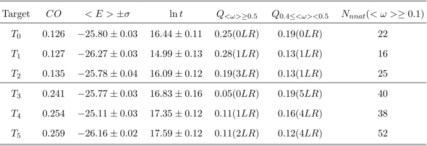
and Gutin design method [14]. The averaged trained sequence energy, < E >, and its

standard deviation, σ, are shown in Table I, where the targets are ordered with increasing

CO.

The folding dynamics was studied at the so-called optimal folding temperature, the

tem-perature that minimizes the folding time, taken as the value of the mean FPT to the target

averaged over the 100 MC runs [11]. Note that the high-CO targets are associated with

Indeed, in this 6-element target set, contact order and folding times correlate well (r = 0.84).

The simulated range of folding rates is, however, much narrower than that observed in real

proteins (≈ 5 orders of magnitude); the simulated kinetics is typical of this type of

mod-els and thus it appears to be a limitation of the lattice polymer model as well as of some

continuum, off lattice, models that exhibit similar behaviour [5].

In order to trace conformational changes we used the so-called contact map [22]. The

contact map, C, is an N ×N symmetric matrix with elements, Cij = 1, if beads i and j

are in contact (but not covalentely linked) and zero otherwise. In addition to containing the

relevant information on the protein’s structure (total number of contacts, specification of

each contact and respective range) the contact map representation provides a straightforward

way to compute the frequency, ωij =tij/t, with which a native contact ij occurs in a MC

run, tij being the total number of MC steps where Cij = 1 and t the folding time. We have

grouped the contacts into two classes, based on their frequency: If ω ≥ 0.5 the contact is

long-lived, while short-lived contacts are those with a frequency 0.4 ≤ ω < 0.5. We have

focussed on the contacts that contribute to the folding process and thus excluded from the

analysis contacts with small or marginal lifetimes.

We computed the mean frequency of each native contact < ωij >, averaged over 100

simulation runs, and report the results on Table I. We note that in the low-CO set, the

fraction of native contacts with a significant lifetime, is approximately twice as large as the

corresponding fraction in the high-CO set. In both sets, however, most of the long-lived

contacts are local (a contact is local if the contacting beads are separated by less than 10

units of backbone distance), possibly due to the local nature of the kink-jump dynamics

move set.

By contrast, the fraction of short-lived contacts is similar in both target sets; naturally

the number of long-range (LR) contacts, contributing to Q, is clearly larger in the high-CO

target set. The number of non-native contacts, Nnnat, with a marginal lifetime (ω ≥0.10) is, as expected, larger in the high-CO target set.

These results indicate that the fraction of long-lived native contacts is higher in chains

folding to low-CO targets and that, regardless of target geometry, the dynamics appears to

be dominated by local contacts as these are the most frequent. Nevertheless, the appearance

of a few long-lived LR contacts in both target sets suggests that they may play a role in the

Contact order and structural organization towards the native fold

In this section a detailed study of the folding dynamics exhibited by targetsT1 and T5 is

investigated. TargetsT1 andT5 have considerably different geometries, as suggested by their

contact order, and display the lowest and the highest observed folding times. Therefore they

are good candidates to highlight the role of the native structure’s geometry (if any) on the

folding dynamics. In particular, we investigate wether specific structural changes towards

the native fold may be identified, for a given native structure’s geometry.

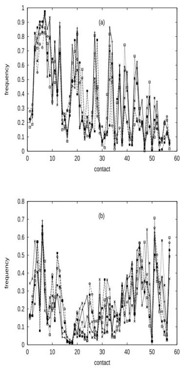
In Fig. 1 we plot the frequency, ωij, with which a native contact ij appears in the folding

simulations of six randomly chosen sequences trained for targets T1 and T5 respectively.

The major features observed for each target in different runs suggest a trend for the folding

dynamics of target T1 that is markedly different from that observed for target T5. In what

follows we will investigate this difference.

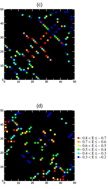
Figures 2(a) and (b) show the frequency maps of targets T1 and T5 respectively. Each

square represents an elementCij = 1 of the contact map matrix, that is, a native contactij, whose mean frequency,< wij >, averaged over 100 MC runs, falls in a certain range indicated

by the different colours. The frequency maps clearly identify the two model structures T1

andT5 and exhibit their different geometries. It is possible to identify a pattern in the colour

distribution of targetT1, which is not present in the frequency map of targetT5, suggesting

that the mean frequency of a native contact decreases monotonically with increasing contact

distance in the low-CO target.

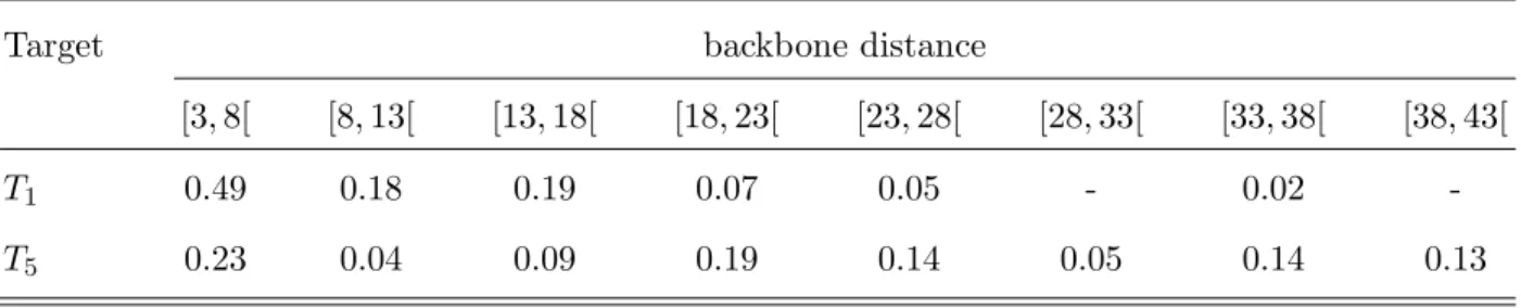
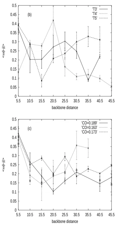
Let the backbone frequency, < ω|i−j| >, be the mean frequency < ωij > averaged over the number of contacts in each interval of backbone separation as defined in Table II. In

Figs. 3(a) and 3(b) we plot the backbone frequency as a function of the distance, |i−j|for

the targets of the low-CO and the high-CO sets respectively. While for all low-CO targets

< ω|i−j| > decreases monotonically with increasing contact distance, confirming the trend

observed in the T1 frequency map, for the high-CO targets no such trend is observed. One

possible explanation, that we have ruled out, is that of a (negative) correlation between

the frequency of a contact and its energy. In particular, one might expect the most stable

contacts, those with the lowest energy, to be the most frequent. In Fig. 2(c) and (d) we

report the energy maps of targets T1 and T5 respectively. Each square represents a native

colour. Since there is no correspondence between the colour patterns of figures 2(a) and

2(c) and between those of figures 2(b) and 2(d) we conclude that the difference is driven

by geometrical constraints. A quantitative analysis of the correlation between the contact’s

frequencies and energies yields modest correlation coefficients, r = 0.63 and r = 0.65 for

targets T1 and T5 respectively.

Let the contact time, t0, be the mean FPT of a native contact averaged over 100 MC

runs (the FPT of a native contact is number of MC steps up to the first time the contact is

formed). The contact time, averaged over the contacts in each interval of backbone distance,

are shown in Table II, and plotted in Fig. 4: In both targets the set up of local contacts

occurs largely before the LR contacts are established and, for LR contacts, there is no

correlation between the contact time and the backbone distance. In view of these results

one may be tempted to conclude that the higher folding time ofT5 is due to the fact that it

has more LR contacts. However, the folding time is non-additive and a simple calculation

shows that the higher number of LR contacts cannot justify the observed folding time ofT5.

Indeed the longest contact time (lnt0 = 12.24) is two orders of magnitude shorter than the

folding time of T5 and the sum of contact times is ln(P 57

i=1ti0) = 15.51 much lower than the

observed folding time lnt= 17.59.

From the results of Fig. 4 we infer that the average contact times, over a given range, are

similar for both targets. Thus the differences in the observed frequencies reported in Fig. 3

distinguish different cooperative behaviours.

Results obtained so far suggest that two broad classes of folding mechanisms exist for the

MJ lattice-polymer model. What distinguishes these two classes is the presence, or absence,

of a monotonic decrease of contact frequency with increasing contact range that may be

related to different cooperative behaviour. The monotonic decrease of contact frequency

with increasing contact range appears to be specific of the folding to low-CO targets. In

this case the folding is also less cooperative and seems to be driven by the backbone distance:

Local contacts form first while LR contacts form progressively later as the contact range

increases.

At this point one may ask if the different folding mechanisms identified in the previous

discussion are not a consequence of analysing only two different structures, i.e. there could

be intermediate mechanisms for intermediate native structures. In order to clarify this point,

geometries with intermediate contact order (0.163, 0.173 and 0.189) and the results are

reported in Fig. 3(c). The folding times associated with these 3 structures are 15.67±0.09,

16.46±0.09 and 16.04±0.12 and we found that the contact order and the folding times, for

the 9-element target set, correlate well (r = 0.82). The average sequence energy is in the

same range as that of the targets reported in Table I. However, it is clear from the figure

that intermediate and high-CO proteins fold via the same type of cooperative mechanism.

Contact order and the exploration of the conformational space

In this section we analyse the time evolution of the 57 native contacts of targets T1 and

T5 to obtain a picture of the ‘global’ structural changes that occur during folding.

In the folding process a chain explores conformations that may be characterised by the

fraction of native contacts, Q. Different native contacts will contribute to conformations

with the same Q. In a MC run the probability of occurrence of a certain native contact

is equal to the number of times that the contact occurs over the number of times that

conformations with a given fraction of native contacts, Q, are sampled.

Since in a given run some native contacts are more probable (or more frequent) than

others one may consider different probability intervals and ask, from the total number of

native contacts, how many occur within a given probability interval, at fixed Q. The result

gives the dependence of the number of contacts, C, on P, the probability of a contact being

formed, and onQ, the fraction of native contacts [23]. Results, averaged over 100 simulation

runs, are reported in Fig. 5(a) for T1 and in Fig. 5(b) forT5 where the coordinate Qmay be

interpreted as a monotonic ‘time’ coordinate along the folding process. Accordingly, early

folding corresponds to low-Qwhile late folding occurs at high-Q.

A first look at the figures suggests smooth dynamics for the time evolution of T1’s 57

native contacts by comparison withT5 that exhibits a considerably more ‘rugged’ behaviour.

Indeed, for a fixed probability interval, the variation, as a functionQ, of the number of native

contacts C which are present with that probability is clearly more pronounced for T5 than

for T1. This suggests that T5 does not keep a considerable number of its native contacts as

it evolves from a conformation Γ(Q) to another conformation Γ′

(Q′

) during its exploration

of the conformational space towards the native fold. A closer look shows other important

that is highly probable contacts (P ≥ 0.80), by contrast with T5 where highly probable

contacts occur only later (Q ≥ 0.50). Indeed, in the late folding of T5, there are still a

few contacts with rather low probability P ≈0.25. Moreover, as Q increases, the number

of contacts in the two highest probability intervals increases smoothly for T1, while for T5

the number of high-probability contacts shows a sudden increase only at Q ≈ 0.7. These

dynamical features are consistent with a folding scenario according to which T1 explores

more correlated native-like conformations as time evolves. ForT5, however, even though the

chain is getting more compact as it evolves towards the native fold it still explores many

uncorrelated conformations up to the late folding stage.

Contact order and non-native contacts

To investigate the effects of non-native contacts in the folding dynamics to geometrically

different native structures we have computed the dependence of the averaged number of

non-native contacts, < Nnnat >, with Q. The average is taken over 100 MC runs. Results reported in Fig. 6 show that it is possible to identify two distinct dynamical regimes: For

Q > 0.5 the number of non-native contacts decreases monotonically with Q independent

of target geometry. However, for lower Q, the dynamics is target sensitive with the

high-CO target displaying a larger number of total contacts. This data is consistent with a

folding scenario where, in the early folding of the high-CO target, conformational sampling

is geometrically restricted due to pre-existing compact structures.

Within the context of the energy landscape theory significant energy barriers, or kinetic

traps, are known to exist between compact denaturated structures slowing down the folding

process. Can the observed compact structures act as kinetic traps in the folding of T5?

In order to answer this question we have computed the transition probability curves for

both targets where the presence of plateaus indicates the presence of kinetic traps. In a

transition probability curve the folding probability, Pf old(t), is plotted againstt. Results for

targets T1 and T5 are shown in Fig. 7 where no plateaus are visible. Thus, based on these

results, one cannot claim that the longer folding time of T5 is due to the presence of kinetic

traps.

Why do high-CO structures form compact denatured states? We associate these

with a backbone separation in the range 35 ≤ |i− j| ≤ 39 and frequency in the range

0.40≤ωij ≤0.57 correspond to conformers characterized byQ ≈0.18 and a total number of contacts close to 30 (of which ≈20 are non-native). Figure 6 confirms that for Q= 0.18

target T5 is considerably more compact than target T1 that has only (≈ 12) non-native

contacts.

These findings suggest the following interpretation of the behaviour observed in Fig. 5

for the dynamics of the high-CO target’s ensemble of native contacts: The promiscuous

formation of LR contacts takes the chain through low conformational entropy states from

where it reorganises in a time consuming process towards the native fold. This major

reorganization explains why even in the late stages of folding the chain is still exploring sets

of unrelated conformations.

CONCLUSIONS AND FINAL REMARKS

In the present work we have carried out a thorough statistical analysis of the folding

dynamics of 48 mers, within the MJ lattice-polymer model, designed to high, intermediate

and low-CO target structures, in order to investigate the folding mechanisms associated

with different target geometries, and the corresponding folding rates.

We found two broad classes of folding mechanisms for the MJ lattice-polyme r model. The

main feature of the first class, that describes the folding of low-CO targets, is a monotonic

decrease of contact frequency with increasing contact range; indeed, such dependence seems

to be a specific trait of the dynamics associated with low-CO targets. The building up of

native structure is driven by backbone distance with local contacts forming first and

non-local contacts forming progressively later as contact range increases. Moreover, the analysis

of the time evolution of the 57 native contacts shows a progressive cumulative construction

of the native fold with the chain exploring more correlated native-like conformations as

time evolves. Folding to low-CO native structures is therefore gradual rather than abrupt

(or cooperative). Folding to intermediate and high-CO targets belongs to a different class,

where the dependence of contact frequency on contact range is non-monotonic. The folding

is markedly more cooperative with many high-probability contacts forming suddenly only in

the late stages of folding. Our results suggest that the higher cooperativity of the high-CO

LR contacts in the folding dynamics was obtained by Abkevich et al. in Ref. [18].

A common feature of the two folding classes is that the dynamics is dominated by local

contacts in the sense that they are the most frequent during the folding process. This feature

results, in part, from the local nature of the move set used in the simulations which favours

the formation of local contacts.

At this stage a word on the correlation between CO and foldind times is in order.

Al-though the correlation coefficient between CO and Tf for the 6 targets of Table I is high

(r = 0.82) the difference in folding times is relatively modest and this correlation should

be taken with caution. Indeed, one one includes the 9 targets studied in this work the

correlation coefficient decreases, a clear indication that these numbers are not conclusive.

However, the geometry driven cooperativity appears to be rather robust and this implies an

increase in folding times as the cooperativity increases.

Related studies, have investigated the physical mechanisms behind the (empirical)

geometry-dependent kinetics exhibited by two-state folders. Work on the ‘topomer search

model’ (TSM), concludes that the topology-dependence of real two-state folders is ‘a direct

consequence of the extraordinary cooperative equilibrium folding of simple proteins’ [24]. In

agreement with the TSM results Jewett et al. [12] showed that modified G¯o type polymers,

exhibiting enhanced thermodynamic cooperativity, display a larger dispersion of the

fold-ing rates and a stronger topology-dependent kinetics than traditional, non cooperative G¯o

polymers. In a very recent study, Kaya and Chan suggested that the way thermodynamic

cooperativity is achieved may be as important as thermodynamic cooperativity per se in

topology-dependent kinetics [5]. By studying a modified G¯o model, with many-body

inter-actions, the authors found folding rates, well correlated (r = 0.914) with CO, spanning a

range two orders of magnitude larger than that of G¯o models with additive contact energies.

The results for the modified G¯o models and our current results for the MJ model shed light

on our previous finding [11] of a particularly strong correlation (r ≈0.80) between

higher-CO structures and longer logarithmic folding rates; These structures have a larger number

of LR contacts that enhance the cooperativity of the folding transition. This cooperativity

TABLE I: Summary of target properties with targets organized with increasing contact order

parameter, CO. Targets T0, T1 and T2 constitute the low-CO target set while targets T3, T4

and T5 make the high-CO target set. < E > is the averaged trained energy and σ its standard

deviation , lnet is the logarithmic folding time, Q is the fraction of native contacts with mean

frequency < ω > (we specify the number of long-range (LR) native contacts) and Nnnat is the

number of non-native contacts with a marginal lifetime.

Target CO < E >±σ lnt Q<ω>≥0_.5 Q0_.4_≤<ω><0_.5 N_nnat(< ω >≥0.1)

T0 0.126 −25.80±0.03 16.44±0.11 0.25(0LR) 0.19(0LR) 22

T1 0.127 −26.27±0.03 14.99±0.13 0.28(1LR) 0.13(1LR) 16

T2 0.135 −25.78±0.04 16.09±0.12 0.19(3LR) 0.13(1LR) 25

T3 0.241 −25.77±0.03 16.83±0.16 0.05(0LR) 0.19(5LR) 40

T4 0.254 −25.11±0.03 17.35±0.12 0.11(1LR) 0.16(4LR) 38

TABLE II: Fraction of native contacts, Q, at consecutive intervals of backbone distance for targets

T1 and T5.

Target backbone distance

[3,8[ [8,13[ [13,18[ [18,23[ [23,28[ [28,33[ [33,38[ [38,43[

T1 0.49 0.18 0.19 0.07 0.05 - 0.02

0 0.1 0.2 0.3 0.4 0.5 0.6 0.7 0.8 0.9 1

0 10 20 30 40 50 60

frequency

contact (a)

0 0.1 0.2 0.3 0.4 0.5 0.6 0.7 0.8

0 10 20 30 40 50 60

frequency

contact (b)

FIG. 1: Frequency with which a native contact (numbered from 1 to 57) occurs in the folding

simulations of six randomly chosen sequences trained for targets T1 (a) and T5 (b). The contact

frequency is the ratio of the number of times a native contact occurs in a MC simulation to the

folding time. Note how frequency of occurence of particular contacts has strong correlation between

0 10 20 30 40 50 0

10 20 30 40 50

0 10 20 30 40 50

0 10 20 30 40 50

(a)

0 10 20 30 40 50

0 10 20 30 40 50

0 10 20 30 40 50

0 10 20 30 40 50

<ω> ≥ 0.5 0.4 ≤ <ω> < 0.5 0.3 ≤ <ω> < 0.4 0.2 ≤ <ω > < 0.3 0.1 ≤ <ω> < 0.2 0.0 ≤ <ω> < 0.1

0 10 20 30 40 50 0

10 20 30 40 50

0 10 20 30 40 50 0

10 20 30 40 50

(c)

0 10 20 30 40 50 0

10 20 30 40 50

0 10 20 30 40 50 0

10 20 30 40 50

− 0.8 < Ε ≤ − 0.7 − 0.7 < Ε ≤ − 0.6 − 0.6 < Ε ≤ − 0.5 − 0.5 < Ε ≤ − 0.4 − 0.4 < Ε ≤ − 0.3 − 0.3 < Ε ≤ −0.2

(d)

FIG. 2: (Color online). Frequency maps of targets T1 (a) and T5 (b) and energy maps of targets

T1 (c) andT5 (d). A coloured square represents a native contact with an averaged mean frequency

0 0.1 0.2 0.3 0.4 0.5 0.6

5.5 10.5 15.5 20.5 25.5 30.5 35.5 40.5

<

ω

|i-j|>

backbone distance (a)

0 0.05 0.1 0.15 0.2 0.25 0.3 0.35 0.4 0.45 0.5

5.5 10.5 15.5 20.5 25.5 30.5 35.5 40.5 45.5

< ω |i-j|> backbone distance (b) ’T3’ ’T4’ ’T5’ 0 0.05 0.1 0.15 0.2 0.25 0.3 0.35 0.4 0.45 0.5

5.5 10.5 15.5 20.5 25.5 30.5 35.5 40.5 45.5

< ω |i-j|> backbone distance (c) ’CO=0.189’ ’CO=0.163’ ’CO=0.173’

FIG. 3: The backbone frequency, < ω_|i−j| > , as a function of the backbone separation for the

low-CO (a), high-CO (b) and intermediate-CO targets (c). The backbone frequency is the mean

value of < ω > averaged over the number of contacts in each interval of backbone separation as

7.5 8 8.5 9 9.5 10 10.5 11 11.5 12 12.5

5.5 10.5 15.5 20.5 25.5 30.5 35.5 40.5

ln<t0>

backbone distance ’T1’

’T5’

FIG. 4: The averaged contact time, lne < t0 >, as a function of the backbone distance. t0 was

a

b

FIG. 5: Number of contacts, C, with a given probability of being formed, P, as a function of Q,

the fraction of native contacts for targets T1 (a) and T5 (b). These are results averaged over 100

0 5 10 15 20 25

0 0.18 0.35 0.53 0.70 0.88 1.0

<Nnnat>

Q

’T1’ ’T5’

FIG. 6: Mean number of non-native contacts,< Nnnat>, averaged over 100 MC runs, as a function

0 0.2 0.4 0.6 0.8 1

5 5.5 6 6.5 7 7.5 8 8.5 9

Pfold

log(t) ’T1’

’T5’

FIG. 7: Dependence of the folding probability, Pf old, on log10(t). Pf old was calculated as the

P.F.N.F would like to thank Dr. A. Nunes for useful discussions and Funda¸c˜ao para a

Ciˆencia e Tecnologia for financial support through grant BPD10083/2002.

∗ _{Electronic address: [email protected]}

[1] S. E. Jackson, Fold. Des. 3, 81 (1997).

[2] J. I. Guijarro, C. J. Morton, K. W. Plaxco, I. D. Campbell, and C. M. Dobson, J. Mol. Biol.

276, 657 (1998).

[3] A. R. Fersht, Proc. Natl. Acad. Sci. USA 97, 1525 (2000).

[4] P. F. N. Faisca and R. C. Ball, J. Chem. Phys.116, 7231 (2002).

[5] H. Kaya and H. S. Chan, Proteins52, 524 (2003).

[6] P. Wittung-Stafshede, J. C. Lee, J. R. Winkler, and H. B. Gray, Proc. Natl. Acad. Sci. USA

96, 6857 (1999).

[7] N. A. J. van Nuland, F. Chiti, N. Taddei, G. Raugei, G. Ramponi, and C. M. Dobson, J. Mol.

Biol. 283, 883 (1998).

[8] K. W. Plaxco, K. T. Simmons, and D. Baker, J. Mol. Biol. 277, 985 (1998).

[9] R. Du, V. S. Pande, A. Y. Grosberg, T. Tanaka, and E. Shakhanovich, J. Chem. Phys. 111,

10375 (1999).

[10] K. W. Plaxco, K. T. Simmons, I. Ruczinski, and D. Baker, Biochemistry 39, 11177 (2000).

[11] P. F. N. Faisca and R. C. Ball, J. Chem. Phys.117, 8587 (2002).

[12] A. I. Jewett, V. S. Pande, and K. W. Plaxco, J. Mol. Biol. 326, 247 (2003).

[13] L. Mirny and E. I. Shakhnovich, Proc. of the International School of Physics Enrico Fermi:

Protein Folding Evolution and Design, IOS Press p. 37 (2001).

[14] E. I. Shakhnovich and A. M. Gutin, Proc. Natl. Acad. Sci. USA90, 7195 (1993).

[15] E. I. Shakhnovich, Phys. Rev. Lett.72, 3907 (1994).

[16] A. Sali, E. I. Shakhnovich, and M. Karplus, Nature (London) 369, 248 (1994).

[17] G. Tiana and R. A. Broglia, J. Chem. Phys.114, 2503 (2001).

[18] V. I. Abkevich, A. M. Gutin, and E. I. Shakhnovich, J. Mol. Biol. 252, 460 (1995).

[19] S. Miyazawa and R. Jernigan, Macromolecules 18, 534 (1985).

[20] N. Metropolis, A. W. Rosenbluth, M. N. Rosenbluth, A. H. Teller, and E. Teller, J. Chim.

[21] D. P. Landau and K. Binder, Cambridge Univesrity Press p. 1087 (2000).

[22] S. Saitoh, T. Nakai, and K. Nishikawa, Proteins: Struct. Funct. and Genet. 15, 191 (1993).

[23] T. Lazaridis and M. Karplus, Science278, 1928 (1997).