A Thesis Submitted for the Degree of PhD at the University of Warwick
http://go.warwick.ac.uk/wrap/3159
This thesis is made available online and is protected by original copyright. Please scroll down to view the document itself.
DEGREE: . . . .
TITLE: From Gene-Expressions to Pathways
DATE OF DEPOSIT: . . . .
I agree that this thesis shall be available in accordance with the regulations governing the University of Warwick theses.
Iagreethat the summary of this thesis may be submitted for publication.
Iagreethat the thesis may be photocopied (single copies for study purposes only).
Theses with no restriction on photocopying will also be made available to the British Library for microfilming. The British Library may supply copies to individuals or libraries. subject to a statement from them that the copy is supplied for non-publishing purposes. All copies supplied by the British Library will carry the following statement:
“Attention is drawn to the fact that the copyright of this thesis rests with its author. This copy of the thesis has been supplied on the condition that anyone who consults it is understood to recognise that its copyright rests with its author and that no quotation from the thesis and no information derived from it may be published without the author’s written consent.”
AUTHOR’S SIGNATURE: . . . .
USER DECLARATION
1. I undertake not to quote or make use of any information from this thesis without making acknowledgement to the author.
2. I further undertake to allow no-one else to use this thesis while it is in my care.
DATE SIGNATURE ADDRESS
by
Ritesh Krishna
Thesis
Submitted to the University of Warwick for the degree of
Doctor of Philosophy
Supervisors: Dr. C-T Li and Prof. J.F. Feng
by
Ritesh Krishna
Thesis
Submitted to the University of Warwick for the degree of
Doctor of Philosophy
Supervisors: Dr. C-T Li and Prof. J.F. Feng
Acknowledgements xi
Declaration xiii
Abstract xiv
1 Introduction 1
1.1 Introduction ... 1
1.2 The Central Dogma of Molecular Biology ... 2
1.3 How Do Microarrays Work... 4
1.4 Time Courses vs. Independent Data Point ... 8
1.5 Data Generation and Processing ... 9
1.6 Overview of the Arabidopsis Experiment... 13
1.6.1 Material Processing and Data Collection ... 15
1.6.2 Information Processing ... 17
1.7 Road-map of the Dissertation ... 18
2 Normalization of Gene Expression Data 21 2.1 Normalization Model for the Arabidopsis Experiment ... 26
2.2 Methods ... 27
2.2.1 Select-and-Reject Method ... 31
2.3 Results ... 33
2.4 Summary ... 40
3 Functional Clustering of Gene Expression Data 43 3.1 Methods ... 48
3.1.1 Network Analysis... 52
3.2 Results ... 54
3.2.1 Illustrative Datasets... 54
3.2.2 Arabidopsis Dataset : Small Example ... 60
3.2.3 Arabidopsis Dataset : Bigger Example ... 67
3.3 Comparison With Respect to Other Existing Methods... 69
3.4 Summary ... 81
4 Partial Granger Causality 84 4.1 Methods ... 86
4.1.1 Measures of Linear Interdependence ... 86
4.1.2 Partial Granger Causality ... 88
4.1.3 Prerequisites For Causal Models ... 92
4.1.4 Bootstrap Analysis ... 93
4.2 Results ... 94
4.2.1 Illustrative Examples ... 94
4.2.2 Application to T-cell Data ... 103
4.3 Comparison With Respect to Other Methods ... 108
4.4 Summary ... 112
5 Listening to Genes 113 5.1 Methods ... 115
5.1.1 Data Generation : Overview of the Dataset... 115
5.1.2 Normalization... 116
5.1.4 Network Analysis : Complex Granger Causality... 118
5.2 Results ... 120
5.2.1 Normalization... 120
5.2.2 Frequency Analysis... 120
5.2.3 A Circadian Circuit... 124
5.2.4 Ethylene Circuit... 127
5.2.5 A Global Circuit ... 128
5.3 Summary ... 130
6 Summary and Future Work 133 6.1 Recapitulation... 134
6.2 Future Work ... 138
A Partial Granger Causality 142 B Gene Annotations 147 B.1 Gene Annotations ... 147
B.2 Gene Annotations ... 149
B.3 Gene Annotations ... 152
1.1 The central dogma of molecular biology. Figure from [Vie99]. . 3
1.2 Overview of a typical microarray experiment with two
sam-ples. Figure obtained from [Com09]. ... 5
1.3 Processing pipeline for a typical microarray experiment... 10
1.4 Arabidopsis plant. ... 14
1.5 (a) Cotton tag around leaf 7 (b) The plant images on day 1,
15 and 19 since the data collection started. Leaf 7 is marked
with an arrow. ... 16
1.6 Profiles of a leaf over 22 days during the senescence. The left
most (first) profile shows a fully developed leaf and the profile
was taken 19 days after sowing the plant. ... 16
1.7 Scanned images are read using Imagene to produce text
files with details of signal intensity and other statistics for each
gene in the image file. The text files are read to produce
quantization matrices after adjusting the gene intensity. The
quantization matrices are further combined using
normaliza-tion method to produce the final gene expression matrix for
2.1 Correlation coefficients across replicates forgbi... 34
2.2 Correlation coefficients across replicates forζgbi ... 35
2.3 Scatter plot ofgbiˆ vs. Yˆgbi... 36
2.4 Scatter plot ofζˆgbi vs. Yˆgbi ... 36
2.5 Histogram forθgbi for all the genes... 39
2.6 Original (in blue) and adjusted (in red) values for four genes across all replicates ... 39
2.7 Plots in (a)-(f) show the correlation coefficients for ζgbi be-tween the replicates for time points 1...6, whereas, plots in (g)-(l) show the correlation coefficients for θgbi between the replicates for the corresponding time points. We can see that the plots in (g)-(l) are much flatter compared to the ones in (a)-(f) ... 41
3.1 Plot of time-series for Dataset 1 ... 56
3.2 Plot of time-series for Dataset 2 ... 56
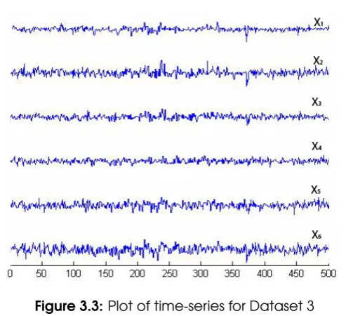
3.3 Plot of time-series for Dataset 3 ... 57
3.4 Inferred network for Dataset 1... 58
3.5 Inferred network for Dataset 2... 58
3.6 Inferred network for Dataset 3... 59
3.7 Simulation results with Dataset 1, 2 and 3 integrated into one system... 60
3.8 Temporal profiles of genes selected for smaller dataset for Arabidopsis ... 64
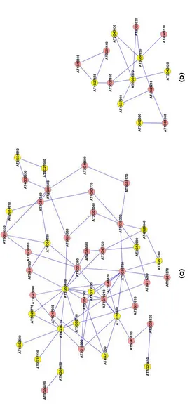
3.10 Extracted subgraphs indicating potential modules of
inter-est in the smaller dataset. Biological functions performed
by modules in respective figures are a.) Circadian rhythm
b.) Immune and Defense response c.) Circadian rhythm d.)
Ageing... 66
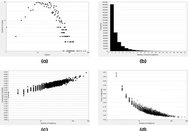
3.11 Structural properties of association network obtained for
big-ger dataset. a) A power-law like distribution obtained for
the node degree distribution. b) A distribution of number
of partners shared between a pair of nodes c) Closeness
centrality of all the nodes d) Plot for topological coefficient... 71
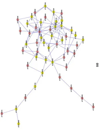
3.12 Modules 1-2 : Genes listed in Table 3.2 for network 1 (a.
Response to stress) and network 2 (b. Cytoplast) are
high-lighted with yellow. ... 72
3.13 Modules 3-4 :Genes listed in Table 3.2 for network 3 (a.
Re-sponse to stimulus) and network 4 (b. ReRe-sponse to abiotic
stimulus) are highlighted with yellow... 73
3.14 Modules 5-6 :Genes listed in Table 3.2 for network 5 (a.
Cat-alytic Activity) and network 6 (b. Response to stress) are
highlighted with yellow. ... 74
3.15 Modules 7: Genes listed in Table 3.2 for network 7 (Cell part)
are highlighted with yellow. ... 75
3.16 Two subgraphs of potential interest were detected when
correlation coefficient was used to establish association
be-tween genes in the smaller Arabidopsis dataset. ... 77
3.17 Correlation matrix for smaller Arabidopsis dataset ... 78
4.1 Network structures for the discussed examples. ... 98
4.2 Plot of PGC values for edges in the discussed examples. See
Table 4.1 for edge enumeration... 98
4.3 Detection of edges on multiple datasets. The x-axis
repre-sents the edges which were expressed for the
correspond-ing dataset on the y-axis. (a) The network in Example 1 has
edge number 10,11,12,13 and 20 expressed for most of the
datasets. See Table 4.1 for relationship between edge
num-bers and the edges. (b) Example 2 has edges 10,11,15,18
and 20 expressed for most of the datasets. (c) The network in
Example 3 has edge number 4,10,11,15,18 and 20 expressed
for most of the datasets and (d) Example 4 has edges 10,11,12,15,18
and 20 expressed for most of the datasets. ... 100
4.4 Q-Q plots for the variables in Example 1... 101
4.5 Residual plots for the variables in Example 1... 101
4.6 Q-Q plots of actual data versus predicted data after fitting
the autoregressive model. ... 105
4.7 Histogram and cross-correlation plot for innovations after
fit-ting the autoregressive model. ... 106
4.8 (a) Plot of coefficient of determination after fitting the VAR
model on T-cell data.(b) Histogram plot for the PGC values
between all pairs of genes in the dataset. ... 106
5.1 Synthesized data. A. Gene intensity vs. time. B. The
magni-tude of discrete Fourier transform of the data in A. The DC
term is not shown. C. M0 (DC term), M1 (corresponding to
the first column in B) and M11 (the 11th column in B).A clear
structure of two clusters is shown. D. The histogram of the
magnitude ofM11. ... 117
5.2 Correlation matrix of residuals before and after the
applica-tion of select-and-reject algorithm during normalizaapplica-tion (see
Chapter 2 for details). For x = 1,2,· · · ,16 is the correlation
matrix before applying the algorithm. For x = 21,22,· · ·,36 is
the correlation matrix after applying the algorithm. The
di-agonal elements of two matrices are all set to 0. ... 121
5.3 (A) Gene intensity vs. time. Only 200 genes are shown. (B)
Magnitude of all genes vs. frequency. It is clear to see that
there are two main frequencies in the data, i.e. the one of
one day period (M11, the 11th column) and the other of 22
days period (M1, the first column). The DC term M0 is not
shown. (C) Two dimensional plot of M11 vs. M1. (D) The
histogram of the DC term. There are two peaks in the
his-togram. (E) The histogram ofM1, it is a Weibull distribution. (F)
5.4 (A) Time trace of the top (in red and black) and bottom (in
blue) ten genes with the strongest amplitude of the period of
22 days. There are two classes: one is up-regulated (red thick
line), the other is down-regulated (black thick lines). (B) Time
trace of the top (in red and black) and bottom (in blue) ten
genes with the strongest amplitude of period of 1 day. There
are two classes: one is on-phase (red thick line), the other is
off-phase (black thick line). (C) Time trace of the first top (in
red) and bottom (in blue) ten genes without rhythms. Plots
in (D), (E) and (F) plot the frequency representation of top
genes in (A), (B) and (C) respectively... 123
5.5 Circadian circuits reported in literature. (a)Morning and evening
loop in Arabidopsis. From Yonovsky et al. [YK03]. (b)Morning,
evening and an unknown loop by Ueda [Ued06] (c) Inclusion
of GI gene in the circuit by Locke et al.[LKBG+06] ... 125
5.6 One gene circuit controlling circadian activity. A. Time trace
of four genes, ELF4, TOC1, LFY and CCA1. ELF4 and TOC1
are in-phase oscillators, LFY and CCA1 are in-phase
oscilla-tors, but they are off-phase oscillators with respect to ELF4
and TOC1. B. Magnitudes vs. frequency for the four genes.
They have highest magnitude at the frequency of one-day
period. C. The gene circuit obtained in terms of PGC (see
annotation in Supplemental material II). D. Complex
interac-tions between different group of genes and GI. D. Gene
5.7 A. An ethylene gene circuit with 16 genes. Only genes with
interactions are shown here. The thick arrow is the complex
interaction between CTR1, ETR1 and ERS2 and EIN2. B.
Inter-actions in the frequency domain calculated in terms of PGC.
Only 14 significant interactions are shown... 129
5.8 Causal relationship between genes: a global circuit. A. A
total of 11 genes are shown and a clear hierarchy structure is
Writing one’s PhD research in a comprehensive document like this, rigorously
and repeatedly tests the claim made by the famous American essayist Ralph
W. Emerson: “sometimes a scream is better than a thesis”. One can not bring
the endeavor of PhD research to this stage and maintain the sanity without the
precious support of supervisors, friends, and family.
The work reported in this thesis could never have been completed without the
precious support of my supervisors Prof. Jianfeng Feng and Dr. Chang-Tsun Li.
I am thankful to both of them not only to guide me throughout my research,
but also to give me the confidence that they are ever present, and nothing could
go wrong. More importantly, I am indebted to both of them to help me in the
time when I really needed the help, both professionally and personally. I will
always remember those gestures fondly and gratefully. I am also grateful to Dr.
Vicky Buchanan-Wollaston for providing the biological data used in this study
and explaining many valuable concepts. Very special thanks to Prof. Dongyun
Yi for many stimulating discussions and contribution to my research.
I am thankful to the staff members of department of computer science for
ensuring that the students face the least administrative problems during their
research. In particular, I am grateful to our head of department Prof. Roland
A huge thanks to my friends in Oxford, Dr. Amol Patil and Mrs. Monica
Mantri, for sheltering me in their home during the whole period of the thesis
writ-ing. The homely comforts and their warmth continuously challenged the above
quoted claim by Mr. Emerson. This document would have taken much longer if
they had not stepped in time to pick me up and bring to their lovely nest. My
friends Ashutosh Trivedi and Tiziana Faveretto also deserve a grateful
acknowl-edgment for the similar reasons. One can feel incredibly lucky to have two houses
in Oxford, while still being a research student, that too the one who is writing his
PhD thesis !!
I would like to thank my friends Rajesh Balakrishnan, Nikolaos Papanikolaou,
Anil Sorathiya, Dr. Estelle Guyez, Marie Clucas, Michal Rutkowski, Agnieszka
Rutkowska, Daniel Alejandro Valdes Amaro, Antony Holmes, Dr. Ashutosh, Jothi
Philip, Tina Thomas and Mirela Domijan for continuously providing their
sup-port and encouragement throughout my PhD. I am also thankful to many of my
other friends and colleagues at University of Warwick to make my life easier and
enjoyable.
Last, but not the least, my sincere thanks to my ever supporting parents and
This thesis is presented in accordance with the regulations for the degree of Doctor
of Philosophy. It has been composed by myself and has not been submitted in any
previous application for any degree. The work in this thesis has been undertaken
by myself under the joint supervision of Dr. C-T. Li and Prof. Jianfeng Feng.
Although the key findings of the thesis have been announced in an international
journal and proceedings of some international conferences, this thesis presents the
results with more details and complements them with illustrations. Chapter 2 and
Chapter 5 are the extended versions of the paper “Listen to Genes: Dealing with
Microarray Data in the Frequency Domain” [FYK+09], which appeared in the
journal PLoS ONE 2009. Chapter 3 is an extended version of the paper
“Interac-tion Based Func“Interac-tional Clustering of Genomic Data” [KLBW09], which appeared
in the proceedings of the IEEE International Conference on Bioinformatics and
Bioengineering(BIBE) 2009. Chapter 4 is an extended version of the paper “A
partial Granger causality approach to explore causal networks derived from
multi-parameter data” [KG08], which appeared in Lecture Notes in Computer Science
(LCNS) 2008. Two more manuscripts have been prepared from the materials in
Chapter 3 and Chapter 4 in this thesis and have been submitted to international
Rapid advancements in experimental techniques have benefited molecular biology
in many ways. The experiments once considered impossible due to the lack of
resources can now be performed with relative ease in an acceptable time-span;
monitoring simultaneous expressions of thousands of genes at a given time point
is one of them. Microarray technology is the most popular method in biological
sciences to observe the simultaneous expression levels of a large number of genes.
The large amount of data produced by a microarray experiment requires
consid-erable computational analysis before some biologically meaningful hypothesis can
be drawn. In contrast to a single time-point microarray experiment, the temporal
microarray experiments enable us to understand the dynamics of the underlying
system. Such information, if properly utilized, can provide vital clues about the
structure and functioning of the system under study. This dissertation introduces
some new computational techniques to process temporal microarray data. We
fo-cus on three broad stages of microarray data analysis - normalization, clustering
and inference of gene-regulatory networks. We explain our methods using various
synthesized datasets and a real biological dataset, produced in-house, to monitor
Introduction
1.1 Introduction
Over the last ten years or so genome sequencing has made rapid progress. Genome
sequencing has facilitated transfer of information from DNA of a species to
elec-tronic computers. Identification and symbolic representation of correct genes are
only the preliminary goals of genome sequencing, the holy grail of biology lies in
understanding the functions of those genes. This has given birth to a new research
field known as functional genomics.
Much of the success in genome sequencing can be accredited to high
through-put DNA sequencing techniques. This led to what primarily used to be a wet
science to become in larger part an information science [Qua07]. Similar high
throughput techniques have been developed for functional genomics also. Most
notable among them are DNA microarray technologies. Microarrays allow
re-searchers to monitor simultaneous gene expression levels of thousands of genes in
an organism in a single experiment. On one hand, advancing experimental
tech-niques are producing tons of data which can provide clues about the functions
mean-ingful information from that data and build biological hypotheses which can be
tested in laboratories. The development of computational methods and tools to
analyse such massive data is the task of computational biology and bioinformatics.
This dissertation addresses some of the challenges found in analysis of
mi-croarray data and provides techniques to address them. We provide a complete
pipeline for dealing with three broad stages in microarray data analysis, namely,
normalization, clustering and inference of gene regulatory networks. Our goal is
to automatically infer the meaningful signals using statistical techniques and build
plausible biological hypotheses for further testing in the laboratory.
1.2 The Central Dogma of Molecular Biology
To understand how gene expression works, we need to understand the Central
Dogma of biology. Cells are fundamental working units of every living
organ-ism. Cells are largely made of proteins which define their shapes and structures.
Proteins are functional molecules essential for performing many life functions like
catalysis, signalling etc. The central dogma of biology charts out the flow of
infor-mation from DNA molecules to proteins. DNA is a stable molecule containing the
complete genetic blueprint of living organisms. The information in DNA is stored
as a code made up of four chemical bases known as nucleotides : adenine (A),
guanine (G), cytosine (C), and thymine (T). Segments of DNA known as genes
are transcribed into messenger RNA(mRNA) which are subsequently translated
into proteins. This complete process is known as gene expression.
Figure 1.1 presents a pictorial representation of the stages involved in the
cen-tral dogma. There are three broad stages in the inheritance of genetic information
The Central Dogma of Molecular Biology
Replication
DNA duplicates
Transcription
RNA synthesis
Translation
Protein synthesis DNA
Information
Information
mRNA RNA polymerase Nucleus
Cytoplasm
Nuclear membrane
mRNA ribosome
protein
Protein RNA
[image:22.595.183.414.139.409.2](Andy Vierstraete 1999)
Figure 1.1:The central dogma of molecular biology. Figure from [Vie99].
DNA creates identical copies of itself and the genetic information is replicated. A
segment of DNA called agenecontains both coding sequences that determine the
function of the gene, and non-coding sequences that determine when the gene is
active (expressed). When a gene is active, the second stage in the central dogma
named astranscriptiontakes place, where the coding and non-coding sequences of
the gene are copied to produce a single stranded RNA copy of the gene’s
informa-tion. The RNA moves from the nucleus into the cytoplasm where the ribosomes
are located. There are multiple types of RNAs in nature, but the one
responsi-ble for protein coding is known as messenger RNA or mRNA. The mRNAs are
trans-lation, the mRNA sequence is translated into a sequence of amino acids as the
protein is formed. The translation of mRNA to protein is performed by ribosomes
which read three bases (a codon) at a time in the mRNA sequence and translate
them into one amino acid according to the rules specified by genetic code.
A key consideration is that all the cells in an organism’s body contain the
same copy of DNA molecule, yet all the cells are not same. The diversity is
due to the difference in gene expressions across different cell types. Different gene
subsets which eventually lead to different proteins synthesized, express themselves
in different ways by reflecting both the cell types and their conditions. Microarrays
quantify the gene expressions by monitoring the abundance of mRNA molecules
during the transcription stage. The amount of each mRNA detected in the cell
can provide information on the level of expression for the corresponding gene.
1.3 How Do Microarrays Work
Microarray technology is based on the principle ofDNA hybridization, a process in
which DNA strands bind to their unique complementary strands. A DNA molecule
consists of two complementary strands, each strand containing the information to
describe the other (adenine(A) bonds only to thymine(T), and cytosine(C) bonds
only to guanine(G)). A microarray is typically a solid surface of either glass or
silicon chip. A set of specific DNA oligonucleotides, or cDNA, or small fragments
of PCR (polymerase chain reaction) products corresponding to mRNAs (these all
are collectively called known sequences) are attached on the solid surface at fixed
locations using covalent bonds. The choice of oligonucleotides, cDNA, or PCR
products depends on the manufacturers of the arrays. The immobilized known
sequences are also called probes. The fluorescently tagged targets (unknown
Figure 1.2: Overview of a typical microarray experiment with two samples. Figure ob-tained from [Com09].
significant sequence complementarity. After allowing sufficient time for the
hy-bridization to take place, the excess sample is washed off the solid surface. The
binding affinity of each probe with the labelled target reflects the proportion of
the expression of the gene represented by that probe. Hybridized microarrays are
excited by a laser and scanned at suitable wavelength for detection of fluorescent
dyes to estimate the amount of intensity bound to each probe. The intensity
measured at each probe is an indicator of the expression level of the gene on that
array, which after adjustment for technical artefacts, should provide an estimate
of the level of gene expression which can be used for further analysis.
Microarrays can be used to measure gene expressions in different ways. One of
samples representing the same cells or cell types under two different conditions.
In this case, the mRNA extracted from each sample is labelled differently, for
instance, a green label (using the fluorescent dye Cy3 having the fluorescence
emission wavelength of approximately 570 nm) for the sample from condition 1,
and a red label (using the fluorescent dye Cy5 having the fluorescence emission
wavelength of approximately 670 nm) for the sample from condition 2. Both the
Cy-labelled samples are mixed and hybridized on a single array. The hybridized
array is scanned at the suitable wavelengths to produce separate expression
pro-files for Cy3 and Cy5 tags. Figure 1.2 shows steps in a typical microarray
exper-iment involving two sample types. Such experexper-iments typically rely on the ratio
based analysis of relative intensities of samples to identify up-regulated or
down-regulated genes.
Another popular variation of microarray experiment involves hybridization of
single-labelled population of samples to each array. In this case, the experiments
give estimations of the absolute level of gene expressions. If we want to compare
gene-expressions for two different samples, we need to perform two separate
single-label experiments and compare the absolute gene-expression levels. In this case,
comparisons are primarily made between the data obtained from different arrays,
as opposed to between the labelled populations hybridized to a single array. The
experiments with two-colour labels are also known as two-channel experiments.
On the same lines, the single-colour experiments are known as single-channel
experiments. An advantage of single-channel experiments over two-channel
ex-periments is that the absolute value of gene expressions may be easily compared
between studies from different experiments conducted months or years apart. At
the same time, it is possible to treat a two-channel experiment as a single-channel
than relying on the intensity ratios of spots between samples.
Microarrays are useful in a wide variety of studies to achieve wide variety of
objectives. The objectives can be broadly divided into four categories
-1. Class comparison - Involves comparison of gene expression profiles among
samples selected from predefined classes to identify the differentially
ex-pressed genes,
2. Class prediction - Similar as class comparison, but requires building a
sta-tistical model to predict the class of a new specimen based on its expression
profile,
3. Class discovery - Involves the identification of novel subtypes of specimens
within a population. In context of drug discovery, class discovery methods
can be used to find putative (sub-)types of diseases and to identify
informa-tive subsets of genes with disease-type specific expression profile,
4. Pathway analysis - Involves identification of co-regulated genes, or the ones
which belong to the same biochemical pathway.
Microarrays were first used to study global gene expressions in Saccharomyces
cerevisiae in 1997 by DeRisi et al. [DIB97]. A genome-wide measurement of
tran-scription is called an expression profile and provides us with a complete list of
genes whose transcription level is affected in a given condition. In a biological
sense, what we measure is how the gene expression of each gene changes to
1.4 Time Courses vs. Independent Data Point
There are two types of microarray datasets : time-independent (or single point
steady-state), and time-series(time dependent) datasets. The majority of the
mi-croarray experiments are carried out for pair-wise comparison between different
samples at a single time-point. It is relatively easy to compare and contrast
single-point datasets belonging to different experimental conditions to identify the sets
of differentially expressed genes across conditions. However, to verify that the
ob-tained results are reliable and robust to variations in the experimental procedure,
it is necessary to repeat a given experiment several times independently. Thus,
a successful comparison for time-independent datasets requires several
indepen-dent repetitions of the experiment in which the different conditions are tested in
parallel. In general, the time-independent gene expression profiles are capable of
recovering steady-state behaviour of the system, but fail to recover the temporal
regulating relationships.
Time course experiments, on the other hand, can improve the inference greatly
in contrast to time-independent data sets [ZSD06]. Time course experiments have
been proven to be useful in a number of experimental systems, providing
informa-tion about the difference in each transcript over different time points, reflecting
information about the order of events and their trends. Another main advantage
of the time-course experiment is that samples for a given experiment are all
de-rived from a single relatively homogeneous population, making the results much
less sensitive to the population-specific effects or the slight differences in the
ex-perimental or biological background. The time points at which mRNA samples
are taken are usually determined by the investigator’s judgement concerning the
Time course experiments can be further classified into two categories :
peri-odicanddevelopmental. Periodic time-courses include natural biological processes
whose temporal profiles follow regular patterns. Examples are cell cycles [SSZ+98],
circadian rhythm [HHS+00, CCWN+01] etc. In developmental time course
exper-iments, gene expression levels are measured at successive times, depending on the
timing of phenomena of interest, during the developing phase, for example ,
nat-ural growth or decay [TBW+02, HVV+04] in a cell type. Such experiments are
also useful in understanding effect of controlled stimulus in a given system, for
example, the effect of drug treatment on a cell type over a period of time.
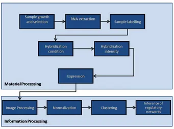
1.5 Data Generation and Processing
Collection and analysis of data in any high-throughput experiment like microarray
can be performed in two major stages :
1. Material processing and data collection stage, and
2. Information processing stage
The material processing and data collection stage is concerned with the lab based
activities related to the biological samples and experimental instruments, and can
be further broken down into the following steps
-1. preparation of biological samples to be studied;
2. extraction of RNAs from the samples;
3. labelling of RNAs using fluorescent dyes;
5. excitation of arrays by laser at suitable wavelength to detect the
hybridiza-tion intensity;
[image:29.595.132.473.204.457.2]6. scanning the hybridized array to produce image files.
Figure 1.3:Processing pipeline for a typical microarray experiment.
The information processing stage is essentially computer based analysis of the
data and can be broken down into four distinct steps
-1. image processing of the scanned images to extract gene expression levels;
2. normalization of gene expression values;
3. clustering of genes;
4. inference of regulatory networks.
A systematic diagram for the order of steps in each stage can be seen in
of this thesis. The steps need to be performed in a sequential order as shown in
the pipeline in Figure 1.3 before some meaningful hypothesis from data can be
derived. We present a brief description of the steps in the information processing
stage
- Image processing - The digital images obtained from microarray experiments
need to be analysed in order to gain information about gene expression
lev-els. Each spot on the array is identified and its intensity is measured and
compared with the background. Image quantification is usually performed
by image processing software which sometimes are provided by microarray
manufacturers. The image quantification software extract the data from
digitalized images and combine in a table commonly known as the image
quantization matrix. Each row represents one spot on the array, and each
column represents different quantitative characteristics like mean or median
pixel intensity for that spot. Image quantification for microarray
experi-ments is not a trivial task and can be regarded as an area for experts.
Normalization - The data from multiple hybridizations or different arrays in
theimage quantization matrix must be further analysed and should be
com-bined into agene expression matrix. In thegene expression matrix, each row
represents a gene and each column represents a particular biological
sam-ple or experimental condition. The combination of information from image
quantization matrix to gene expression matrix is not a trivial task. There
are several experimental artefacts which must be taken into account while
doing the conversion. There are many biological and experimental variations
which can affect the expression level of each spot. The biological samples
and the experimental conditions may differ across different arrays, and
ob-taining a single value for each gene can require considerable attention. The
values across spots. There are many methods for microarray normalization
but there is no standard fitting all the cases. The data normalization is very
much dependent on the platform, experimental setup and practitioner’s
hy-pothesis. Once the data has been normalized properly, we use values in the
gene expression matrix for further analysis and data mining.
Cluster Analysis - The next step after data normalization is to group the
genes based on certain features which help in reduction of data dimension.
The goal of clustering techniques is to discover the underlying gene pathways
representing the biological processes. Genes lying in the same pathway are
often activated or depressed simultaneously or sequentially upon receiving
stimuli. Clustering can help in recognizing biologically relevant patterns
among genes. The importance of clustering is more apparent while dealing
with a large number of genes. Automated grouping of genes in several
clusters on the basis of structural or functional similarity can substantially
help in recognition of genes of interest, and thus, can reduce the amount of
data to be analysed further.
Inference of regulatory networks - The ultimate goal of microarray
experi-ments is to understand the interactions among genes. Understanding the
in-teractions can help unlock the functioning and behaviour of genes leading to
development of potential therapeutic targets and drug discovery. Gene
reg-ulatory networks are indicators of networks among genes and are concerned
with the control of transcription i.e., how genes are up or down regulated
with respect to different signals. Inference or reverse-engineering of gene
regulatory networks from data is a step downstream to cluster analysis in
the microarray information processing pipeline. Reverse-engineering refers
choice of computational methods for creating the models depends crucially
on the kind of modelling techniques used. The models can produce further
hypothesis which can be verified in additional laboratory experiments.
1.6 Overview of the Arabidopsis Experiment
Much of the work in this dissertation is explained and tested with the microarray
data produced by scientists at Warwick Horticulture Research group at the
Uni-versity of Warwick, UK. The experiment was performed to study the process of
senescence in leaves of Arabidopsis thaliana over a period of time.
Arabidopsis thaliana (also known as thale cress, mouse-ear cress or
Arabidop-sis) is a small garden weed type flowering plant. Although not an economically
important plant, Arabidopsis has become popular as a model organism in plant
biology due to its genome being one of the smallest among other plant genomes.
It was also the first plant genome to be sequenced. Arabidopsis has several traits
that make it a useful model for understanding the genetic, cellular, and molecular
biology of flowering plants. Arabidopsis has a short life cycle of about 8-10 weeks
and it can grow about 50 cm in height in as little as 1cm3 of soil. The small
size and the rapid life cycle of the plant are advantageous for research. It can be
grown in a small space and it produces many seeds. Each of these traits leads to
Arabidopsis being a model plant organism for plant biologists.
The primary goal of the project undertaking the biological experiment
ex-plained in the following sections was to understand the senescence process in
leaves of Arabidopsis. Senescence is a term for the collective process that leads
to the ageing and death of a plant or a plant part, like a leaf. In the case of
Figure 1.4: Arabidopsis plant.
senescence is well differentiated from ageing which is a passive time-dependent
degenerative process. Senescence in a plant, on the other hand, is an internally
regulated developmental process based on an adoptive mechanism, and the death
is its consequence. The basic molecular mechanism of senescence both in plant
and animal systems may be the same. Senescence can take place due to natural
reasons, or due to environmental stress factors. The process involves expression
of specific genes. As for example, plants undergo the process of leaf senescence to
prepare for winter and recycle some of the valuable and scarce mineral nutrients.
Leaf senescence is also a mechanism to get rid of old and photosynthetically less
efficient leaves in the evergreen plants.
In Arabidopsis, leaf senescence is a programmed cell event responding to wide
range of external and internal signals. The leaf senescence in Arabidopsis is
and therefore, leaves that develop later in life, will senesce later. In addition to
age, plant hormones and environmental conditions can modulate the progression
of leaf senescence [Sma94, Pes05]. The process, however, is not only concerned
with death alone, but involves several events associated with massive
mobiliza-tion of nutrients in a highly ordered and regulated manner from senescing leaves
to new leaves, seeds and buds, thus contributing to the nutrient cycling. Many
different genes show enhanced expressions during senescence process, and can
help elucidate the underlying signalling pathways. Identification of the key genes
and pathways can result in understanding the mechanisms that occur during the
senescence process. Although, the leaf senescence alone can not explain the
senes-cence process in the whole plant, but can provide vital clues for understanding
senescence as a whole process.
1.6.1 Material Processing and Data Collection
The experiment was performed over 40 days with the following steps involved in
the material processing and data collection stage.
Plant growth and leaf material acquisition: Arabidopsis plants (Columbia
seed type also known as COL-0) were grown in a controlled environment
at 20oC temperature , 70% relative humidity and 250µ mol m−2s−1 light
intensity. The plants were subjected to long days with 16 hours of sunlight.
The seventh leaf (leaf 7) on its emergence during the development of each
plant was tagged with a cotton around it. Figure 1.5 (a) shows a cotton
tagged leaf. The cotton tags would act as identifiers later in the
experi-ment. Four such leaves were selected for harvesting purposes. After 19 days
from sowing, when the leaf 7 was fully developed, it indicated the beginning
of the time course. The biological replicates were harvested both in morning
days. Figure 1.5(b) shows the plant growth on day 1,15 and 19 since the
data collection started. Figure 1.6 shows the development of leaf 7 from
fully developed until fully senescent. This resulted in total 22 time point
samples for each leaf.
(a) (b)
Figure 1.5:(a) Cotton tag around leaf 7 (b) The plant images on day 1, 15 and 19 since the data collection started. Leaf 7 is marked with an arrow.
Figure 1.6: Profiles of a leaf over 22 days during the senescence. The left most (first) profile shows a fully developed leaf and the profile was taken 19 days after sowing the plant.
RNA isolation and probe preparation: RNA was isolated from 4 individual
leaves as separate biological replicates using the Triazol method (Invitrogen)
followed by RNeasy column purification (Qiagen). RNA was amplified using
a MessageAmp II (Ambion) and then labelled with Cy3 or Cy5 using reverse
transcriptase (SuperScript II, Invitrogen). Each amplified RNA sample was
labelled twice with Cy3 and twice with Cy5 giving 4 technical replicates for
each leaf sample. Two Cy3 and Cy5 labelled samples (in 25% formamide,
5x SSC, 0.1% SDS and 0.5 mg ml−1 yeast tRNA) were mixed in different
Hybridization: The microarrays used for analysis of the samples were
Com-plete Arabidopsis Transcriptome Micro Arrays (CATMA). Each array
con-tains 30,336 gene probes belonging to the genome of Arabidopsis. These
arrays are produced by Warwick HRI using a sterile spotting machine. The
description of the machine and the array can be found in [LKB+07]. These
arrays were hybridized with labelled samples at 42oC overnight. Slides were
washed and then scanned using an Affymetrix 428 array scanner at 532nm
(Cy3) and 635nm (Cy5).
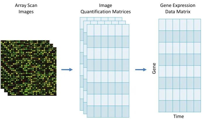
1.6.2 Information Processing
Array Scan Images
Image Quantification Matrices
Gene Expression Data Matrix
Time
[image:36.595.125.473.378.583.2]Gene
Figure 1.7:Scanned images are read using Imagene to produce text files with details of signal intensity and other statistics for each gene in the image file. The text files are read to produce quantization matrices after adjusting the gene intensity. The quantization matrices are further combined using normalization method to produce the final gene expression matrix for further data analysis.
was performed using Imagene version 7 software (BioDiscovery, http://www.
biodiscovery.com/). Figure 1.7 presents a schematic diagram of obtaining a
final gene expression matrix from scanned image files. We have one scanned
dig-ital image file (.tiff format) for each replicate at each time-point. The image files
were read using the Imagene software to produce text files with signal intensity
values for the genes, along with other statistics like background mean, median etc.
The quantified values for all the replicates were further adjusted and combined to
produce a final gene expression matrix. The process to produce the gene
expres-sion matrix from quantification matrices is called normalization. The expression
values in the final gene expression matrix will be used for the remaining stages in
the information processing pipeline. The normalization step to produce the final
gene expression matrix along with the other steps in the information processing
stage are explained in greater details in later chapters.
1.7 Road-map of the Dissertation
This chapter presented an overview of the microarray technology and explained
the experiment performed to understand the process of senescence in
Arabidop-sis leaves. The main focus of this dissertation is on the development of statistical
techniques for the last three steps in the information processing stage in a
microar-ray experiment, last three steps being normalization, clustering, and inference of
regulatory networks.
The immediate step after the image analysis in the information processing
stage of microarray is to clean the data from unwanted experimental variations,
and combine the expressions collected from different arrays to produce a single
gene expression matrix. Chapter 2 presents a normalization method to deal with
us-ing a statistical error model and different sources of experimental variations are
estimated. The method further uses an iterative algorithm to minimize the
cor-relation among the residual terms across replicates.
The normalized data is clustered according to the temporal profiles of genes in
Chapter 3. Clustering assigns genes into groups based on their related expression
patterns; such groups contain functionally related genes or genes that are
co-regulated. We adopt a Granger causality based temporal-precedence technique
to cluster the Arabidopsis genes. The association graph showing the connectivity
between various genes is analysed using a graph-theoretic method to detect dense
regions in the graph. The dense regions could be indicators of the biologically
relevant complexes. The genes in the subgraphs representing the dense regions
are queried against publicly available Gene Ontology database to test for the
func-tional similarities between genes.
In Chapter 4, we present a reverse-engineering technique to infer gene
cir-cuits from temporal microarray data. We extend the Granger causality technique
presented in Chapter 3 to infer directional network structures from gene data
in a multivariate context. We name this technique Partial Granger Causality
(PGC). Partial Granger Causality is tested using various artificial datasets
repre-senting different scenarios of connections among the participating entities. Partial
Granger Causality is further applied to a publicly available dataset for Human
T-cell activation. We apply Partial Granger Causality to infer gene circuits from
the Arabidopsis data in chapter 5.
Chapter 5 brings the techniques discussed in previous chapters together and
normalization to the inference of selected gene circuits. Chapter 5 also introduces a
frequency based analysis for the Arabidopsis dataset to detect interesting patterns
in the frequency domain. The Partial Granger Causality discussed in chapter 4 is
extended to infer interactions between sets of genes, and the extended technique is
called Complex Granger Causality. Three gene circuits, namely, circadian,
ethy-lene, and a global gene circuit are inferred using Partial and Complex Granger
Causality.
In the last chapter, we summarize the work done in each chapter. We conclude
with a discussion on the possibilities of improvements in the proposed methods
Normalization of Gene Expression
Data
Microarray technologies provide a powerful mechanism to simultaneously detect
and measure expression levels for tens of thousands of genes in a single
experi-ment. The vast quantity of data if suitably analysed can help in understanding
cellular processes, diagnosis of diseases and development of potential
therapeu-tic targets. The effective analysis of the experimental results relies on the good
quality of data. Experimental variations such as design of arrays, mRNA
qual-ity, labelling and dye effects, hybridization conditions, human and machine errors
in the scanning process contribute towards obscuring variations found in a
Mi-croarray data. To overcome these obscure variations, and make the observations
from different arrays comparable, an effective normalization technique is required.
The beginning point of any normalization method is reading the digital image
files and forming the image quantization matrices. The gene-expression values in
the matrices then need to be adjusted to produce cleaner data for further analysis.
Image processing softwares like GeneSpring [gen09], Imagene [ima09] etc. analyze
typ-ical measurements reported are total intensity, mean, median and mode of pixel
intensity distribution, as well as an estimate of these for the local background,
and other statistics such as the standard deviation of both signal and background.
Once the appropriate adjustments have been made during image analysis to
pro-duce the quantization matrices, the process of normalization begins to adjust the
gene values for different systematic biases. Normalization techniques differ
ac-cording to microarray platforms and designs of experiments. We discuss mainly
the normalization techniques used for two-channel or two-colour (red and green)
microarray platforms in this chapter.
The objective of normalization is to adjust the gene expression values of all
genes on the array to remove experimental artefacts. All normalization methods
are based on some underlying assumptions about the data and the experimental
design, and consequently, the normalization approach used must be appropriate
to the particular experiment in consideration. In a typical microarray experiment,
there are two decisions to be made for normalization : which genes to use as
nor-malization genes, and which nornor-malization algorithm to use.
Normalization approaches typically use either the complete set of arrayed genes
or a control set of genes, generally, either a set of housekeeping genes or a set of
spiked-in genes. Housekeeping genes are the ones that are involved in essential
activities of cell maintenance and survival, but that are not involved in cell
func-tion or proliferafunc-tion. Because all cells need to express these genes to survive, it
is reasonable to expect that such genes will be similarly expressed in all samples
in the experiment. Unfortunately, it is often difficult to identify housekeeping
genes, also, there is a accumulating evidence that many of these genes change
the other hand are realized by including in all the samples some RNA which is
generally not found in either sample. For example, adding some yeast RNA in
human samples. By placing some relative amount of RNA into all the samples, it
is possible to create an artificial set of housekeeping genes which will have same
expression across both the channels in a two-colour microarray experiment. The
problem with this method is that it is necessary that the proportion of sample
RNA of spiked RNA must be the same in both the channels. This is a technically
challenging problem.
Once a normalization gene set has been selected, a normalization factor is
calculated for each gene and is used to adjust the data to compensate for the
experimental variability. The key consideration in normalization methods involves
determination of the amount by which the genes in the red channel change relative
to the genes in the green channel. The bias can differ from array to array and
gene to gene. Once the size of the bias is estimated, we obtain the final signal
value by subtracting the normalization factor from the observed log ratio of genes
between two channels. The normalization algorithms to estimate this bias can be
categorized in three categories :
1. Linear or global normalization
2. Intensity based normalization, and
3. Location based normalization
Linear or global normalization assume that the red and green intensities have
a linear relationship for the normalization genes on a given array. The slope of this
linear relationship will determine the amount of normalization required. Since a
single parameter is used to scale the whole data, this type of normalization
normalization technique are, log centering, rank invariant methods [TRLW01],
quantile-based method [BIAS03], linear regression approach [CP91], and Chen’s
ratio based method [CDB97] etc. Yang et al.[YDLS01] summarized a number of
normalization methods for global normalization in their publication.
Another group of normalization techniques called intensity based
normaliza-tion methods consider that the overall magnitudes of the spot intensity may have
an impact on the relative intensities between the channels. This claim is assessed
using so-called M-A plots proposed by Yang et al. [YDLS01, YDL+02]. Locally
weighted linear regression (LOWESS) analysis has been proposed as a
normaliza-tion method that can remove such intensity-dependent effects [YDL+02, Cle79].
Kepler et al. [KCM02] proposed a local regression to estimate normalized
inten-sities as well as intensity dependent error variance. Smyth et al. [SS03b] present
a comparison of methods used for intensity based normalization methods.
An artefact that is sometimes observed is that the background subtracted
log-ratios on an array varies in a predictable manner based on their position on
the array. Such artefacts could appear due to the difference in print-tips used
to create the slide. In order to perform such location based normalization, it
is necessary that there be significant number of normalization genes within each
grid. A non-linear LOWESS normalization for correcting spatial heterogeneity
was proposed by Edward [Edw03]. Chen et al. proposed a normalization method
to adjust for location based biases combined with intensity biases [CKS+03]. Fan
et al. [FTVWY04, FHP05] have presented error model based iterative algorithms
to estimate the print-tip effects on two-colour microarrays.
nor-malization techniques with reference samples. See [Qua01, Qua02, PYK+03] for
a detailed review of the subject.
Much of the above techniques depend on the experimental designs where
ref-erence gene sets are available, which serve as a basis for comparison between
samples. Another class of popular normalization techniques which do not utilize
common reference samples have been studied using statistical error models. The
experiments which do not compare two samples, or do not use reference samples,
the log ratios of channel intensities do not need to be representative of
expres-sion level of genes on an array. Instead of taking log ratios, the analysis must
be based on channel specific intensities. Models of this type have been suggested
by Kerr and Churchill [KKC00, KC01], Wolfinger et al. [WGW+01], Dobbin et
al. [DSS03] etc. Such models explicitly include various factors of variations like
sample bias, dye bias, array bias etc. and are fitted for each gene on the array.
As an example, we present a model presented by Kerr and Churchill [KKC00]
to help understand this concept. Assume that a microarray experiment involves
multiple arrays. Every measurement in the microarray experiment is associated
with a particular combination of an array, a dye (Cy3 or Cy5), a variety type, and
a gene. Letyijkg denote the log value of measurement from theith array,jth dye,
kth variety type, and gth gene. To account for the multiple sources of variation
in a microarray experiment, they formulated the model in the following way :
yijkg =µ+Ai+Dj +Vk+Gg+AGig+V Gkg+ijkg
Here, µdenotes the overall average signal, Ai represents the effect ofith array,
Dj represents the effect of jth dye, Vk represents the effect due to the kth verity
type,Gg represents the effect of thegth gene,AGig represents the effect due to the
kth verity and gth gene. The error terms ijkg are assumed to be independent
and identically distributed with mean 0. All of the above effects may not be
of general interest but account for sources of variations in the microarray data.
It is possible to include other effects as well in the model based on the requirement.
Although, there are many methods for microarray normalization but there is
no standard fitting all the cases. The data normalization is very much dependent
on the platform, experimental setup and practitioner’s hypothesis. Also,
normal-ization alone cannot control all systematic variations but plays an important role
in microarray data analysis. The adjusted expression data can significantly vary
with different normalization procedures. Subsequent analyses, such as detection
of differentially expressed genes, clustering and inference of gene networks depend
a lot on the quality of data obtained after normalization [PYK+03].
2.1 Normalization Model for the Arabidopsis Experiment
To understand what could be a suitable model for normalization for the
Arabidop-sis data discussed in section 1.6, let us summarize the scenario again. We collected
data from 4 leaves, each one provided us a biological sample at each time point.
RNA samples were extracted from each leaf which were labelled twice with Cy3
and twice with Cy5, providing 4 technical replicates for each biological sample.
The data has been collected over 22 days. The main aim of the experiment is to
monitor the temporal activities in leaves during the process of senescence. The
data from a two-colour experiment like ours (Cy3 and Cy5 dyes representing green
and red colours respectively) can be analysed in two ways. One way is, when we
are comparing fold change in two samples where each sample is labelled differently.
We take log ratio of Cy3 and Cy5 for each gene to provide us one data point for
expres-sion for each spot on array and treat each Cy3 and Cy5 readings as separate data
points. Since we are not interested in fold change or comparison of samples, nor do
we use any reference sample in our experiment, we take absolute levels of gene
ex-pression for our analysis. We use background-subtracted gene intensities reported
by Imagene software for preparing the quantization matrix. Using this approach,
we have 4 leaves×4 replicate×22 time-points×30336 genes = 10,678,272 values
in our spot quantization matrix. The matrix can be arranged in a 30336×16×22
form, where 30336, 16 and 22 are the number of genes, total replicates and total
time points respectively. Considering that we know the independent biological
and technical units in the experiment, and we have 16 values for each gene for
each time point, we aim to estimate the influence of unwanted systematic
varia-tions and minimize them. Lack of reference samples and availability of multiple
replicates allow us to construct a statistical error model for normalizing the gene
expression values. As a test, whether our model satisfies the criteria of removing
systematic biases, the residuals associated with genes in a replicate, standardized
by the estimated gene-wise variances, should show a Gaussian distribution. Also,
the correlation between residuals from one replicate to other replicate should be
minimum.
In the following sections, we construct a statistical error model which can deal
with our dataset. The model is generic in nature and can deal with any dataset
adhering to similar experimental condition like ours. We test the model using the
complete Arabidopsis dataset.
2.2 Methods
Let Ygbi be the log of observed gene expression for gene g, on biological sample
microarray experiment, consider the following model
Ygbi =αg +βb+γbi+Mgbi+ζgbi (2.1)
where αg is the assumed true value of the gene expression, βb is the systematic
variation associated with each biological sample,γbi is the systematic variation
associated with the replicateifor the biological sampleb. Mgbi is the confounding
effect of dyes and other experimental conditions. Finally, ζgbi is the residual or
error term in the model. Our goal is to
-1. Estimate all the above factors of variations
2. Estimate the error term ζgbi such that it is independent and identically
distributed with zero mean and constant variance, and
3. Minimize the correlation between the error terms across replicates
Here we assume that each gene is spotted only once on each array and the
repli-cates include both biological and experimental replirepli-cates.
For simplicity, the model in 2.1 can be expressed as
Ygbi =αg +βb+γbi+gbi (2.2)
where
gbi =Mgbi+ζgbi (2.3)
For the further derivation, we fix g = 1,2, . . . , G, b = 1,2, . . . , B and i =
1,2, . . . , I associated with each b. We first present the following steps for
With each biological sampleband the replicateiassociated with it, the average
gene expression for a gene g can be obtained as
Ygb =
1
I I
X
i=1
Ygbi (2.4)
The bias associated with each replicateifor a givenbcan be obtained by removing
the effect of average gene expression Ygb from each Ygbi. Thus
Ygbi−Ygb =αg+βb +γbi−αg−βb−
1
I I
X
i=1
γbi+0gbi (2.5)
Using the Least-square estimates, the systematic variation γbi can be estimated
as
⇒γbic = 1
G G
X
g=1
(Ygbi−Ygb) (2.6)
To estimate the variationβbamong biological samples we first remove the variation
c
γbi from the log of observed gene expression. Let
Ygbi0 = Ygbi−cγbi
hence according to our model in 2.2
Ygbi0 = αg+βb+gbi
Now, for each b we have
where Ygi is the average gene expression for a given replicate i across all the
biological samples b= 1,2, . . . , B.
Ygbi00 =αg +βb−[αg+
1
B B
X
b=1
βb] +00gbi
ˆ
βb for b = 1,2, . . . , B can be estimated using Least-squares and by averaging
over all the genes g = 1,2, . . . , G. In the next step, we can remove the
biolog-ical variation βb and the combined effect of variation of biological sample b and
replicate icaptured inγcbi from theYgbi to estimate the expected value of the gene
expression αg.
Ygbi000 =Ygbi−βˆb−γˆbi=αg+gbi
ˆ
αg =
1
B ×I
X
b,i
Ygbi000 (2.7)
After estimating ˆαg,βˆband ˆγbi, we can compute ˆgbifrom our model in Equation
2.2 as
ˆ
gbi =Ygbi−αˆg−βˆb−γˆbi (2.8)
In our model βb and γbi are variations specific to biological samples and
repli-cates. But there may be many other sources of variations in an experiment which
may be confounded in various combinations and are captured in the expression
gbi which is specific to each gene, biological sample and replicate. In the ideal
conditions, gbi should be independent and identically distributed and should be
uncorrelated across replicates. But this seldom is the case because of presence of
many other unknown sources of experimental variations in a dataset. Thus gbi
2.2.1 Select-and-Reject Method
Recall that according to Equation 2.3, gbi is composed ofMgbi andζgbi which can
be calculated separately. Consider aG×RmatrixE having values ofgbi. Gis the
total number of genes and R are the total replicates present in the experiment.
Let X be the R ×R correlation matrix of E. In order to remove high degree
of correlation among the values in E across different columns (corresponding to
different replicates), we can apply an iterative procedure where the gbi values
for each replicate i denoted as the Ei column can be represented as a linear
combination of highly correlated columns selected from the rest of the columns in
E. The iterative process can be summarized in the following steps
-1. SetX to be the correlation matrix ofE.
2. Pick a column i in the matrix X, corresponding to the column Ei in the
matrixE. Find the entry having the lowest correlation coefficient in column
i. The entry identifies the least correlated columnEj with theEi column in
E.
3. Estimate theSkcoefficient andζiin the following equation with Least-square
method
Ei = ΣSkEk+ζi
where k6=i, j
4. Estimate the correlation of Ei with rest of the Ek columns and call the
correlation matrix asX0. Also compute the varianceζi for the estimated ˆEi.
5. If every entry in X0 <0.1 or ζi stabilizes across successive iterations, then
Other-wise, go to step 1 with E replaced by the Ek (where k 6= i, j) columns and
iterate.
2.2.2 Equal Distribution of Negative Correlation
Upon inspection of the results on a small data sample, we found that though the
correlation among replicates drops significantly, there is still a presence of more
negatively correlated ζgbi terms compared to positively correlated ones. In order
to deal with the skewness in the correlation terms, we distribute the correlation
in system equally among all the replicates. Assuming ζgbi as
-ζgbi =ζgbi−alζgbi+alζgbi
and further
θgbi =ζgbi−alζgbi
So
ζgbi =θgbi+alζgbi (2.9)
θgbi is the white noise element. By denoting the matrices having θgbi elements
as θ, al elements asA and ζgbi matrix asζ we have,
ζ =θ+Aζ (2.10)
The correlation matrix (ρ) of θ across all the replicates R has approximately
the same correlation coefficient
ρ=
1 R−−11 . . .
−1
R−1 1 . . .
..
. .... ..
The unknown matrix A can be computed from 2.10 where
θ = (I−A)ζ
Denoting the covariance matrix of θ and ζ as Σθ and Σζ respectively, we have
A=I−p(Σθ)(
p
(Σζ))−1 (2.11)
So eventually, the final model in terms of Equation 2.1, after removing all the
effects of variations and further breaking the error terms ζgbj in a way to equally
distribute the remaining correlation in the system, can be expressed as
ˆ
Ygbi = ˆαg +θgbi (2.12)
where ˆYgbi is the adjusted value for the original expression value Ygbi observed
for gene g with biological sampleb using the replicatei.
2.3 Results
The proposed normalization technique was applied to the Arabidopsis data by
keeping the time fixed, i.e. for each time point, we took all the gene values from
all the replicates and normalized them independent of the data obtained at other
time points. Here we present the results obtained during normalization for the
data obtained at time point t = 1. The process of normalization is same for all
the time-points and similar results can be expected.
We first estimated the values of αg,βb and γbi according to Equation 2.2-2.7.
Then, the residuals gbi were calculated according to Equation 2.8. To check if
their correlation matrix. Figure 2.1 plots the correlation coefficients of gbi values
across all 16 replicates. The plot shows most of the coefficients to be distributed
in the range of ±0.3. There also exists a relatively high degree of correlation
among residuals between some replicates, where the correlation coefficients are
in the range of ±0.4. The presence of high correlation among residuals between
replicates is indicative of the fact that the residual values are not independent of
each other. The high correlation between them must be minimized.
Figure 2.1:Correlation coefficients across replicates forgbi
In order to minimize the correlation among residual terms between replicates,
we applied our iterative Select-and-Reject method described in section 2.2.1. The
Select-and-Reject procedure further divides thegbi terms intoMgbi andζgbi,
leav-ing ζgbi as the final residual obtained by the method. Figure 2.2 plots the
corre-lation coefficients for ζgbi terms between all the replicates. We can see that most
Figure 2.2: Correlation coefficients across replicates forζgbi
few are near the value of ±0.4. The plots shows a significant drop in correlation
among residual terms across replicates compared to the ones shown in Figure 2.1,
confirming the decline of correlation among residuals between replicates.
Furthermore, we can see that there is improvement in the estimation of Yˆgbi
after applying the Select-and-Reject algorithm. In an ideal situation, we would
expect the estimated gene value vs. residual value plot to be completely flat,
indicating that the estimated gene values and the residual terms are completely
independent of each other. Figures 2.3 and 2.4 present the scatter plots of 1000
genes (randomly selected from dataset for better visibility of the plot) for
corre-sponding ˆYgbi values with gbi and ζgbi respectively. We can see that there is some
difference in the orientation of the scatter plot in Figure 2.4 due to the application
of the Select-and-Reject procedure. The plot in Figure 2.4 is more balanced on
![Figure 1.1: The central dogma of molecular biology. Figure from [Vie99].](https://thumb-us.123doks.com/thumbv2/123dok_us/9730506.473929/22.595.183.414.139.409/figure-central-dogma-molecular-biology-figure-vie.webp)
![Figure 1.2: Overview of a typical microarray experiment with two samples. Figure ob-tained from [Com09].](https://thumb-us.123doks.com/thumbv2/123dok_us/9730506.473929/24.595.190.406.93.412/figure-overview-typical-microarray-experiment-samples-figure-tained.webp)