Visualizing differentials in two and three dimensions

University of Warwick institutional repository: http://go.warwick.ac.uk/wrap This paper is made available online in accordance with

publisher policies. Please scroll down to view the document itself. Please refer to the repository record for this item and our policy information available from the repository home page for further information.

To see the final version of this paper please visit the publisher’s website. Access to the published version may require a subscription.

Author(s): David Tall

Article Title: Visualizing Differentials in Two and Three Dimensions Year of publication: 1992

Link to published version: http://dx.doi.org/ doi:10.1093/teamat/11.1.1 Publisher statement: This is a pre-copy-editing, author-produced PDF of an article accepted for publication in Teaching Mathematics and its Applications following peer review. The definitive

publisher-authenticated version Tall, D. (1992). Visualizing Differentials in Two and Three Dimensions. Teaching Mathematics and its Applications,11, pp. 1 - 7 is available online at: http://dx.doi.org/

Visualizing Differentials

in Two and Three Dimensions

David Tall

Mathematics Education Research Centre University of Warwick

COVENTRY CV4 7AL

Introduction

The current calculus curriculum may be very good at teaching the algorithms of differentiation and integration, but it is less successful at giving coherent meanings to the fundamental ideas. For instance, what do the dx and dy mean in the expression dy_dx , or even more, what do the ∂x and ∂y mean in the partial derivative _∂∂_{x ?}y

In recent years I have been developing and advocating a locally straight approach to the calculus in which high magnification of suitably small portions of the graphs of differentiable functions reveals them as looking straight to the naked eye. This local straightness can easily be revealed by computer software. But with my mind full of the bêtes noires of my sixth form studies from long ago, it has taken me many years to follow the idea through to give a coherent meaning to the notion of differential that works in all its various guises. I made a start in an article in Mathematics Teaching1 which looked at the meaning of the Leibniz notation and showed how the chain rule could be interpreted in such a way that differentials could be cancelled. Here I show how this idea may be pictured using appropriate software which also allows visualization of parametric and implicit differentiation.

I will go on to show how the ideas extend to functions of more than one variable, by introducing a new notation for partial derivatives so that for a function z=f(x,y) the equation

dz = ∂_∂z_{x dx +} ∂_∂z_{y dy}

1. Visualizing Parametric Functions

Humans are limited in their normal existence to three dimensions. A mathematician usually constrains his students to only two. Graphs are typically drawn only in two dimensions even if this is inappropriate. For instance, most mathematicians call the curve in figure 1 the graph of a parametric function, when technically it is nothing of the sort. The graph of a function F:A→B is the set of ordered pairs {(x,F(x)) | x∈A}. What is drawn in the figure is the image of the function – the set of elements {F(t)|t∈D} where F:D→R2 _{is F(t)=(x(t), y(t)).}

figure 1: the image of a function from R to R2

Much more interesting is to draw the graph in three-dimensional (t,x,y) space, perhaps even with the projections of this picture onto each of the three coordinate planes.

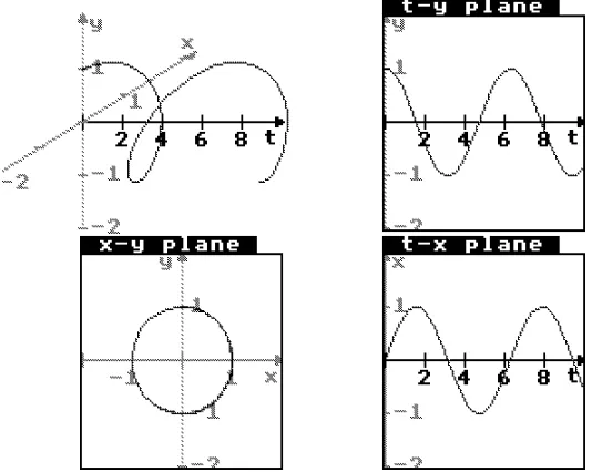
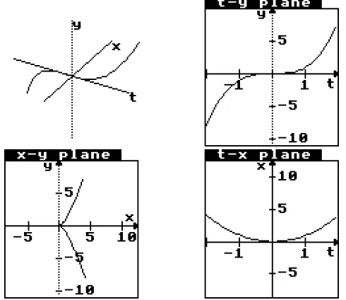
Figure 2 has been drawn with the Parametric Analyser2, a piece of software designed for the new SMP 16-19 A-level. It offers up to four windows, three coordinate planes showing the projected graphs onto the t-x, t-y, x-y planes, and a 3D picture of the graph in t-x-y space. The 3D picture in the top left hand corner, of figure 2 shows the t-y plane as an exact replica of the vertical t-y plane and the x-axis simply drawn at an angle into the plane. This can be swapped for a second projection (as in figure 3) as proper 3-dimensional view seen from any angle chosen by the user. In particular it can be rotated to give each of the three coordinate views. The action of rotating the graph gives a powerful illusion of depth to visualize the curve in three dimensional space instead of just a flat picture.

2. Visual meaning for a differential

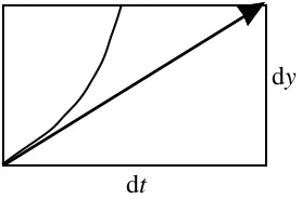
The notation is appropriate because the projection of the curve and its tangent onto a coordinate plane looks like figure 6. The diagonal of the box in this picture is projected onto the tangent to the curve in the t-y plane, and the sides of the box are dt and dy. The gradient of the tangent is then dy/dt.

dt

dy

figure 6: the projection of a tangent vector

This is exactly the definition of dt and dy given by Leibniz3 in his very first publication on the calculus. But it is one that has been neglected and misrepresented, particularly in Britain, over the last three hundred years.

In this interpretation, the lengths dt, dx, dy are differentials. They are simply the components of the tangent vector.

In the t-y plane the projection graph has an equation y=y(t). The derivative at the point (t,y) is the gradient of the tangent:

so that the derivative is expressed as a ratio of differentials. This has the advantage that the gradient of a parametric curve can be expressed as:

dy dx =

dy dt

/

dx dt

where the quantities involved are just the sides of a box in three dimensional space.

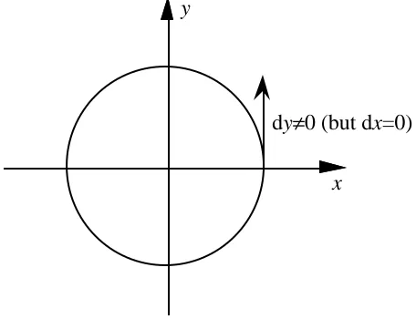
Note that, in this expression, dt can be chosen arbitrarily, and then dx and dy are defined by dx=x'(t)dt, dy=y'(t)dt, so it may happen that dx=0. But in this case, provided that dy≠0, all this means is that the tangent in the x-y plane is vertical. (Figure 7.)

x y

dy≠0 (but dx=0)

figure 7: a vertical tangent

3. Composite Functions

When I first started working with SMP on the calculus I was asked how it might be possible to give a visual interpretation of the composite of two functions and how to handle the chain rule. If we stay riveted to pictures in two dimensions this is difficult, but there is a natural interpretation in three. Given functions f:A→B and g:B→C, where A, B, C are subsets of the real numbers, we can draw a graph of f:A→B as a subset of points (x,f(x)) in AxB and g:B→C as a subset of points (x,f(x)) in BxC. The graph of fg:A→C is a subset of points in AxC. A logical way to represent f, g and gf all together is as a subset of AxBxC, using points (x,f(x),gf(x)).

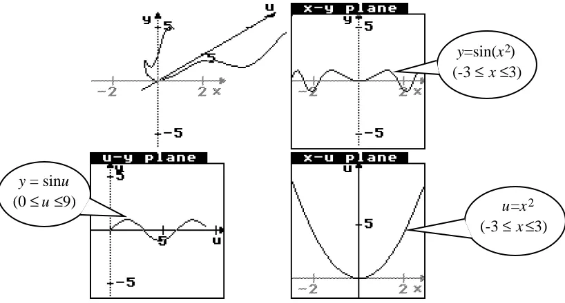
It came to me as a surprise to see that a geometrical representation of a composite of two functions can be viewed as a special case of a parametric function. Writing f and g as y=f(u), u=g(x), we obtain a parametric graph: y=f(g(x)), u=g(x), where y and u are now both functions of x. Figure 8 uses the Parametric Analyser to show the set-up

u=x2, y=sinu (=sin(x2))

in four different windows: the x-u plane in the bottom right corner, with u=x2, the u-y plane in the bottom left corner, with y=sinu, and the x-y plane in the top right, with y=sin(x2). Each of these is a projection of the curve in three dimensions in which u=x2 and y=sin(x2).

u=x

(-3 ≤ x ≤3)

2

y = sinu

(0 ≤ u ≤9)

y=sin(x )

(-3 ≤ x ≤3)

2

figure 8: a composite function seen parametrically

The only limitation is that the domain of the second function g is restricted to the image of the first function f. In the picture f has domain [-3,3], so f(x)=x2 _{has image [0,9],} and the picture restricts g to domain [0,9].

Seen as a static picture in a book this may be quite difficult to visualize, but turning the three dimensional graph around gives a sensation of space, making it easier to visualize as a three dimensional object.

Just as in the parametric case, the tangent to the curve has components dx, du, dy in directions x, u, y and the chain rule for differentiation becomes:

dy dx =

dy du

du dx

There is a well-known difficulty in this interpretation. The differential dx can be given any (non-zero) value, and then du is defined by du=u'(x) dx. If u'(x)=0 then du=0, so it cannot be used in the equation, let alone cancelled. In this case, if y'(u) is defined (as a finite value), then dy = y'(u)dx = 0. Combining this with dx≠0 gives _{dx = 0. So the}dy equation (representing the numerical values of the derivatives) is still true because both sides are zero.

It was interesting to see the reaction of various mathematicians to the idea of representing a composition of real functions as a graph in three dimensions. One said that he thought that this was the worst idea he had ever known me to have. He did not wish his students to visualize a composite function as a special case of a parametric function. He wanted to see the composite given by following one function after the other. I agree with him. But the logic of seeing a function (which is fundamentally a process relating each x in the domain to a unique f(x) in the range) as a graph (which is fundamentally a static object in the coordinate plane) has, as its logical conclusion, the visualization of a composite as an object embedded in three space.

A second reaction, quite reasonable, is that it is often hard to visualize the spatial depth of graphs in three dimensions when they are represented on a two-dimensional screen. This I agree with absolutely. For three years I have been trying to see the parametric graph x=t2_{, y=t}3 _{as a curve in space, which looks like a quadratic one way, a cubic} another and a semi-cubical parabola from a third viewpoint. (Figure 9).

figure 9: A parametrized semi-cubical parabola in three dimensions

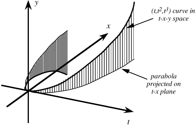
When this paper was refereed for publication one of the referees suggested that it is possible to “see” the graph (t, t2_{, t}3_{) in 3-dimensional (t, x, y) space. The perceptive} suggestion was to shade in the surface x=t2 _{with vertical lines and to draw the graph of} y=t3 on this surface (figure 10). Looking down the y-axis onto the t-x plane from above reveals x=t2_{, looking horizontally along the x-axis onto the projection on the} vertical t-y plane reveals the projected curve y=t3_{, and projecting on the vertical x-y} plane looking along the t-axis shows the parametric curve x3_=y2_.

t

x

y

parabola projected on

t-x plane

(t,t2,t3) curve in t-x-y space

figure 10 : visualising the semi-cubical parabola in 3-space

This gives visual support which helps to add depth to the picture to see the curve in space and its projections onto the axes. This would become even easier given software which allows the picture to be pulled around to see it moving and give a greater illusion of three dimensions on a two-dimensional screen. But it remains difficult to visualise more general curves in 3-space and fairly impossible in higher dimensions. What matters in the calculus is the generic mental image captured in figures 3 and 5 of a tangent to a curve as the diagonal of a box with the differentials as the components of the tangent vector.

x y

y =x2 3

figure 11: a semi-cubical parabola

Most mathematicians I know claim the tangent is the x-axis. I remember being asked to prove this in an examination. But a large number of students claim it is the y-axis, because this “touches the graph at the origin and does not cross it”4

.

The software which drew figure 9 allows the numerical tangent to the curve in three space to be drawn and to step along the curve. Only when I saw this in action did I see what I should have seen all along. If the tangent to the curve in three space is drawn a fixed length, its projection onto any of the three coordinate planes will vary depending on the angle it makes with the plane. The three-dimensional curve always has a tangent. But at the origin it points along the t-axis. Projected onto the x-y plane the tangent in this plane has zero length because it is pointing at right-angles to the plane. Of course it does. The tangent in the (x,y) plane considered as a function of t is the derivative of (t2_{, t}3_{), and is (2t, 3t}2_{), so when t=0, it is (0,0). It is only when the semi-cubical} parabola is seen as the projection of a smooth curve onto the x-y plane that the truth of the tangent at the origin becomes apparent. In the x-y plane it has zero length and does not point in any preferred direction.

4. “Implicit Functions”

form y = + 1–x2 _{, for y<0 it can be y = – 1–x}2 _{, for x>0 it is x = + 1–y}2 _{, and} for x<0 it is x = – 1–y2 _.

Thus it seems that all the “implicit functions” met in the calculus may be locally parametrized. If they cannot then the graph cannot be a curve and no derivative can be calculated. I would go further to conjecture that every “implicit function” met in A-level can be globally represented as a parametric function x=x(t), y=y(t), where the variable t has been eliminated from the relationship. In most cases found in sixth form text books this can be done using the length of the curve as the parameter. For instance, the circle given by x2_+y2_{=1 can be parametrised as x=cost, y=sint for 0}≤_t≤₂π_{. Thus, the} equation

x(t)2_+y(t)2₌₁

really represents a curve in three dimensional (t,x,y) space with tangent vector that can be found by differentiating with respect to t to give

2x dx_{dt + 2y} dy_{dt = 0.}

Of course, the dx, dy, dt have meanings as related lengths (where dt≠0) and we get

2x dx + 2y dy = 0,

or

dy

dx = –x/y.

The differential equation x dx = –y dy has meaning for all values of x, y, even when y=0, for here, if dx ≠ 0, then the tangent vector is simply vertical (as shown earlier in figure 7).

5. Partial Derivatives

The reader may wish to think how these visual ideas relate to functions of more than one variable, say z = f(x,y). In Supergraph5,6

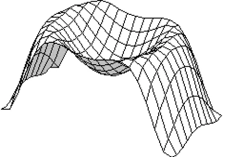
these graphs are drawn using lines in the direction x=constant and y=constant to give a rectangular grid on the surface (figure 11). The two dimensional equivalent to local straightness is local flatness, which means that any small part of the surface approximates to a plane. It can therefore be approximated by a rectangular tiling where each flat tile is suitably small to give a good approximation to the surface. In practice a fairly good representation can be obtained with a comparatively small number of tiles (figure 12 has a 10 by 20 array of rectangles).

figure 12: A (locally flat) surface in three dimensions

One way of imagining the notion of partial derivatives is to look along the lines x=constant and y=constant. When y is constant, say y=y0, then z is a function of x, z=f(x,y0). Traditionally the gradient of this graph is denoted by ∂z/∂x. But this notation is misleading in that the corresponding notation for the gradient when x is constant is

∂z/∂y and, both cannot be thought of as quotients for increments ∂x and ∂y because the value of ∂z is not the same in each case.

Therefore we need a new notation. For fixed y, consider the limit as h→0 of f(x+h,y)-f(x,y)

h

which is normally denoted by ∂z/∂x.

dx

dzx

x z

x

z=f(x,y) for y=constant as a function of x

figure 13 : cross-section of the surface z=f(x,y) through a plane y=constant.

Likewise, taking a cross-section for fixed x gives z=f(x,y) as a function of y and we denote by dy any increment in y and by dzy the corresponding increment to the tangent

line. Viewed in three dimensions this gives figure 14.

dx

dzx

dzy

dzx+dzy

(x,y) z

(x+dx, y+dy)

dx

dy

(x,y,z)

x

y

tangent plane at (x,y,z)

surface

dz = dzx

dy

x

y z

It shows the plane y=constant at the front with x increment dx and increment dzx up to

the tangent plane. Meanwhile, the plane x=constant has y increment dy and increment dzy up to the tangent plane. The vertical distance from the point in the tangent plane

vertically above (x,y) to the point in the tangent plane vertically above (x+dx, y+dy) is

dzx+dzy.

This is usually called the total differential dz

and

dz = dzx+dzy.

If one so desires this can be rewritten as

dz = dz_{dx dx +} x dz_{dy dy}y

where the expressions dz_{dx ,} x dz_{dy are both partial derivatives, now expressed as}y quotients of lengths.

This is a whole lot more meaningful than the usual equation:

dz = ∂_∂z_{x dx +} ∂_∂z_{y dy}

where the partial derivatives are not quotients because the ∂z represent different concepts in the two expressions.

6. Conclusion

References

1. Tall D. O. ,1985 : “Tangents and the Leibniz notation”, Mathematics Teaching, 112 48-52.

2. Tall D. O., 1991: Real Functions & Graphs, (software for the BBC, Nimbus & Archimedes), C.U.P., Cambridge.

3. Leibniz G.W., 1684 : “Nova methodus pro maximis et minimis, itemque tangentibus, qua nec fractas, nec irrationales quantitates moratur, & sinulare pro illis calculi genus ”, Acta Eruditorum, 467-473.

4. Vinner S., 1982: “Conflicts between definitions and intuitions – the case of the tangent”, Proceedings of the 6th International Conference of P.M.E., Antwerp, 24-28.

5. Tall D. O., 1986: Supergraph, (software for the BBC computer, Nimbus & Archimedes), Glentop Press, London.