Mathematical Model and Computational Studies of
Discrete Dislocation Dynamics
Miroslav Kol´aˇr, Michal Beneˇs, Daniel ˇSevˇcoviˇc, Jan Kratochv´ıl
Abstract—This contribution deals with the numerical simu-lation of dislocation dynamics, which is a topic belonging to the field of solid state physics. Dislocations are modelled as line defects in crystalline lattice causing the disturbance of the regularity of the crystallographic arrangement of atoms. From the mathematical point of view, dislocations are defined as smooth closed or open planar curves, which evolve in time, and their motion is driven by the equation for the mean curvature flow stating that the normal velocity is proportional to the mean curvature and the sum of all acting force terms. In this paper, we describe the family of evolving curves by the parametric approach, and the system of PDEs arising from the mean curvature motion law is solved by semi-implicit scheme with spatial discretization based on the flowing finite volume method. Additionally, we enhance the performance and the numerical stability of the algorithm by adding a tangential term to the motion law. The presented results of numerical simulations contain the motion of a single dislocation in the PSB channel and the motion and mutual interaction of two dislocation curves in the PSB channel.
Index Terms—Dislocations, mean curvature flow, tangential redistribution, flowing finite volume method, PSB channel.
I. INTRODUCTION
A
LL real crystals contain some imperfections, which locally disturb the regular arrangements of the atoms. These imperfections may have point, line, surface or vol-ume character and they occur in nanoscale. However, their presence can significantly influence the physical and me-chanical properties of crystalline solids. In this paper, we are concerned with dislocations, which are line defects of the crystalline lattice. They act in such a way that the crystallographic arrangement of atoms is disturbed along a so called dislocation line. Even though the dislocation theory concerns the solid state physics and material sciences, it can be considered relatively young (compared to other physical disciplines in macro scale). Throughout the last century presence of dislocations has been experimentally verified and the theoretical framework, which is extensively discussed in the literature (see, e.g., [1], [2]) has been developed.From the mathematical point of view, dislocations can be represented as closed curves (acting inside the crystal) or open curves (ending on a surface of the crystal), which
Manuscript received December 23, 2013; revised August 16, 2014. This work has been supported by the grant Two scales discrete-continuum approach to dislocation dynamics, project No. P108/12/1463 of the Grant Agency of the Czech Republic and VEGA grant 1/0747/12 (DS).
M. Kol´aˇr and M. Beneˇs are with the Department of Mathematics, Faculty of Nuclear Sciences and Physical Engineering, Czech Technical University in Prague, e-mail: [email protected] (corresponding author), [email protected], respectively.
D. ˇSevˇcoviˇc is with the Department of Applied Mathematics and Statistics, Comenius University, Bratislava, Slovak Republic, e-mail: [email protected].
J. Kratochv´ıl is with the Department of Physics, Faculty of Civil Engineer-ing, Czech Technical University in Prague, e-mail: [email protected].
can, under certain physical conditions, evolve in time and space and even interact with each other. At certain physical conditions, e.g., at low homologous temperature, the motion is only two-dimensional and dislocations can move only along the so called slip planes, i.e., some crystallographic planes with the highest density of atoms. We describe the motion by means of the mean curvature flow and the parametric approach [17], [10] and enhance the model by adding the curvature adjusted tangential redistribution [14], which was originally proposed for closed curves only. Our contribution is in modifying the redistribution algorithm for open dislocation curves.
We investigate the motion and interaction of dislocations in PSB channel [1], [2], [8] and present novel numerical results for evolution of open dislocation curves computed by means of curvature adjusted tangential redistribution.
II. MATHEMATICALMODEL
Generally, to model a motion of curves or interfaces, the equation for the mean curvature flow is usually investigated. Its basic dimensionless form is
normal velocity=curvature+force. (1) Taking into account the dislocation dynamics, more precise description preserving physical units of measurement is given by equation (2) below.
There are several approaches to treat equation (1). Very popular methods come from the family of interface capturing approaches, such as the phase-field method [5], [7] or the level set method [3], [4], [6]. It is often referred, that their main advantage is their ability to deal with topological changes, such as merging or splitting, with almost no difficul-ties. However, when applying such approaches to problems of discrete dislocation dynamics (where evolution in long time interval and evaluations of relatively complex spatially-dependent terms are often required), one experiences some difficulties mainly in the computational cost. For instance, in the case of a planar curve, which is, in fact, a one-dimensional object, it is required to solve a two-one-dimensional problem, and thus the interface capturing methods are too slow.
A fast method for evolving curves is provided by the parametric approach [8], on which we also focus in this contribution. It needs to be mentioned, that the parametric approach cannot deal with topological changes on its own. However, separate algorithms to deal with such a task can be developed [17].
It shows that the mathematical theory of evolving curves is very useful framework to model the motion of dislocations (see [8], [10]). In this paper, we investigate their evolution
IAENG International Journal of Applied Mathematics, 45:3, IJAM_45_3_05
governed by the mean curvature flow (1) in the following form
Bv=T κ+F. (2)
Here v is the normal velocity (considering outer normal vector),κdenotes the mean curvature of the curveΓ = Γt,
which is a closed or an open curve in a plane. The F
is the forcing term. The terms B and T are just physical parameters, which we discuss in the next section along with the particular choice of the force F.
Our goal is to find a family {Γt : t ∈ [0, Tmax]} of
closed or open curves in the plane, whose normal velocity is proportional to the mean curvature and the force, i.e., satisfies the equation for the mean curvature flow (2).
As already mentioned, in this contribution, we treat equa-tion (2) by means of the parametric (also referred as the direct or the Lagrangian) approach as in [8]. There are two common ways in which the planar curveΓtcan be parametrized. The first one is called fixed domain parametrization, where we introduce a parameterubelonging to a fixed interval, which is independent of time, e.g., u∈[0,1]. Then the family of planar curves is given as the following set
Γt={X~(u, t) = (X1(u, t), X2(u, t)) :u∈Iu}.
Here the curve Γt is described by the space and time dependent vector mapping
~
X :Iu×It→R2,
where Iu = [0,1] is the fixed interval for the parameter u
andIt= [0, T]is the time interval.
The second type of parametrization of a planar curve is the so called arc-length parametrization which is also represented by a mappingX~(s, t), where the parametersis bounded by the actual length of the curve at time t. Denoting Lt the actual length of the curve at timet, the family of the planar curves is given as
Γt={X~(s, t) = (X1(s, t), X2(s, t)) :s∈[0, Lt]},
whereX~ : [0, Lt]×It→
R2.
Denoting by g the quantity g=|∂uX~|>0 as the local
length, the relation between the arc-length parametrization and the fixed domain parametrization reads as ds=gdu
and the variable transformation for a quantity ϕ is given by∂uϕ=g∂sϕ.
In our paper the numerical approach is based on the finite volume method. It is therefore natural to treat equation (2) by means of the arc-length parametrization.
We define the unit tangential vector ~t to the curve as
~t = ∂uX/|∂u~ X|~ = ∂sX~. The outer unit normal vector ~n
is defined as ~n = ∂sX~⊥, where ⊥ is the symbol of per-pendicularity and det(~n, ~t) = 1holds. Both parametrizations are oriented counterclockwise. Note that X~ =X~(u, t) and
~
X =X~(s, t)are different mappings with the same range. In this paper, we intentionally use the same symbolX~ for both mappings to simplify the text. Time derivatives in equations (3), (4), (9) are taken in sense of arc-length parametrization, i.e.,∂tX~(s, t).
The normal velocity v is the time derivative of X~(t, s) projected into the normal direction, i.e., v=∂tX~ ·∂sX~⊥. According to the Frenet formulae, one can derive the curva-ture asκ=∂s~t·∂sX~⊥=∂ssX~ ·∂sX~⊥. Note the curvature
of the unit circle is−1. Then equation (2) can be written as
B∂tX~ ·∂sX~⊥=T ∂ssX~ ·∂sX~⊥+F(X~), (3) provided that the unknown mappingX~ satisfies the paramet-ric equation
B∂tX~ =T ∂ssX~ +F(X~)∂sX~⊥. (4) Equation (4) is complemented with the initial condition
~
X|t=0=Xini~
and either the periodic boundary conditions for closed curves or fixed ends boundary conditions for open curves
~
X|s=0=X~A, ~X|s=Lt =X~B.
III. PHYSICAL MODELING OF EXTERNAL FORCES FOR DISLOCATION DYNAMICS
The aim of this section is to recall the main idea of phys-ical modelling of external forces. Recalling the governing equation (2) and its parametric form (4), we want to describe the physical parameters of the proposed model of evolving dislocations. HereB is the drag coefficient and the symbol
T denotes the line tension [1], which is, basically, the weak anisotropic term causing straightening of the dislocation curve. In this paper, we consider the simplified isotropic model, where the line tension is approximated as follows
T ≈E(e)(1 +ν). (5)
The constants E(e) and ν are the dislocation edge energy [1] and the Poisson ratio, respectively. The particular choice of the model parameters is presented in Table I. In the following, we denote by b the magnitude of the Burgers vector~b= (b,0,0) and identify the slip plane with thexz -plane.
The termF is the sum of all outer force terms acting on the curveΓtin the normal direction, i.e.,
• forceFapp=bτappcaused by the resolved shear stress
τapp applied on the crystal,
• force Fwall = bτwall caused by the stress τwall from the walls of the PSB ([1], [2]) channel,
• force Fint = bτint caused by the mutual interaction stressτintbetween the dislocations in the PSB channel, • force Ff r = bτf r caused by the crystalline lattice
resistance. This friction force slows down the movement of the dislocation, and therefore it has to be subtracted from the total force contribution.
Then the sum of all outer forces is the following
F =Fapp+Fwall+Fint−Ff r. (6)
The last term which has to be taken into the account is the forceFself =bτself, where the stress fieldτself is generated by the dislocation itself. In [9] Kratochv´ıl and Sedl´aˇcek proved that the dislocation self force is proportional to the curvature of the corresponding dislocation curve. The term
T κin (2) approximates the self force of the dislocation.
IAENG International Journal of Applied Mathematics, 45:3, IJAM_45_3_05
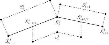
Fig. 1. Schematic illustration of the PSB channel with walls simulated by dipoles. Dislocation (thick black line) evolves inxzplane (slip plane).
A. Wall interaction
The motion of a dislocation itself is considered within the so called PSB (persistent slip band) channel [1], [2], [8]. Generally, it is a pattern consisting of areas with high density of dislocations (channel walls) and low densities of dislocations (channel itself). This structure usually arises from a cyclic loading of a crystal. When a dislocation moves in the PSB channel, it interacts with the dipolar loops created by other closed dislocation curves inside the crystal. In particular, the clustered dipolar loops create the channel walls. This interaction is usually simulated as elastic fields of infinite edge dipoles in the channel walls, which act like a potential wells generated by the dipoles.
The situation is schematically illustrated in Figure 1. The dislocations D1 andD2 form a dipole in the left wall and the dislocationsD3 andD4 form a dipole in the right wall. Its strength is given by the mutual distance hdip. All the four dislocations are ydip under or above the slip plane and the parameter ddiprepresents the distance from the channel walls, which are at a distance dc.
According to [18], the resolved shear stress in the slip plane produced by an edge dipole approximating the dislo-cations D1 andD2 is given as
τwall(1) = Gb 2π
1 1−ν
x1(x2 1−y21) (x21+y21)2 −
x2(x2 2−y22) (x22+y22)2
,
wherex1andy1are the coordinates of a point in the channel relative to the dislocation D1. Analogously x2 and y2 are coordinates of the same point related to the dislocationD2. Because of the symmetry of the channel, interaction is only considered in the direction of the x-axis. Here, G denotes just the shear modulus and ν stands for the Poisson ratio (see Table I).
Similarly, the same considerations can be done for a dipole approximating the dislocations D3 and D4. In our simulations, we consider the dislocation curve Γ to belong to a slip plane y= 0within a channel with its mid point at
x= 0. Then, for a given point(x,0, z)we have
x1,3=±x+dc/2 +ddip+hdip, y1,3=ydip,
x2,4=±x+dc/2 +ddip, y2,4=−ydip, where the parameters of the channel are in Table I.
Then the formula for the resolved shear stress produced by both walls reads as follows
τwall=τwall(1) +τwall(2)
-0.02 -0.015 -0.01 -0.005 0 0.005
-600 -400 -200 0 200 400 600
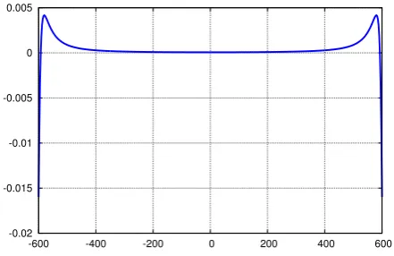
Fig. 2. Wall force function, the x-axis is in nanometers, the y-axis is in Newtons.
and the force generated by the channel walls reads as
Fwall=bτwall.
It follows that the channel wall force Fwall =Fwall(x) =
Fwall(X1)and acts in thex-axis of the channel. The graph is depicted in Figure 2.
B. Dislocation interaction
We consider the dislocation motion to be influenced by interactions with other dislocations. Since we approximate the dislocations as polygonal curves (details can be found in Section 4), all force interactions are sums of contributions of straight dislocation segments.
To solve the problem of dislocation interactions, one needs to determine the stress tensor field τint = (τint)i,j =
(τint(X~))i,j at a position X~ from a straight segment AB
of a dislocation. This problem was theoretically solved by Devincre in [11]. There exists a general formula providing the 3D stress tensor field τA(X~) = (τA
ij)(X~) at a position ~
X generated by the dislocation half line from the pointA~ to infinity and reads as
τijA= G
4π
1
R(U+R)
"
(~b×Y~)itj+ (~b×Y~)jti
− 1
1−ν((~b×~t)iYj+ (~b×~t)jYi) −~b·(~%×~t)
1−ν
δij+titj+
%i%j(2 +U/R)
R(U+R) +(%itj+%jti+U titj)(U+R)
R2
#
,
(7)
where ~t is the unit tangential vector to the dislocation segment, R is the magnitude of the vector R~ = X~ −A~,
~
% = R~ −U~t is the distance vector from the dislocation and U = R~ ·~t is the projection of the vector R~ to the dislocation segment.Yi andYj are components of the vector
~
Y =R~+R~tandδijis the Kronecker symbol. Here·denotes the scalar product and the symbol × stands for the cross product.
The stress tensor generated by one straight dislocation segment AB is given as the difference of the tensors τA
IAENG International Journal of Applied Mathematics, 45:3, IJAM_45_3_05
[image:3.595.318.539.65.208.2]andτB
(τint(X~))ij =τijA−τ B ij.
Then the total stress is given as the sum of stress contribu-tions from all the segments of the dislocation.
The force acting on the dislocation exposed to the stress field τint is given by Peach-Koehler formula [12], which reads as
~
Fint= (τint~b)×~t. (8)
We consider the Burgers vector~b= (b,0,0) parallel to the
x-axis and the slip plane y = 0. The unit tangential vector
~tis of the form~t= (t1,0, t3)and the unit normal vector is
~
n= (t3,0,−t1). Then the vectorial forceF~int given by (8)
is
~
Fint= (τint~b)×~t=b(τ12t3, τ13t1−τ11t3,−τ12t1). Hence the normal component of the interaction force is
Fint=F~int·~n=b(τ12t23+τ12t21) =bτ12.
According to these formulas and the above settings of the model it is clear that only the component τ12 of the stress tensor is to be computed. Since we investigate the interaction of dislocations in parallel slip planes in this paper, it is clear that the singularity, which appears in (7) atR= 0is avoided.
IV. NUMERICALALGORITHM
Our approach is based on the numerical scheme pro-posed by ˇSevˇcoviˇc and Yazaki in [14], [15] with spatial discretization by means of the flowing finite volume method. Discretization in time then leads to a semi-implicit scheme. The scheme was originally proposed for evolution of closed curves. Here we extended it to the case of open curves. We show how to enhance the governing equation and design a tangential redistribution for open curves, which will be mentioned below.
A. Tangential Redistribution
Gage and Epstein showed (see [13], Proposition 2.4) that when tracking a curve motion, the tangential terms do not affect the curve shape. Hence, for the analytical purposes, it is sufficient to take into the account only the terms in the nor-mal direction to the curve. However, numerical experiments show that the parametric equations (4) are not appropriate for numerical computation. Since the curve is discretized by a certain number of grid points (except the perfectly symmetric and uniform cases with constant curvature, like a shrinking circle), we can observe that during the time evolution, the grid points accumulate in certain parts of the curve, while they become sparse elsewhere. This phenomenon is not desirable particularly in long time simulations, where this non-uniform distribution of grid points can cause increasing numerical error. One possible way to overcome this problem is to employ some kind of tangential redistribution, i.e., to complement equation (4) with a tangential term
B∂tX~ =T(∂ssX~ +α∂sX~) +F(X, t~ )∂sX~⊥. (9) The redistribution coefficient α is a (possibly nonlocal) function of the position vector X~ and its first and second derivative. Generally, the tangential terms move the dis-cretization points along the curve without affecting its shape.
If correctly chosen, the numerical algorithm is more stable and has higher accuracy. On the other hand, wrong choice of tangential terms can lead to numerical errors, and in the worst case, to the failure of the algorithm.
Basically, the further modifications lead to the form of (4) with a local tangential redistribution, originally proposed for closed curves, by Deckelnick and Dziuk in [19]. Differenti-ating the∂ssX~, we obtain
∂ssX~ = 1
|∂uX|~ ∂u(∂s ~
X) = 1
|∂uX|~ ∂u ∂uX~
|∂uX~| !
= ∂uu
~ X
|∂uX|~ 2
−∂uX~ ·∂uuX~ |∂uX|~ 3
∂uX~
|∂uX|~ ,
Then, the following equation
∂tX~ = ∂uuX~
|∂uX~|2
+F∂uX~ ⊥
|∂uX|~
already contains a local tangential term with redistribution coefficientαloc:
αloc=
∂uX~ ·∂uuX~
|∂uX|~ 3 .
However, numerical experiments show that this local redis-tribution property is not strong enough to prevent the grid points from accumulating in certain segments of the curve. Thus in (9), the local tangential term αloc∂sX~ is replaced
by a general, possibly nonlocal tangential termα∂sX~.
The problem of tangential redistribution has been ex-tensively studied. We use the curvature adjusted tangential redistribution originally proposed by ˇSevˇcoviˇc and Yazaki for closed curves in [14], where one can also find a brief overview and a critical discussion of the redistribution meth-ods. In this paper, we adapted the original algorithm for evolution equation (9) and developed a modification suitable for open curves.
According to [14], the redistribution coefficient has been proposed as the solution of the following problem
∂s(ϕ(κ)α) =H,where (10)
H =f− ϕ(κ)
hϕ(κ)ihfi+ω Lt
|∂uX|~
hϕ(κ)i −ϕ(κ)
!
.
The quantity Lt is the curve length at time t and the parameter ω is a given positive constant. The other factors in the problem (10) are as follows
ϕ(κ) =1−ε+εp1−ε+κ2ε2,
f =ϕ(κ)κ(T κ+F)
−ϕ0(κ)(∂ss(T κ+F) +κ2(T κ+F)), hϕ(·, t)i=1
Lt Z
Γt
ϕ(s, t)ds.
The functionϕ(κ)plays an important role because it controls the redistribution of the grid points. The special choice of
ε= 0, i.e.,ϕ(k) = 1produces the uniform redistribution and asymptotically uniform redistribution forε >0. The choice of ε = 1, i.e., the function ϕ = |κ| was proposed for the crystalline curvature flow (see [16]). Choosing ε ∈ (0,1), we obtain the curvature adjusted redistribution as in [14], which takes into account the shape of the curve. The ratio
IAENG International Journal of Applied Mathematics, 45:3, IJAM_45_3_05
Fig. 3. Spatial discretization by flowing finite volume method.
ϕ(κ)/hϕ(κ)i was used by ˇSevˇcoviˇc and Yazaki to capture deviations of|κ|and hence to design the curvature adjusted tangential term α. Detail of their research can be found in [14].
The redistribution coefficient α=α(s, t) is uniquely (up to an additive constant) determined from (10). In the case of closed curves, ˇSevˇcoviˇc and Yazaki imposed renormalization constraint
hα(·, t)i= 0 (11)
to determineαuniquely. In the case of open curves, we have to ensure
α(0, t) =α(Lt, t) = 0 (12) for all t >0. Clearly, as ϕ(κ(Lt))>0, settingα(0, t) = 0
and integrating (10) over the curve Γt with respect to the
arc-length yields
ϕ(κ)α(s, t)|s=Lt =ϕ(κ)α(s, t)|s=0+
Z
Γt
H(s)ds= 0,
(13) because one can see that
Z
Γt
Hds=ω(Lthϕi −Lthϕi) = 0
and the uniqueness condition (12) holds.
B. Finite volume method
Given an initial N-sided polygonal curve P0 =∪N i=1Si0
with vertices X~i0 approximating the initial curve Γ0, we find a family of N-sided polygonal curves {Pj}j
=1,2,...
with vertices X~ij, where Pj = ∪N i=1S
j
i for i-th edge Sij = [X~ij−1, ~Xij], which represents the control volume. The polygonPj is constructed as an approximation ofΓt at the
j-th time level tj = jτ and the updated polygon Pj+1 is determined from thePj at the previous time step by solving the systems of PDEs (9) and (10).
We consider thei-th dual volume νij as the following set
νij = [X~ij−1/2, ~Xij]∪[X~ij, ~Xij+1/2],
where the quantitiesX~ij±1/2are the averages on the primary
volumes Sij+1 andSij, respectively
~
Xij−1/2=
~
Xij−1+X~ij
2 ,
~
Xij+1/2=
~
Xij+X~ij+1
2 .
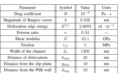
Here, notice that the symbol ν stands for the Poisson ratio (see Table I), whereas the symbolνij denotes the particular dual volume. The scheme of the discretization is shown in Figure 3.
Besides theX~ij, we introduce the following discrete quan-tities: αji,κji, and dji =|Sji| with their dual values defined in the same way asX~ij±1/2
αji−1/2= α
j i−1+α
j i
2 , α
j i+1/2=
αij+αji+1
2 ,
κji−1/2= κ
j i−1+κ
j i
2 , κ
j i+1/2=
κji+κji+1
2 ,
dji−1/2= d
j i−1+d
j i
2 , d
j i+1/2=
dji +dji+1
2 .
These quantities are naturally classified into two categories as follows:
• κji anddji are constant on the i-th edge Sij and satisfy the duality condition, i.e., the dual values κji+1/2 and
dji+1/2 are constant value on the corresponding dual
volumeνij.
• αji andX~ij are defined on the i-th vertexX~ij and take constant value on the i-th dual volume νji, whereas the dual value αi−1/2 remains constant on the primary volumeSij.
We denote Lj = PN i=1d
j
i as the total length of P j and
hGji=PN i=1G
j id
j
i as the mean value of a quantityG jover
Pj.
At first, the values fordji andκji are computed from the previous known data according to the following formulas, where the discrete curvature is approximated in agreement with [14], [17].
1) ~pji =X~ij−X~ij−1, 2) dji =|~pji|, 3) κji = 1
2djisgn det(~p j i−1, ~p
j i+1)
arccos
~ pji−1·~pji+1
dji−1dji+1
.
Then the redistribution coefficients αi are computed via relations (16) and (15) below.
Finally, the position vector X~ij is computed by solving (18).
C. Discretization of the tangential velocity equation
In [14] ˇSevˇcoviˇc and Yazaki proposed the following al-gorithm for closed curves, where all quantities X~ij, αji,κji
anddji satisfy the periodic boundary conditions. There is a modification for open curves with fixed ends, which we will mention at the end of this section.
We integrate equation (10) over the control volumeSi = [Xi~ −1, ~Xi]with respect to the arc-length parameters
Z X~i
~ Xi−1
∂s(ϕα)ds= Z X~i
~ Xi−1
fds− Z X~i
~ Xi−1
ϕhfi hϕi ds
+
Z X~i
~ Xi−1
ω Lt
g hϕi −ϕ
ds,
(14)
where
Z X~i
~ Xi−1
fds=
Z X~i
~ Xi−1
ϕ(κ)κ(T κ+F)ds
− Z X~i
~ Xi−1
ϕ0(κ)(∂ss(T κ+F) +κ2(T κ+F))ds.
Here we use the following finite differences to evaluate the second derivative of the curvature and the force. Note that
IAENG International Journal of Applied Mathematics, 45:3, IJAM_45_3_05
the curvature remains constant on the control volume Sij, while the force term is defined pointwise, or more precisely at each vertexX~ij. We have
(∂ssκ)(X~ij−1/2) = 1
dji[∂sκ] ~ Xij
~ Xij−1
= 1
dji
κji+1−κji di+1/2
−κ j i −κ
j i−1
di−1/2
!
,
(∂ssF)(X~ij−1/2) = 1
dji[∂sF] ~ Xji
~ Xji−1
= 1
dji
Fij+1−Fij
dji+1 −
Fij−Fij−1
dji !
.
By taking averaged spatial values in (14), we obtain the following system of finite differences equations for the tangential velocity. Note that from direct calculation
RX~i
~
Xi−1(1/g)ds = 1/N due to
~
Xi =X~(ui), ds =gdu and
ui+1−ui= 1/N.
ϕ(κji+1/2)αji+1−ϕ(κij−1/2)αij−+11 =ψji, (15) where
ψji =fijdji− ϕ(κ j i) hϕ(κj)ihf
jidj i +ω
Lj
Nhϕ(κ
j)i −ϕ(κj i)d
j i
is defined for the discrete quantity
fij =ϕ(κji)κjiT κji +F(X~ij−1/2)
−ϕ
0(κj i) dji T
"
κji+1−κji
dji+1/2 −
κji −κji−1
dji−1/2 #
+ F
j i+1−F
j i
dji+1 −
Fij−Fij−1
dji !
−ϕ0(κji)(κji)2(T κji+F(X~ij−1/2)).
From (15) we can obtain the following recurrent formulation
ϕ(κji+1/2)αji+1=ϕ(κj1+1/2)αj1+1+ Ψji, Ψji =
i X
k=2
ψkj.
From (11) we have hαj+1i = 0 and hence
PN
i=1d
j i+1/2α
j+1
i = 0 holds. Therefore we can ensure
the uniqueness of the solution αj+1 and set
ϕ(κj1+1/2)αj1+1=−
PN
i=2d
j i+1/2Ψ
j i/ϕ(κ
j i+1/2)
PN
i=1d
j
i+1/2/ϕ(κ
j i+1/2)
. (16)
The modification for open curves satisfying the fixed ends boundary conditions X|s~ =0 = X~A, ~X|s=Lt = X~B is just
to set αj0+1 =αjN+1 = 0, which represents zero tangential speed sinceXA~ andXB~ are fixed. For the quantitiesκji and
dji instead of periodicity, the mirroring technique is used.
D. Discretization of the equation for the position
We integrate the equation (9) over the dual volumeνiwith
respect to the arc-length parameter s
Z X~i+1/2
~ Xi−1/2
B∂tX~ds=
Z X~i+1/2
~ Xi−1/2
T ∂ssX~+αT ∂sX~+F ∂sX~⊥ds,
from which, by taking discrete time stepping and averaged values, we obtain the following equation (note that the force termF is considered constant on the dual volume νi)
Bdji+1/2(∂tX~) j+1
i =T h
∂sX~ iX~ji+1+1/2
~ Xji−+11/2
+αji+1ThX~i ~ Xij+1+1/2
~ Xij−+11/2
+FijhX~⊥i ~ X⊥,j
i+1/2
~ X⊥,j
i−1/2
.
(17)
Using the following differences ofX~ij, where the nonlinear-itiesdji are taken at the previous time level,
(∂sX~) j+1
i+1/2=
~
Xij+1+1−X~ij+1
dji+1 ,
(∂sX~) j+1
i−1/2=
~
Xij+1−X~ij−+11
dji ,
(∂tX~)ji+1=
~
Xij+1−X~ij
τ ,
the following semiimplicit linear system for the position vectorX~ij+1
−aji+1/2τ ~Xij−+11 + (1 +bji+1/2τ)X~ij+1−cij+1/2τ ~Xij+1+1
=X~ij+τF j i B
~
Xi⊥−,j1−X~⊥,j i+1
dji+1+dji
(18)
with the coefficients
aji+1/2= T
B
1
dji+1/2
1
dji − αji+1
2
!
,
cji+1/2= T
B
1
dji+1/2
1
dji+1 + αji+1
2
!
,
bij+1/2=aij+1/2+cji+1/2.
The system (18) is tridiagonal and can be easily solved by matrix factorization.
V. COMPUTATIONALRESULTS
We present results of numerical simulations of the motion of dislocations in the PSB channel. In the first study, we consider the motion of a single dislocation. Moreover, we present the results of two numerical experiments, in which we deal with the interaction of two dislocations on nearby parallel slip planes in the PSB channel. All simulations are considered under real physical settings, which are summa-rized in Table I. The values of model parameters used in numerical examples are: number of finite volumesN= 150, time stepτ =B·104/N, tangential redistribution parameters
ω = 0.1, ε = 0 (0.1 in one dislocation evolution), and approximate line tensionT =E(e)(1 +ν)(see (5)).
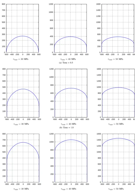
A. Single dislocation line
We consider one straight initial dislocation line with fixed endpoints in the channel walls, which is driven by the force
F=Fapp+Fwall−Ff r.
We study the influence of the various values of the applied stressτapp, which areτapp= 30,40,50 MPa, respectively.
IAENG International Journal of Applied Mathematics, 45:3, IJAM_45_3_05
TABLE I
TABLE OF PHYSICAL PARAMETERS
Parameter Symbol Value Units
Drag coefficient B 10−5 Pa·s
Magnitude of Burgers vector b 0.256 nm Dislocation edge energy E(e) 2.0693 nJ·m−1
Poisson ratio ν 0.34 —
Shear modulus G 42.1 GPa
Friction τf r 5 MPa
Width of the channel dc 1200 nm
Distance of dislocations hdip 20 nm Distance from the slip plane ydip 10 nm Distance from the PSB wall ddip 10 nm
The results are shown in Figure 4. As the dislocation evolves, it attaches to the walls of the PSB channel, while the apex of the dislocation in the center of the channel moves onward. Additionally, we can see that when the applies stress is higher, the dislocation is more straightened.
B. Interaction of two dislocations in PSB channel
We consider two straight initial dislocation lines with fixed endpoints in the channel walls, driven by the forces (6) with opposite signs. The dislocations are located on different slip plane with the distanceh.
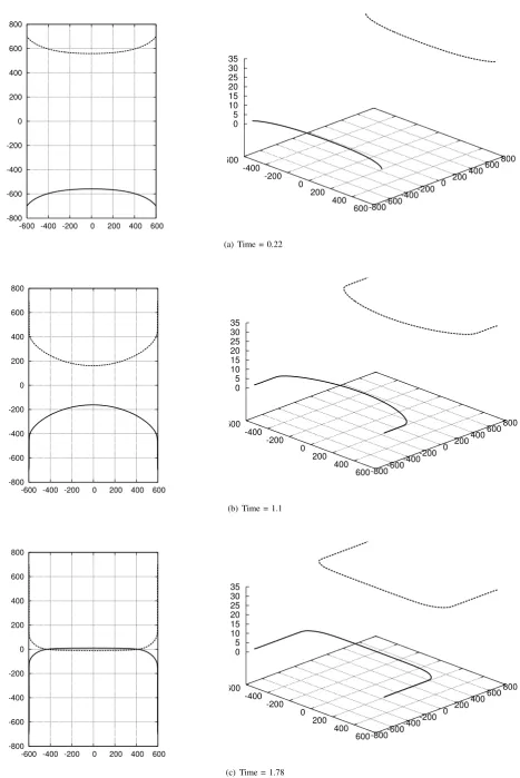
In the first experiment shown in Figure 5, the distance between the slip planes is h= 35 nm and we consider the value of the applied stress τapp = 30MPa. The interaction
force is attractive, speeds up the motion and both dislocations (solid and dashed curves) are attracted to each other. How-ever, since the distance of slip planes is relatively small, the interaction force is strong and when the dislocations overlap, the total force becomes repulsive, which stops the movement at a certain position, leaving the dislocations in a steady state. In the second experiment (see Figure 6), the mutual distance between the slip planes ish= 65nm and the value of the applied stress isτapp= 35MPa. The interaction force also attracts the dislocations. When the dislocations (solid and dashed curves) overlap, the interaction force becomes repulsive. In this case of relatively large distanceh, the force generated by channel walls and applied stress is greater than the repulsive force and the dislocations continue to glide.
VI. CONCLUSION
We have presented a mathematical and physical model of evolving curves in plane based on the parametric approach and discussed the problem of non-uniform distribution of grid points. We successfully overcame this problem by adding a curvature adjusted tangential term to the model, which has been shown to be a very useful technique for stabilizing the numerical algorithm. We presented a method for computing the redistribution coefficients by discretization of the equation for the tangential velocity by means of the flowing finite volume method and we used the very same approach to treat the motion law of evolving curves. We also modified the redistribution algorithm for evolution of open dislocation curves. We introduced a physical model of evolving dislocations and discussed the outer forces affecting the motion and the interaction of two dislocation curves,
respectively. We present novel numerical results for evolution of open dislocation curves in the PSB channel computed by means of curvature adjusted tangential redistribution. Previ-ous computational studies showed importance of tangential redistribution. In Min´arik (see [8], [10]), much simpler redistribution was implemented. Here we apply the curvature adjusted tangential redistribution which is more suitable for curve evolution problems with high variations in curvature.
ACKNOWLEDGMENT
The authors would like to express their sincere thanks to the reviewers for their valuable comments and suggestions for the improvement of this paper. We would also like to thank to Dr. Shigetoshi Yazaki for valuable discussion about the topic of tangential redistribution.
REFERENCES
[1] D. Hull and D Bacon, “Introduction to dislocations,” Butterworth-Heinemann (2001).
[2] T. Mura, “Micromechanics of Defects in Solids,” Kluwer Academic Publishers Group (Netherlands, 1987).
[3] S. A. Sethian, “Level set method and fast marching methods,” Cam-bridge University Press (CamCam-bridge, 1999).
[4] S. Osher and R. P. Fedkiw, “Level set method and dynamic implicit surfaces,”Springer (New York, 2003).
[5] M. Beneˇs, “Mathematical analysis of phase-field equations with nu-merically efficient coupling terms,”Interfaces and Free Boundaries, 3 (2001), pp. 201–221.
[6] D. Jayadevappa, S. Srinivas Kumar and D. S. Murty, “New Deformable Model Based on Level Sets for Medical Image Segmentation,”IAENG International Journal of Computer Science, 36:3 (2009), pp. 199–207. [7] T. Ohta, M. Mimura and R. Kobayashi, “Higher-dimensional localized patterns in excitable media,” Physica D: Nonlinear Phenomena, 34 (1989), pp. 115-144.
[8] M. Beneˇs, J. Kratochv´ıl, J. Kˇriˇst’an, V. Min´arik and P. Pauˇs, “A parametric simulation method for discrete dislocation dynamics,”The European Physical Journal ST, 177 (2009), pp. 177-192.
[9] J. Kratochv´ıl and R. Sedl´aˇcek, “Statistical foundation of continuum dislocation plasticity,”Physical Review B, 77 (2008), p. 134102. [10] V. Min´arik, M. Beneˇs and J. Kratochv´ıl, “Simulation of dynamical
interaction between dislocations and dipolar loops,” J. Appl. Phys., 107:061802, 77 (2008).
[11] B. Devincre, “Three dimensional stress field expression for straight dislocation segment,”Solid State Communications, 93 No. 11 (1995), p. 875.
[12] M. Peach and J. S. Koehler, “The forces exerted on dislocations and the stress fields produced by them,”Physical Review (1950). [13] C. L. Epstein and M. Gage, “The curve shortening flow,”Wave motion:
theory, modelling and computation (California, 1986, Berkeley). [14] D. ˇSevˇcoviˇc and S. Yazaki, “Evolution of plane curves with a
cur-vature adjusted tangential velocity,”Journal of Industrial and Applied Mathematics, Vol. 28, Issue 3 (Japan 2011), pp. 413-442.
[15] D. ˇSevˇcoviˇc and S. Yazaki, “On a Gradient Flow of Plane Curves Minimizing the Anisoperimetric Ratio,” IAENG International journal of Applied Mathematics, 43:3 (2013), pp. 160-171
[16] S. Yazaki, “On the tangential velocity arising in a crystalline approx-imation of evolving plane curves,”Kybernetika, Vol. 43, No. 6 (2007), pp. 913-918.
[17] P. Pauˇs and M. Beneˇs, “Direct Approach to Mean-Curvature Flow with Topological Changes,”Kybernetika, Vol. 45 (2009), No. 4, pp. 591-604. [18] G. Schoeck and A. Seeger, “Defects in crystalline solids,”Physical
Society (London, 1955).
[19] G. Dziuk, K. Deckelnick and C. M. Elliott, “Computation of geometric partial differential equations and mean curvature flow,”Acta Numerica, 14:139-232 (2005).
IAENG International Journal of Applied Mathematics, 45:3, IJAM_45_3_05
0 100 200 300 400 500 600 700 800
-600 -400 -200 0 200 400 600
τapp= 30MPa
0 200 400 600 800 1000 1200
-600 -400 -200 0 200 400 600
τapp= 40MPa
0 200 400 600 800 1000 1200 1400 1600
-600 -400 -200 0 200 400 600
τapp= 50MPa (a) Time = 0.5
0 100 200 300 400 500 600 700 800
-600 -400 -200 0 200 400 600
τapp= 30MPa
0 200 400 600 800 1000 1200
-600 -400 -200 0 200 400 600
τapp= 40MPa
0 200 400 600 800 1000 1200 1400 1600
-600 -400 -200 0 200 400 600
τapp= 50MPa (b) Time = 1.0
0 100 200 300 400 500 600 700 800
-600 -400 -200 0 200 400 600
τapp= 30MPa
0 200 400 600 800 1000 1200
-600 -400 -200 0 200 400 600
τapp= 40MPa
0 200 400 600 800 1000 1200 1400 1600
-600 -400 -200 0 200 400 600
[image:8.595.67.539.52.721.2]τapp= 50MPa (c) Time = 1.5
Fig. 4. Time evolution of a single dislocation curve in the PSB channel under the influence of applied stress. The values of applied stress are
τapp= 30,40,50MPa, respectively. All axes are in nanometers.
IAENG International Journal of Applied Mathematics, 45:3, IJAM_45_3_05
-800 -600 -400 -200 0 200 400 600 800
-600 -400 -200 0 200 400 600
-600 -400
-200 0
200 400
600-800 -600-400
-200 0 200 400
600 800 0
5 10 15 20 25 30 35
(a) Time = 0.22
-800 -600 -400 -200 0 200 400 600 800
-600 -400 -200 0 200 400 600
-600 -400
-200 0
200 400
600-800 -600-400
-200 0 200 400
600 800 0
5 10 15 20 25 30 35
(b) Time = 1.1
-800 -600 -400 -200 0 200 400 600 800
-600 -400 -200 0 200 400 600
-600 -400
-200 0
200 400
600-800-600 -400-200
0 200 400 600
800 0
5 10 15 20 25 30 35
[image:9.595.70.538.62.762.2](c) Time = 1.78
Fig. 5. Time evolution of two dislocation curves (solid and dashed) with distanceh= 35nm. At a certain position, the repulsive force is too high and the dislocations stop moving. All axes are in nanometers, the left figure is the vertical view and the right figure is the three-dimensional view of the dislocations position.
IAENG International Journal of Applied Mathematics, 45:3, IJAM_45_3_05
-800 -600 -400 -200 0 200 400 600 800
-600 -400 -200 0 200 400 600
-600 -400
-200 0
200 400
600-800 -600-400
-200 0 200 400
600 800 0
10 20 30 40 50 60 70
(a) Time = 0.44
-800 -600 -400 -200 0 200 400 600 800
-600 -400 -200 0 200 400 600
-600 -400
-200 0
200 400
600-800 -600-400
-200 0 200 400
600 800 0
10 20 30 40 50 60 70
(b) Time = 2.2
-800 -600 -400 -200 0 200 400 600 800
-600 -400 -200 0 200 400 600
-600 -400
-200 0
200 400
600-800-600 -400-200
0 200 400 600
800 0
10 20 30 40 50 60 70
[image:10.595.71.536.59.743.2](c) Time = 3.56
Fig. 6. Time evolution of two dislocation curves (solid and dashed) with distanceh= 65nm. Because of the large distance the movement continues and during the passing, the dislocations slightly change their shape. All axes are in nanometers, the left figure is the vertical view and the right figure is the three-dimensional view of the dislocations position.