Abstract— This paper presents the work carried out by CALPE team on the development of a mathematical model used in the study and simulation of the pantograph-catenary dynamic interaction in high speed railways considering two independent series of the catenary spans where the transition spans are overlapped. According to the developed mathematical model, a non lineal system of differential equations with variable constraints conditions which depend on the pantograph position has been obtained. To solve these equations, a numerical integration algorithm based on the explicit method of the central differences has been implemented. The procedure designed allows us to study the more appropriate contact wire configuration, in order to achieve a smooth transition of the pantograph between sets of spans. This procedure can be generalized considering the case of several pantographs running on the line, obtaining very realistic simulations.
Index Terms—Railway catenary, pantograph-catenary interaction, high performance computing.
I. INTRODUCTION
In order to achieve an appropriate performance in the circulation of railway units, the pantograph-catenary contact force has to be kept as uniform as possible, avoiding to lose contact. The development of a mathematical model, that allows us to simulate the mechanical behavior of the system, can be helpful to specify the optimal assembly conditions in the catenary or overhead contact line.
During the last few years, a lot of studies about the pantograph-catenary dynamic interaction have appeared in science literature, according with [1], [4], [6], [7], [9], and [13]. The common characteristic to all works presented is based on models where the pantograph interacts with only one contact wire with equal spans. But this assumption is not completely true, because the catenary structure is installed in series of 15 or 20 spans, each one with 60 m of length approximately, which necessarily have not to be equal, and with the transition spans
Manuscript submitted for review in October 18, 2007. *Departament of Applied Mechanics.
** Department of Computer Science.
Technical School of Albacete, University of Castilla-La Mancha, Avda. Espanya s/n,02071-Albacete, Spain.
Email:
{Jesús.Benet,Angelines.Alberto,Enrique.Arias,Tomás.Rojo}@uclm.es. This work has been supported by Regional Project JCCM PCI-05-019.
situated at the end of the overlapped series. In these transition spans, the pantograph can interact with the contact wires of two different spans at the same time and presents different configurations in the wires in order to obtain a smooth transition of the pantograph between sets of spans.
Developing a model where the pantograph can interact with two spans at the same time and with several contact wires can be helpful, especially when the system behavior has to be evaluated, allowing the study of more adequate contact wires configuration in the transition spans, and more realistic numerical simulation with several pantographs, considering the complete travel of each pantograph along the line.
This work has been structured in the following sections: In Section II, the general model of the dynamic equations is introduced. In Sections III and IV, the model for the catenary system and the configuration for the transition spans are explained. In Sections V, VI, and VII the models for the pantograph and for the contact between the pantograph and the wire, considering several contact wires, are explained. The numerical integration of the differential equations is commented in sections VIII and IX. The computational aspects are outlined in section X. Finally, some conclusions and possible uses of this method are outlined in Section XI.
II. DYNAMIC EQUATIONS OF THE SYSTEM
The pantograph-catenary set can be considered compounded of two subsystems that interact with each other, under constraint conditions. The dynamic equation system particularized for an instant of time tn is given by (1), as
follows:
0 0 0
0
0 0 0 0 . (1)
Where M is the mass matrix of the system, Cnis the damping
matrix, Kn is the stiffness matrix, øn is the constraint conditions
matrix, Rn is the independent term vector, qn is the generalized
coordinates vector, and λn is the multipliers vector of Lagrange
which is equivalent to the constraint forces. In these equations, only the mass matrix is constant along time, whereas the rest of terms can vary at each instant tn.
If g is the number of generalized coordinates and r is the number of constraint, the system in (1) presents g+r equations
A Mathematical Model of the
Pantograph-Catenary Dynamic Interaction with
Several Contact Wires
with g+r unknown factors. The number of generalized coordinates depends on the meters of the catenary considered in the segmentation of the wires and the number and type of pantographs.
The number of constraint conditions depends on the number and type of pantographs and on the contact wires over which each pantograph interacts.
On the other hand, each term and matrix in (1) can be factorized in two terms, one of them concerns to the catenary and is represented with the subscript 1, and the other one concerns to the pantograph or pantographs, and it is represented with the subscript 2, obtaining the expressions shown in (2):
0
0 ,
0
0 ,
0
0 ,
0
0 , . (2)
III. CATENARY MODEL
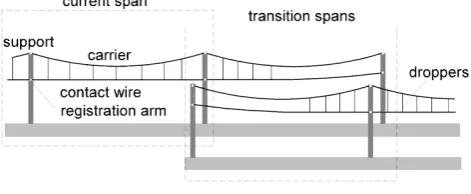
The overhead contact line or catenary is assembled considering a range of spans, normally between 15 and 20, each of them about 60 m. When the catenary is modeled, the different types of elements can be considered: carrier wire, contact wire and droppers. The transition spans of each series are overlapped, and they present a special configuration in the contact wire, in order to make the transition of the pantograph smoother, as we can see in Fig. (1).
As the carrier wire and the contact wire are tightened by pulleys and independent counterbalances, located at the end of each series of spans. The catenary is a continuous system that can be modeled applying the techniques of analysis of the Finite Element Method (FEM), according with [2] and [5].
With respect to the carrier and contact wires, the following Euler-Bernoulli differential equation considering a flexible pre-stressed wire in motion has been considered:
⁄ 0. (3)
Where p is the weight of the wire per unit of length, g is the gravity acceleration, y the vertical position of a generic point of the wire, T the mechanical tension, I the diametric moment of inertia, and E the elastic module of the material.
The wires are modeled as pre-stressed beam elements, with two generalized coordinates by node: the vertical displacement and the turn angle. The droppers behave as elastic bars of final length of assembly, which deform themselves from an initial length. In this case, each node presents only one generalized coordinate corresponding to the vertical displacement.
Notice that the droppers only work in tension, so that, its effect in the dynamic equations, and their inclusion in the stiffness matrix and independent term, will be considered only when the effective final length, measured as the distance between the extreme nodes, will be greater or equal as the initial length. It is supposed that the length and traction tension of the droppers have been calculated in a previous static study.
Figure (1): Catenary with the transition spans overlapped.
The effect of the registration arm has also been considered. This element is an articulated bar whose functionality consists in fixing the contact wire so that it describes a zigzag, to wear out uniformly the pantograph rubbing surface, behaving as a semi-rigid support.
The arm effect on the stiffness matrix and over the independent term can be approximate to a spring of stiffness kb
that exerts a dynamic force over the contact wire, given by the equation:
. (4) Where fA represents the dynamic force exerted by the arm, f0
the static force of assembly, y0 is the assembly static height of
the grip node (this is also a fixed value), yA is the generalized
coordinate that is associated to the grip node of the arm, and kA
is the stiffness of the arm, that is getting with the linearization of the statics equations and it depends on the conditions of assembly.
For the mass matrix of the wires, a diagonal matrix has been supposed. With all these considerations, it is possible to assembly the mass matrix, the stiffness matrix, and the independent term in the catenary.
For the damping matrix of the catenary, we have supposed a Rayleigh type damping, according with [2] and [5], where the damping matrix, is a lineal combination of the mass and stiffness matrices.
. (5)
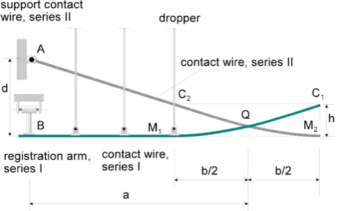
[image:2.595.309.545.121.218.2]Figure (2): Details of the contact wires in a transition span. It is supposed that the trajectory of the pantograph goes from left to right, the span of the series I in Fig. (2), is the output transition span and the span of the series II, is the input transition span, both of them have a symmetric configuration, whose half left part is represented in Fig. (2).
It can be noted that the span of the series I presents a zone of droppers, on the left part. From the last dropper, the contact wire lifts itself until the support on the right side of the span.
The contact wires from both spans intersect in the Q point that is situated in the middle of the span. In order to get a suitable configuration, it would be adequate to specify the droppers position and the height of the support point A of the contact wire, given by the distance d, if E is the elasticity of the catenary in the middle of the span and F is an average estimation of the vertical force of the pantograph that is going to circulate around the line, this force will produce an elevation
h at the wires given by:
. . (6) There is a part of the contact wire that hangs free between the last dropper and the support, and which presents a parabolic configuration, where M1 and M2 are the minimum of the contact
wires of the spans in both series. The elevation h can be used to define a segment of parabola between the points M1 and C1
from the series I or M2 and C2 of the span from the series II, that
in absence of dynamic effects, guarantees the common contact of the pantograph with the two contact wires, for this, the intersect point Q, of the wires situated in the center of the span, has to be in the middle of the points M1 and C1 or M2 and C2.
Let T the mechanical tension of the contact wire, and p the weight of the wire by unit of length, the distance of C1 respect
to the minimum M1 is given by the equations of the statics
wires:
2 ⁄ . (7)
Figure (3): Model of pantograph on two contact wires. If a is the half of the length of the span, the height of the support A of the contact wire in the span of the second series is:
2
⁄ ⁄ 2 . (8) This same height is adopted for the contact wire in the span of the series I assuring, in absence of dynamic effects, the contact of the pantograph with the wires between the points
C2-M2 and C1-M1, however this condition can be changed,
varying the distance from the minimums M1 and M2to the
center of the span Q, obtaining different configurations. In a standard assembly, it is supposed that the center of the span corresponds with the center of the static safe contact zone
C2-M2 and C1-M1, but if we want to get a more precise
configuration we need to introduce dynamics considerations.
V. PANTOGRAPH MODEL
The pantograph is an articulated system that takes the electrical power from the catenary. The pantograph is modeled as a set of masses, springs, and shock absorbers, although the values of these parameters can be obtained by a test in the laboratory, generally, these values are usually specified by the manufacturer. Each mass has a generalized coordinate associated which corresponds to its vertical displacement.
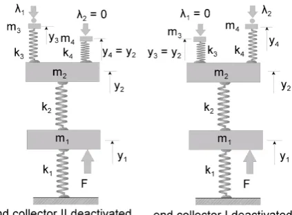
A model of pantograph with two masses is shown in Fig. (3), which is able to interact with the contact wires from the input and output transition spans. To make the differential equation integration easier, two additional elements without any mass have been added over the head mass, called end collectors, which get the force and contact from the wires and are linked to the head mass by a stiff spring, physically the stiffness of this spring represents the real stiffness of the contact wire-platen. λ1
and λ2 represent the constraint forces, or the
[image:3.595.319.542.85.251.2] [image:3.595.47.294.101.254.2]The mass matrix of the pantograph model is a diagonal matrix, with two null elements that correspond to the masses of the end collectors m3 and m4. The mass matrix and stiffness
matrix are as follows:
0 0
0 0
0
0 00 00
0 0 0 0
(9)
0
0
0 0
0
0 .
VI. MODEL OF CONTACT OF THE PANTOGRAPH AND THE WIRE According to previous experiences, to consider a punctual contact between the pantograph and the catenary could represent a problem because it involves to suppose a concentrated force during the motion, and there are integration problems each time that the pantograph goes through a node obtained by the segmentation of the contact wire.
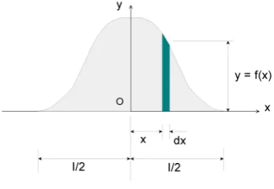
To avoid this problem it would be suitable to suppose a distributed contact, according to a determined distribution function equivalent to say that the contact force is distributed over the rub zone of the pantograph situated at the end collector. By convenience an Oxy axis system, according with Fig. (4), that moves itself with the pantograph is supposed. The x variable represents the position of the different points on the contact wire along the horizontal axis.
Figure (4): Load distribution function.
If l is the length of the rub surface, y3 the generalized
coordinate that corresponds to the vertical position of the end collector, according to the model of Fig. (3), yc(x) is the contact
wire position around the rub surface of the pantograph, and y = f(x), represents the contact distribution function, the following expression is given:
0 . (10) In addition the following expression is fulfilled:
1. (11) These equations allow us to get the end collector position of the pantograph, when the contact wire configuration at instant
tn is known, as a weighed measure of the position of the nodes
of the contact wire that is situated over the rub zone, obtaining the following expression:
. (12) A similar equation is obtained for the position of the other end collector (y4)n. In general a smooth form of the weighed
function y = f(x) is advisable, in order to make the pantograph transition across the nodes easier. Several functions for f(x)
have been tested, and good results have been obtained by using a harmonic function given by:
1⁄ 1 cos 2 ⁄ , ⁄2 ⁄2
0, ⁄ 2 ⁄2. (13) The function yc(x) is the position of the different contact wire
points on the pantograph environment. It can be expressed with the generalized coordinates associated to the nodes from the wire segmentation, according to the FEM. In the same way, the Equation (10) in the tn instant can be expressed in a matrix form,
as follows:
0. (14) The previous expression has to be repeated for all the system constraint conditions, so that the vector øn is converted into the
constraint conditions matrix.
The constraint conditions number depends on the contact wires number over which the pantograph can interact, on the type of pantograph, and on the number of the pantographs along the line. Generally, there are catenaries with direct electrical current with two contact wires, in this case, when the pantograph goes along the transition span, the head mass can interact on four wires.
[image:4.595.62.262.486.624.2]Figure (5): Model of pantograph with different constraint conditions.
VII. CONSTRAINT CONDITIONS MODEL
In order to simplify the constraint condition model presented here, we are going to suppose only a pantograph with one head mass that runs along the catenary which has only one contact wire. A general form of the constraint conditions matrix can be expressed in this case at instant tnas follows:
. (15)
Where the vector ø1n represents the constraint conditions
vector of the end collector I on the contact wire in series I, and the vector ø2n represents the constraint conditions vector of the
end collector II on the contact wire in series II. In the formulation of the equation (15), the following cases have to be considered:
1. The pantograph runs along a current span in series I, it can interact only with only one contact wire. This case is showed in Fig (5).
2. The pantograph runs along a current span in series II, it can interact only with just one contact wire. This case is showed in Fig (5).
3. The pantograph runs along the transition spans; in this case the pantograph can interact with two contact wires. This situation is showed in Fig (3).
In the first case, the vector ø1nis calculated in (10), while the
end collector I position, (y3)n is calculated in (12). On the other
hand, the end collector II can never take contact with the wire in series II, as it is deactivated, and in this case, the constraint conditions vector ø2n, is going to be created imposing the
constraint that the end collector II position, (y4)n and the head
mass, (y2)n, will be coincident, that is:
0. (16) The second case is similar to the previous one, but the end
collector II can contact with the wire and the end collector I will be deactivated. In the third case, the pantograph runs along the transition span and the collectors I and II can contact with the wires in series I and II, and both collectors are activated, the constraint conditions vectors, ø1n and ø2n, are calculated in the
same way, using (10), and the position of the end collectors I and II, (y3)n and (y4)n, are obtained using (12).
Finally, it is important to consider that even though initially the collector is supposed to be interacting with the corresponding contact wire, the contact force can be canceled or have its sign changed. When this happens, the pantograph-cantenary contact does not exist and the constraint conditions have not sense. This circumstance has to be considered when (1) has to be solved. When the collector loses the contact with its respective wire, it is equivalent to make null the stiffness collector.
VIII. NUMERICAL INTEGRATION OF THE DYNAMIC EQUATION The explicit method of the central differences has been used for the integration in (1), for that purpose, the velocity and acceleration vectors of the generalized coordinates have been approximated according to the following expressions:
1 2∆⁄
1 ∆⁄ 2 . (17)
If we replace these equations in (1) the following expression is obtained:
1 ∆⁄ 1 2∆⁄
1 Δ⁄ 2 1 2∆⁄ . (18)
The previous expression allows us to get the generalized coordinates qn+1 in the instant tn+1 but it does not allow us to
know the generalized forces vector λn+1 in that instant. Another
important problem is that to determine qn+1 it is necessary to
solve a lineal system of equations, because the damping matrix
Cn is not diagonal. One of the main advantages of the explicit
methods is that it is possible to obtain the integration variables directly with simple matrix operations, without needing to solve a system with a high number of equations. This could be possible, if we had supposed a diagonal damping matrix for the catenary, or if the damping had not been considered.
Although these options could be legitimate, it has been considered that a Rayleigh type damping is more realistic, according to (5), and to integrate (1) in an efficient way, the velocity vector of generalized coordinates has been modified in half step. It allows us to get the integration variables in a direct form, obtaining the following system of equations:
0
0 0 0 00
⁄
⁄ 0
[image:5.595.60.272.97.253.2]According with [5], this modification introduces a small error that can be ignored if a structural system with a low damping has been considered, as it occurs in our case.
The velocity and acceleration vectors of generalized coordinates have been approached according to the expressions:
⁄ 1 ∆⁄
1 ∆⁄ ⁄ ⁄ (20)
1 ∆⁄ 2 .
These expressions have been replaced in (19), and solving for the generalized coordinates vector qn+1, considering that the
mass matrix is diagonal, the resulting equation is as follows:
1 ∆⁄
1 Δ⁄ Δ / / . (21)
The previous equation allows us to calculate the generalized coordinates vector qn+1. However, there are still some aspects
that are not solved: the generalized force vector λn+1 cannot be
calculated and in addition (21) cannot determine the end collectors positions (y3)n+1, (y4)n+1 because its mass is null, and
this makes the equation useless for its calculation. However, if the end collector is activated, it is possible to calculate its position using (12) in tn+1. If the collector is deactivated, its
position will be the same as the head mass calculated according to (16).
The pantograph-catenary constraint forces are the same as the forces of the springs, because the masses of the end collectors are null:
. (22) Thus, the cycle of integration is completed in tn+1. In order to
initiate the algorithm, the generalized coordinates values and constraint forces at the initial moment have been calculated, solving the following linear system:
0 0 . (23)
In addition to this, with regard to the velocity vector of generalized coordinates in the initial instant, it has been assumed that:
0. (24) The exposed integration procedure, based on the explicit method of the central differences, allows us to obtain the variables carrying out simple operations, without needing to solve systems of equations, treating nonlinearities as a direct form because the different variable terms can be updated: stiffness matrices, damping matrices, constraint conditions and
independent term at the end of each cycle of integration and finally all of them are ready for the following integration cycle.
IX. INTEGRATION ALGORITHM
According to the previous sections, the integration algorithm is organized as follows:
1) Introduction of the assembly data: Carrier and contact wires characteristics: weight, material, section, mechanical tension in the cables, number of contact wires, etc. droppers characteristics: lengths, weight, etc. It is also necessary to consider the data about the pantograph or pantographs: number of pantographs, forces, masses, stiffness, damping, etc.
2) To form the stiffness matrix K0 and the independent term
R0 at the initial instant, according to the supposed model
for wires and pantograph, according to (3), (4), and (9). The Equations (6), (7), and (8) will be used to establish the boundary conditions on the supports of the contact wire, defined by the height of the A point in Fig. (2).
3) To form the constraint conditions matrix at the initial instant, according to (10), (15), and (16). Initially, it has been assumed that the pantograph is located on a current span of the first series of spans.
4) To form the mass matrix M. A diagonal mass matrix will be considered.
5) To form the initial damping matrix of the system C0, using
(5) for the damping matrix of the catenary.
6) To determine the generalized coordinates and initial constraint forces, solving the linear system (23) and making null the velocity vector, according (24).
7) Integration cycle of the differential equations in the time
tn+1, n =0,1,2,..., considering:
7.1) Calculation of the generalized coordinates of the catenary and pantograph qn+1, at the instant tn+1, using
(21).
7.2) Calculation of the end collectors position of the pantograph, (y3)n+1 and (y4)n+1, using (12) or (16),
depending on the pantograph running along a current span or along a transition span.
7.3) Calculation of the constraint pantograph-catenary forces, (λ1)n+1 and (λ2)n+1,using (22).
7.4) To form the constraint conditions matrix øn+1, using
(10), (15), and (16), considering if the pantograph is located on a current span or on a transition span. 7.5) To update the different matrices and independent terms
for the instant tn+1 : Kn+1, Cn+1, and Rn+1, taking into
account the disconnection of droppers and the losses of contact between the pantograph and the catenary. In particular, the effect of the loss of contact will be considered in the following way: according if the pantograph is on a current span or on a transition span, the previously discussed cases will be considered. If the pantograph is on a transition span and the sign of the contact forces (λ1)n+1 and (λ2)n+1,calculated in (22) is
the end collector is working in traction, this is equivalent to make zero the stiffness associated to the end collector. Thus, if k0 represents the real stiffness of
the contact:
0; 0
0; 0. (25) According with this, the stiffness matrix of the system
will be updating for the following step.
7.6) The velocity vector of the generalized coordinates will be calculated too:
⁄ 1 ⁄ ∆ . (26) 7.7) Modification of the subscript of the variables and terms
of the differential equation according to the cycle of integration: the subscript n+1 corresponding to the terms calculated in the present cycle, it is transformed into n, returning to the point 7.1, repeating the process, until the pantograph has completed its trajectory. X. COMPUTATIONAL ASPECTS AND APPLICATIONS The procedures exposed in the previous sections have served as the base for the development of a software application implemented in Visual C language that allows us to simulate the dynamic behavior of the pantograph-catenary system considering two series of spans with transition span and several pantographs.
At the time of developing this software, other important aspects relative to a high performance software have been considered, among others, according with [10]: robustness, portability, and efficiency in terms of reduction of memory requirements (Bytes of memory) and in terms of computational cost of the algorithm (flops).
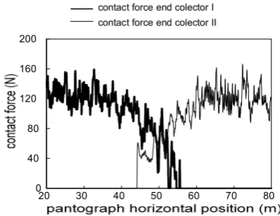
Figure (6): Pantograph-catenary contact force in end collectors. Since the stiffness matrix and the damping matrix present a high sparsity degree, they are stored in one of the storage formats that exist for sparse matrices and that can be found in
scientific literature, according with [11] and [12]. To be precise, two formats have been chosen: The coordinate format (COO) by its simplicity and suitability for this algorithm, and the compressed row format (CSR) that allows us to carry out operations between matrices (matrix vector product, resolution of equation systems, etc) with a simple form. In this way, a reduction of memory requirements have been obtained to store the matrices that appear in the resolution of the dynamic problem, obtaining moreover a considerable reduction in the computation time.
Figure (7): Total pantograph-catenary contact force. On the other hand, the characteristics of robustness, portability and efficiency (in flops), have been obtained thanks to the use of standard linear algebra libraries: BLAS, see [8], and SPARSKIT, see [11].
Thus in the study of a problem with two series of spans of catenary with 1200 m, using elements of 0.2 m, a sparse stiffness matrix for the catenary is obtained K1n, of
48000x48000, nevertheless the no null elements are approximately 4x48000. The memory requirements will be increased when a 3-D model of the catenary would be considered in future works.
Below we present an application of the proposed method, we have considered a simulation with a pantograph of two masses circulating to 120 km/h along two series of three spans, being the central span a current span and both end spans transition spans, the height between wires at the supports is 1.2 m, the material used is copper, the mechanical tension in the carrier and in the contact wire is 10KN with a diameter of 12 mm. The length of the spans is 20 m.
Three droppers in the normal central span of each series have been arranged, separated to at distance of 5 m, and two droppers for the transition spans, being in this case, the distance from the first dropper to the support of 3.83 m and the distance between droppers of 2 m, with the aim of fixing the position of the minimum in the second dropper, getting a contact zone situated in center from the span. The droppers section is 25 mm2.
It has been assumed a model of pantograph similar to Fig. (3), with: m1 =15kg, m2 =7.2 kg, k1 =50N/m, k2 = 4200N/m, k3 = k4
20 30 40 50 60 70 80
0 40 80 120 160 200
contact force end colector I contact force end colector II
20 30 40 50 60 70 80
[image:7.595.323.524.223.373.2] [image:7.595.63.262.517.670.2]= 50KN/m, with a thrust force of F = 120N. The values of the pantograph-catenary contact force in the end collectors on the three central spans are shown in Fig. (6), corresponding to a horizontal displacement of the pantograph between 20 m and 80 m.
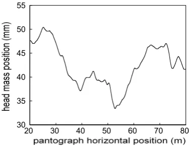
Figure (8): Head mass vertical position.
The pantograph position between 40 m and 60 m corresponds to the transition span. The contact force on the first series is represented by the thick continuous line and the contact force on the second series by the line of fine outlines.
It is possible to observe that the force on the first series is progressively decreasing from 40 m, being completely null for the position of 56 m approximately, whereas the force on the second series appears from 44 m.
The total pantograph-catenary contact force, obtained adding the contact forces of both end collectors, is showed in Fig. (7), it can be noticed that when the pantograph is running on current spans, the contact force varies around 120 N approximately, but when the pantograph is running on the transition span, the total contact force experiments strong variations, especially on the center of the span, (point Q in Fig. (2) ), around this point the contact force oscillates between 80 and 170 N, in this point the contact wires of the transition spans are crossed.
The variation of the vertical position of the head mass is shown in Fig (8). It is possible to observe that when the pantograph runs on current spans, the head mass presents maximum displacements of 50 mm and 47 mm approximately for each span, whereas when the pantograph runs along the transition span, the maximum displacement does not get the 42 mm. The reason for this is because the pantograph must interact in a zone with two contact wires, thus the line presents a greater stiffness. Varying the configuration of the contact wire, it is possible to obtain a smaller variation in the contact force, in order to obtain a smooth transition and a better behavior of the system.
XI. CONCLUSION
In the present work, a procedure for the study and simulation of the dynamic pantograph-catenary system interaction in
railway lines has been developed, considering two series of spans with the both-end spans overlapped. A differential equation system with constraints has been obtained, where the catenary has been modeled using the FEM, whereas the pantograph has been considered as a system of masses, springs, and shock-absorbers. A numerical integration algorithm has been developed based on the explicit method of the central differences, that solves the problem in a simple and direct form, as a differential ordinary equation system, where the pantograph can interact with only one contact wire, when it is running in a current span, or with two contact wires when it runs along the transition span.
The proposed procedure allows us to carry out simulations, in order to obtain optimal assembly conditions in the line. In particular the presented method is adequate to study the most suitable configuration of the contact wire, in order to facilitate the transition of the pantograph from a series of spans to another one, in a smooth way. This procedure can also be implemented in the case of several pantographs running on the line, considering the complete trajectory of the pantographs.
The results of this work have served as the base to implement a software program in Visual C language that allows us to carry out simulations for different types of catenaries and pantographs, getting very low computational times, thanks to a spectacular reduction of the memory requirements. The presented method can be extended for catenaries with two contact wires; this type of catenary is used to impel traction units with direct electrical current, and it is very frequent in conventional lines of several European countries.
It is also possible to extend this procedure to the study of dynamic problems in three dimensions, considering the effect of the wind, curve track etc, being able to obtain very realistic simulations with really reasonable computational times.
REFERENCES
[1] M. Arnold, and B. Simeon, “Pantograph-Catenary Dynamics: A Benchmark Problem and its Numerical Solution”, in Applied Numerical Mathematics, vol. 31, n. 4, pp. 345-362 , 2000.
[2] K. J. Bathe, “Finite Element Procedures”, Prentice Hall, 1996. [3] J. Benet, E. Arias, F. Cuartero, and T. Rojo, “Problemas básicos en el
Cálculo Mecánico de Catenarias Ferroviarias”, in Información Tecnológica, vol. 15, n. 6, pp.79-87, 2004.
[4] A. Collina, and S. Brusi, “Numerical Simulation of Pantograph-Overhead Equipment Interaction”, in Vehicle System Dynamics, vol. 38, n. 4, pp. 261-291, 2002.
[5] D.C. Cook, D.S. Malkus, and M.E. Plesha, “Concepts and Application of Finite Element Analysis”, John Wiley and Sons, 1989.
[6] L. Drugge, T. Larsson, and A. Stensson, “Modelling and Simulation of Catenary-Pantograph Interaction”, in Vehicle System Dynamics, vol. 33 (supplement), pp. 490-501, 1999.
[7] C.N. Jenssen, and H. Trae “Dynamics of an Electrical Overhead Line System and Moving Pantographs”, in XV IAVDS Symposium, 1997. [8] C.L. Lawson, R.J. Hanson, D.R. Kincaid, and F.T. Krogh, “Basic Linear
Algebra Subprograms for FORTRAN Usage”, in ACM Trans.Math. Soft , 1979.
[9] M. Lesser, L. Karlsson, and L. Drugge, “An Interactive Model of a Pantograph-Catenary System”, in Vehicle System Dynamics, vol. 25 (supplement), pp. 397-412, 1996.
[10] B. Nath Datta, “Numerical Linear Algebra and Applications”, Brooks /Cole Publishing Company, 1995.
20 30 40 50 60 70 80
[image:8.595.65.253.162.308.2][11] Y. Saad, “SPARSKIT a Basic Tool Kit for Sparse Matrix Computations”, CSDR, University of Illinois and NASA Ames Research Center, 1994. [12] Y. Saad, “Iterative Methods for Sparse Linear Systems”, PWS Publising
Company, 1996.
[13] M. Schaub, and B. Simeon, “Pantograph-Catenary Dynamics: An Analysis of Models and Simulation Techniques”, in Mathematical and
Computer Modeling of Dynamical Systems, vol. 7, n. 2, pp. 225-238,