Online Full Text



Abstract— Prediction of time series is increasingly becoming popular in many different fields. The forecasting process sometimes is not straight forward due to the presence of a large quantity of data and various parameters. Many techniques can be used to estimate future time series. Nowadays, data-driven approaches can be used for modeling complex phenomena. Artificial intelligence (AI) can be recruited to overcome these complexities. However, sometimes for improving results and exactness of the models, combined models are used, especially for modeling the complex events. In this study, a combined wavelet-ANN is used to predict future rainfall time series a few months in advance. Five different models are defined to assess the skillfulness of each model. The accuracy of the models is evaluated by means of various statistical parameters such as Root Mean Square Error (RMSE), Mean Absolute Error (MAE), and correlation coefficient (R). The results show that the wavelet-ANN model remarkably enhances the capability of the neural network and is a superior method for estimating the complex phenomena and prediction the peak values of time series.

Index Terms— ANN, rainfall, time series, wavelet.

I. INTRODUCTION

N recent years, the wavelet transform has attracted much attention since its advent in signal processing [1]. The wavelet transform was introduced rapidly as an alternative to the Fourier transform. This approach outperforms over traditional spectra analysis methods in non-stationary, multi-scaled and localized phenomena. In other words, providing a time-scale localization of a process is the primary merit of the wavelet transform. Therefore, it is highly suggested for analyzing irregularly distributed events [1].

Hydrological time series such as rainfall time series is more challenging and problematic due to the atmospheric process complications and uncertainty of the rainfall interactions with hydro-meteorological variables. In Australia, rainfall shows a high degree of temporal and

Manuscript received June 24, 2019.

M. Ghamariadyan is with the Swinburne University of Technology, Melbourne, Australia (phone: +61451287833; e-mail: [email protected]).

M. A. Imteaz is with the Swinburne University of Technology, Melbourne, Australia (mimteaz @swin.edu.au).

F. Mekanik is with the Swinburne University of Technology, Melbourne, Australia ([email protected]).

spatial variability which results in some challenges in rainfall prediction [2]. Therefore, finding the reliable and exact models, especially for long-term predictions is of great importance for better management of water resources and disaster controlling, especially in Australia with extreme variability of rainfall.

Nowadays, data-driven approaches can be used for modeling complex phenomena. Artificial Neural Network (ANN) can be recruited to overcome these complexities. However, sometimes for enhancing the accuracy of the models, hybrid models are used especially for modeling the complex phenomena. One of the hybrid models is wavelet-ANN which is becoming a widely used approach in recent years. The use of hybrid approaches has been increased due to their ability to get better results in terms of accuracy. The Wavelet-ANN is one of the methods which is able to improve the results of ANN modeling. Many studies in various fields used application of hybrid wavelet models and it was found that it is possible to take advantage of the neural network and wavelet analysis, simultaneously [3], [4]. Kim and Valdés used wavelet transforms and neural network for forecasting drought in a river basin in Mexico [3]. For modeling sediment discharge, Kisi used wavelet-ANN for assessing the ability of this method for calculating river sediment load [4]. Partal and Cigizoglu applied wavelet-neural network for forecasting daily rainfall time series. They found that a combined model estimates superior results than conventional models [5].

The aim of this study is to develop a reliable model for forecasting rainfall time series using different inputs such as climate indices a few months in advance. The Harrisville in the southeast of Queensland, Australia is selected as a case study. The results are compared to the ANN and observed data obtained from Australian Bureau of Meteorology (BoM) by means of various statistical parameters such as Mean Absolute Error (MAE), Root Mean Square Error (RMSE), and correlation coefficient (R). The different lead times are chosen to show the model ability to forecast the future rainfall time series. In the following section, the wavelet transform is described and, then application of this wavelet transform and artificial neural network is investigated.

Application of Wavelet Transform and Artificial

Neural Networks for Predicting Rainfall Time

Series with Various Variable Inputs

M. Ghamariadyan, M. A. Imteaz, and F. Mekanik.

II. ARTIFICIAL NEURAL NETWORKS

Artificial neural networks are powerful tools that try to imitate human brain properties by learning and training rules [6]. They are widely used black-box models throughout the world. An ANN consists of numerous nodes called neurons that are structured in one or more layers [7]. The most popular ANN is multilayer perceptron (MLP) feed-forward neural network with a back-propagation algorithm. It comprises one or more hidden layers between input and output. The number of hidden neurons can be obtained according to the complexity of the problem through trial and error process. A feed-forward neural network explicitly is described as follows [3]

. 0

1 1

M N

yk f wkjf h w jixi w jo wko

j i

 _{ } 

 

  _   _

 _{   } 

 

(1) where, _{w ji} stands for the hidden layer’s weight which connects the ithneuron in the input layer with the jth neuron in the hidden layer; f ₀ is the activation function for the output layer; _{w jo} is the bias for the jth hidden neuron; _{w kj} represents the output layer’s weight that connects jthneuron with the _kthneuron in the output layer; _{w jo} is the bias for the _kth hidden neuron; _{f h} is activation function and _{y k} is the output of the feed forward neural network. In this study, the number of hidden neurons was chosen based on trial and error using Back-Propagation algorithm. Also, we use the Levenberg– Marquardt (LM) algorithm for training the network. As overtraining may occur during developing any ANN model, some techniques are used to avoid this problem. The early stop technique is used in this study. In this technique, the training process is stopped when validation error begins to increase in spite of diminishing the training set error. In addition, allocating some data for calibrating and testing the model can assure the right performance of the model. In other words, the model is exposed to new data (testing data) which have not been already used by the model.

III. WAVELET TRANSFORM

The advent of wavelet analysis in spectral analysis can be considered as a milestone due to its ability to provide a time-frequency description of a signal in the time domain [8]. The fundamental role of the wavelet is extracting invaluable hidden and nontrivial properties of the time series which cannot be seen in the main signal. The initial theory of the wavelet analysis was derived from the Fourier transform. In Fourier transform, the signal is broken down into some sine waves which are not temporally and spatially localized. A wavelet is a limited duration wave with a mean value of zero. In wavelet analysis, the main time series is decomposed into different lower resolution levels through shifting and scaling factors of a basic wave

called mother wavelet (wavelet function). There are several wavelet functions such as Bior, Morlet, Dmey, Symlet, Db, etc. The Haar wavelet and Daubechies (Db) groups are broadly used in wavelet analysis. Scaling refers to the process of stretching or shrinking the signal in time and shifting is proceeding and delaying a wave along with the signal. Selecting a proper wavelet coefficient is the essential part of the wavelet analysis and it affects the accuracy of the results. A discrete form of wavelet can be described as follows [9]

f a b( , ) a 1/ 2 f t( ) (t b)dt a



 _



 

 (2)

where, ais the scale parameter, b defines the position of the wavelet that demonstrates sliding of the wavelet over

( )

f t ,( )t is the basic wavelet with length (t) which is normally much shorter than the main time seriesThe .f t( ) main signal is decomposed into approximation and detail components and can be described by

f t( )D₁D₂ ... DiAi (3)

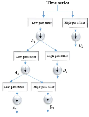
where, Dand Arepresent detail and approximation, respectively.i is the level of decomposition (highest level). Each low-pass filtered component (A) can be decomposed into a high-pass filtered and a low-pass filtered component. For example, A₁ is a low-pass filter which can generate

2

A (a low-pass filtered component) and D2(a high-pass filtered component). Fig. 1 shows the decomposed sub-series of approximation and details for the selected original rainfall time series.

Fig. 1. Process of decomposition the time series.

study, to show the ability of the model to predict the future rainfall time series, three different lead times (1-month, 3-month, and 6-month) are considered.

Fig. 2. Diagram of hybrid wavelet–ANN predicting model.

IV. DATA AND STUDY AREA

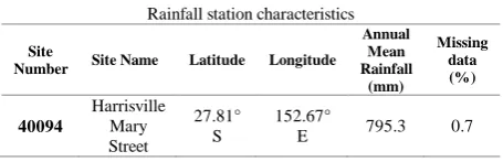
We selected the Harrisville station in the southeast of Queensland as a case study (Fig. 3). This station is chosen because of having a long record of data with few missing values. Moreover, this station is located in the most populated city in Queensland, Australia. Table Ι shows the details of the selected station along with the mean annual rainfall value. The monthly rainfall time series was collected from the Australian Bureau of Meteorology website [10]. The data of 109 years (1908-2016) are used to forecast the rainfall in Queensland. The first 92 years (1908-1999) are assigned to calibration and the remaining 17 years (2000-2016) are used as the out-of-sample set to test the models. Also, in this study, we consider the effect of different climate indices (SOI, IPO, and Nino3.4) on future rainfall. In Australia, climate forecasts are mainly based on large-scale patterns or Southern Oscillation phases [11]. The ENSO is primarily measured by the SOI which is based on the pressure differences between Tahiti and Darwin [12]. The Nino 3.4 anomalies in the equatorial Pacific Ocean monitors the sea surface temperature. The IPO, which is similar to ENSO is defined by changes in the SST in the Pacific Ocean. However, the IPO has an irregular inter-decadal cycle, unlike ENSO. The data related to Nino 3.4 is obtained from the Royal Netherlands Meteorological Institute (KNMI) Climate Explorer [13]. The time series values of SOI were acquired from the Bureau of Meteorology (BOM) and the monthly values of IPO were obtained from Chris Folland, Met Office, Hadley Centre, UK [14].

TABLE Ι Rainfall station characteristics

Site

Number Site Name Latitude Longitude

Annual Mean Rainfall

(mm)

Missing data (%)

40094

Harrisville Mary Street

27.81° S

152.67°

E 795.3 0.7

For assessing the skillfulness of the ANN and wavelet-ANN model, five different models comprised of rainfall and climate indices are defined different combinations of past rainfall time series and climate indices are explored to obtain the best models (Table II). These models are chosen

Fig. 3. Location of the study area and rainfall station.

TABLE II. Model inputs Model Input variable

Ι Rainfall

II IPO

III SOI

IV Nino 3.4

V Rainfall+IPO+SOI+Nino+Max Temp+Min Temp

based on the effect of climate indices on Queensland rainfall and also past research in this region.

To assess the skillfulness of each model, different statistical parameters such as the Root Mean Squared Error (RMSE), and Mean Absolute Error (MAE) are used.

V. RESULT AND DISCUSSION

The results of calibration and testing the models are shown in Table III, IV, and V for one, three, and six months lead times. The capability of the various models of ANN and wavelet-ANN for predicting the rainfall time series are assessed. The first model is a unary model with one input which is defined as a base model for comparing with other models and the fifth model is a comprehensive model which consider the effect of different parameters in forecasting rainfall. Table III shows the skilfulness of the wavelet-ANN versus ANN technique.

TABLE III

Accuracy of the calibration and testing at one month lead time

Model Calibration Testing RMSE MAE R RMSE MAE R

ANN

Ι 59.33 42.21 0.41 51.19 37.72 0.41 II 64.22 47.9 0.22 58.1 45.8 0.2 III 62.84 45.39 0.27 56.38 44.14 0.26 IV 61.98 44.56 0.32 55.3 40.92 0.31 V 57.89 40.55 0.46 49.47 37.6 0.54

HWNN

Ι 4.19 1.46 0.99 3.40 1.82 0.99 II 60.86 47.36 0.2 56.78 44.65 0.35 III 62.69 46.6 0.28 56.71 24.32 0.26 IV 63.37 47.25 0.25 56.27 44.41 0.34 V 4.32 2.84 0.99 5.89 4.51 0.99

TABLE IV

Accuracy of the calibration and testing at three months lead time.

Model Calibration Testing RMSE MAE R RMSE MAE R

ANN

Ι 59.31 42.87 0.42 54.58 38.5 0.49 II 61.05 44.75 0.35 57.37 43.28 0.38 III 63.32 46.25 0.24 59.97 47.3 0.27 IV 60.79 45.98 0.32 58.62 44.69 0.35 V 58.35 41.73 0.44 54.16 38.22 0.47

HWNN

Ι 23.25 17.58 0.93 32.94 18.89 0.85 II 62.24 45.39 0.3 59.76 44.8 0.28 III 63.88 47.31 0.22 43.28 0.54 0.28 IV 62.46 46.27 0.3 46.06 0.5 0.24 V 23.68 18.26 0.93 34.01 20.35 0.84

The skillfulness of the models are shown six months in advance in Table V. It is evident that the models developed by wavelet-ANN technique still give better results compared to the ANN method. For the wavelet-ANN, the best models are still the first and last models. However, the accuracy of the ANN remains at a specific range (RMSE values between 53.91 and 64.49).

TABLE V

Accuracy of the calibration and testing at six months lead time.

Model Calibration Testing RMSE MAE R RMSE MAE R

ANN

Ι 60.41 42.99 0.37 55.74 39.33 0.43 II 62.82 44.68 0.3 64.49 47.4 0.17 III 64 47.52 0.24 61.68 47.12 0.21 IV 61.4 42.9 0.36 61.87 45.21 0.23 V 57.97 40.87 0.46 53.91 37.51 0.51

HWNN

Ι 49.6 35.62 0.65 38.82 25.73 0.78 II 61.98 45.01 0.31 61.28 44.93 0.22 III 64.88 47.98 0.12 61.14 46.43 0.26 IV 63.89 47.44 0.23 57.78 43.97 0.37 V 37.46 27.76 0.81 44.25 29.77 0.73

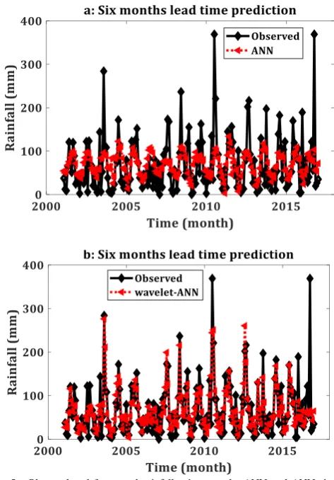
The plot of observed rainfall and forecasted rainfall in different lead times are depicted in Fig. 4 and Fig. 5for the testing period in the wavelet-ANN and ANN modeling based on best input combinations. It can be seen that wavelet-ANN model predicts future rainfall one month in advance with high accuracy (almost same as observed time series). However, the ANN model is not able to produce accurate results. In Fig. 5, the forecasted future rainfall time series are compared with observed time series at six month lead time. It is evident that the wavelet model still

Fig. 4. Observed and forecasted rainfall using wavelet-ANN and ANN one month in advance.

generates better results in contrast to the ANN model. It is noteworthy that the wavelet-ANN captures the extreme values of time series with good accuracy. This would be very invaluable in prediction the possible future flood and drought.

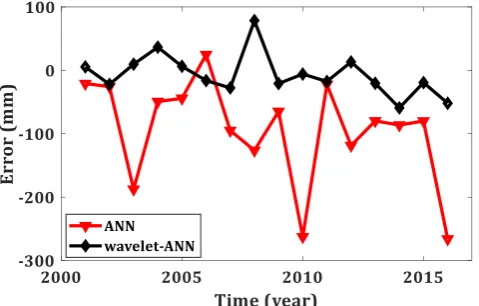
In Fig. 6 the error of peak annual rainfall is shown by the wavelet-ANN and ANN at three months lead time. It is evident that the wavelet-ANN model estimates the annual peak error with the values between -50 mm and +50 mm. However, these values range between +50 mm and -300 mm for the ANN modeling. It means that the ANN model underestimates the peak values of rainfall time series.

Although by increasing the lead times (from three to six months) accuracy of the modeling decreases, the error of annual peak rainfall values in the forecasting of rainfall six months in advance remains relatively at the same range as the three months lead time prediction (Fig. 7).

Fig. 6. Estimation of the error of annual peak at three months lead time.

Fig. 7. Estimation of the error of annual peak at six months lead time.

VI. CONCLUSION

The advent of hybrid techniques such as wavelet-ANN gives a chance to researchers to investigate complex phenomena such as climatological events precisely and also help them to have better insight into them. In this study, we used wavelet-ANN and ANN methods for forecasting future time series of rainfall. The wavelet transform can capture useful hidden information of rainfall and climate drivers which cannot be seen in the main time-series. To the best of our knowledge, as by proceeding in lead times the accuracy

of the prediction will decrease, this technique can improve the skilfulness of the results in spite of increasing the lead times from 3 months to 6 months. The different models were defined to consider the impact of various effective anomalies on rainfall time series. The skillfulness of the model was evaluated by RMSE, MAE, and correlation coefficient.

It was found that the wavelet transform can enhance the results and it can be considered as a superior method for estimating the extreme rainfall in various lead-times. It was also shown that the proposed wavelet-ANN model reproduces better results compared to the ANN model. To the best of our knowledge, the WNN models are reliable in forecasting complex time series with excellent accuracy.

The contribution of this work is developing a novel model for predicting rainfalls one, three, and six months in advance. Also, the novel model and results obtained in this work can be extended to a model in which more than four climate indices can be recruited in modeling the rainfall with remarkable results. The developed models especially performed well in forecasting rainfalls six months in advance with high accuracy. It is to be noted that no such monthly rainfall forecasting model has been yet presented for the Queensland region with such level of accuracy.

REFERENCES

[1] A. Grossman, and J. Morlet, “Decomposition of Hardy functions into square integrable wavelets of constant shape,” SIAM journal on

mathematical analysis, vol. 15, no. 4, pp. 723–736, 1984.

[2] B. Sivakumar, F. M. Woldemeskel, and C. E. Puente, “Nonlinear analysis of rainfall variability in Australia,” Stochastic Environmental Research and Risk Assessment, vol. 28, no. 1, pp. 17-27, 2014. [3] T. W. Kim and J. B. Valdés, “Nonlinear model for drought forecasting

based on a conjunction of wavelet transforms and neural networks,” Journal of Hydrologic Engineering. vol. 8, no. 6, pp 319–328, 2003. [4] Kisi O, “Daily suspended sediment estimation using neuro-wavelet

models,” International Journal of Earth Sciences, vol. 99, no. 6, pp. 1471–1482, 2010.

[5] T. Partal and H. K. Cigizoglu, “Prediction of daily precipitation using wavelet-neural networks,” Hydrological sciences journal. Vol. 54, no. 2, pp. 234–246, 2009.

[6] C. T. Hsieh, “Some potential applications of artificial neural systems in. Journal of Systems Management,” vol. 44, no. 4, pp. 12, 1993. [7] S. Haykin, “Neural networks: A comprehensive foundation,”

Mac-Millan, New York 696, 1994.

[8] I. Daubechies, “The wavelet transform, time-frequency localization and signal analysis”. IEEE transactions on information theory, vol. 35, no. 5, pp. 961–1005, 1990.

[9] S. G. Mallat, “A Wavelet Tour of Signal Processing,” second edition, Academic Press, San Diego, 1998.

[10] Australia’s official weather forecasts and weather radar-Bureau of Meteorology. Available: http://www.bom.gov.au

[11] B. F. Murphy and J. Ribbe, “Variability of southeastern Queensland rainfall and climate indices,” International Journal of Climatology: A Journal of the Royal Meteorological Society, vol. 24, no. 6, pp.703-721, 2004.

[12] J. S. Risbey, M. J. Pook, P. C. McIntosh, M. C. Wheeler and H. H. Hendon, “On the remote drivers of rainfall variability in Australia,” Monthly Weather Review, vol. 137, no. 10, pp. 3233-3253, 2009. [13] Royal Netherlands Meteorological Institute (KNMI) Climate Explorer.

Available: http://www.climexp.knmi.nl