Solving Second Order Linear Dirichlet and Neumann Boundary Value Problems by Block Method

Solving Second Order Linear Dirichlet and Neumann

Boundary Value Problems by Block Method

Zanariah Abdul Majid, Mohd Mughti Hasni and Norazak Senu

Abstract—In this paper, the direct three-point block one-step methods are considered for solving linear boundary value problems (BVPs) with two different types of boundary conditions which is the Dirichlet and Neumann boundary conditions. This method will solve the second order linear BVPs directly without reducing it to the system of first order equations. The direct solution of these two types of BVPs will be calculated at three points simultaneously using constant step size. This method will be used together with the linear shooting technique to construct the numerical solution. The implementation is based on the predictor and corrector formulas in the PE(CE)r mode. Numerical results are given to show the performance of this method compared to the existing methods.

Index Terms—dirichlet boundary value problems, neumann boundary value problems, block method

I. INTRODUCTION

ANY problems in science and technology are

formulated in boundary value problems as in diffusion, heat transfer, deflection in cables and the modeling of chemical reaction. There are several types of boundary value problems (BVPs) and some of them depend on the boundary condition itself. In this paper, we consider the second order linear two-point BVPs which as follows:

 

'

 

 

,

''

x r y x q y x p

y    q

 

x 0,

 

a

,

b

(1)

with the Dirichlet boundary conditions:

 

a 



y and y(b) (2)

and with the Neumann boundary conditions:

 

 a

y and y

 

b . (3)

Manuscript received March 23 2013; revised April 10, 2013. This work was supported in part by the Graduate Research Fellowship (GRF) from University Putra Malaysia and MyMaster from the Ministry of Higher Education.

Zanariah Abdul Majid is a lecturer at the Mathematics Department, Faculty of Science and also as associate researcher at the Institute for Mathematical Research, Universiti Putra Malaysia, 43400 Serdang Selangor DE, Malaysia (e-mail: [email protected]).

Mohd Mughti Hasni is a Master student at the Institute for Mathematical Research, Universiti Putra Malaysia, 43400 Serdang Selangor DE, Malaysia (e-mail: [email protected]).

Norazak Senu is a lecturer at the Mathematics Department, Faculty of Science, Universiti Putra Malaysia, 43400 Serdang Selangor DE, Malaysia. (e-mail: [email protected]).

Theorem:

Suppose the function f in the BVPs in (1) is continuous on the set





_



 _{    }  _x,y,y' _{a x b, y , y}'

D ,

and the partial derivatives f_yand '

y

f are also continuous on

D. If

(i) f_y

 

x,y,y' 0for all



x,y,y'



D, and (ii) A constant M exists, with



, , '



,

' x y y M

f_y  for all



x,y,y'



D

Then, the BVPs has a unique solution.

Corollary:

In linear BVPs in (1) satisfies

(i) p(x),q(x), and r(x) are continuous on

 

a

,

b

, (ii) q(x) > 0 on

 

a

,

b

,

then, the problem has unique solution.

In literature, there are several researcher that has been conducted the research for solving the BVPs such as Wang et al. [14], Emad et al. [9] and Bongsoo [13].

Adomian Decomposition Method (ADM) has been widely used by many researchers for solving differential and integral problems. However, this method has dealt with some difficulties for solving the problem involving with the boundary conditions. Thus, Bongsoo [13] in 2008 have

proposed a method called the Extended Adomian

Decomposition Method (EADM) for solving the two-point linear and nonlinear second order boundary value problems. Bongsoo [13] managed to overcome the problems inhibit in the ADM by creating a new canonical form containing all boundary conditions make it suitable for solving the BVPs. Finite Difference (FDM), Finite Element (FEM) and Finite Volume (FVM) methods have been proposed by Fang et al.

[2] in 2002 to solve the two-point BVPs. The comparison in terms of the accuracy has been made between these three methods and the results shown that they are comparable to each other with no remarkable differences. Later in 2006, Caglar et al. [1] have proposed a new method called the B-spline Interpolation (CBIM) to compare the accuracy of the results obtained with the methods proposed by Fang et al. [2] in 2002. Clearly, the CBIM managed to give better results. A few years later, Hamid et al. [3] have proposed a new method called the Extended Cubic B-Spline method (ECBIM) for solving the linear two-point BVPs by applying the same procedure in CBIM in [1] but using the extended version cubic

M

IAENG International Journal of Applied Mathematics, 43:2, IJAM_43_2_04

B-spline. Hamid et al. [3] have compared the results obtained by ECBIM with the CBIM in [1], FDM in [2], FEM in [2] and FVM in [2]. The results have shown that this method which is the ECBIM was better in terms of their accuracy.

Many works has been done to solve the BVPs with the Dirichlet boundary condition but there is not much attention pay to the BVPs with the Neumann boundary condition. However, there are several researcher that have shown their interest for solving the BVPs with the Neumann boundary conditions such as Li-Bin et al. [11], Ramadan et al. [10], Emad et al. [9] and Siraj-ul-Islam et al. [12].

Ramadan et al. [10] in 2007, have proposed the polynomial and nonpolynomial spline approaches to the numerical solution of second order BVPs subjected to Neumann boundary conditions. The numerical results have shown that the accuracy of the nonpolynomial spline method was better than the two polynomial spline methods which are the quadratic and cubic splines. Recently in 2011, Li-Bin et al.

[11] managed to come out with a new numerical based on the interpolation by quartic spline functions to solve the second order BVPs with Neumann conditions. Li-Bin et al. [11] have compared their numerical result with Ramadan et al. [10]. The results have shown that the method proposed by Li-Bin et al.

[11] was better.

Several researchers such as Fatunla [4], Majid et al. [5], Rosser [7] and Shampine et al. [8] have proposed a block method which computes simultaneously the solution values at different points along the interval. One-step block method being referred as one previous point to obtain the solution. Recently in 2011, Mukhtar et al. [15] have derived the three-point block one-step method in their paper for solving general second order ordinary differential equations (ODEs) directly without reducing it into the system of first order equations. The results showed that it is better in terms of the accuracy and the computed times. Thus, we are motivated to implement this method for solving the two types of linear BVPs subjected to the Dirichlet and Neumann boundary conditions respectively.

In this research, we will extend the idea in [15] for solving (1) with both condition (2) and (3) respectively without reducing it into the system of first-order ODEs by using the direct three-point block one-step methods with the linear shooting techniques for solving second order linear Dirichlet and Neumann BVPs.

II. FORMULATION

The formulation of the direct three-point block one-step method for solving second order linear BVPs will be based in Mukhtar et al. [15]. This method will compute three approximation values which is y_n1at x_n1 ,y_n2 at x_n2and

3



n

y at x_n3simultaneously.

In Fig. 1, the interval of

 

a

,

b

need to be divided into a series of block with each block containing three points with the step size 3h. Then, the solution obtained in the last point within the k th block will be restored as the initial value for the next block. The same procedure will be repeated to compute the solutions until the end of the interval. This method possesses the desirable feature of one-step method in which

being referred to only one previous point to obtain the solutions.

n

x xn1 xn2 xn3 xn4 xn5 xn6

Fig. 1. Three-Point Block One-Step Method

By letting the second order differential equation as follows:



x y y



f

y , ,  . (4)

The approximating values for y_n1,y_n2 and y_n3 was obtained by integrating once and twice over (4) with respect to x. The evaluation of the first point will be approximated by integrating (4) once and twice at both sides over the interval



xn,xn1



as follows:

 







 



 1 1 ' '' , , , n x n x n x n x dx y y x f dx x y (5)

 













   x n x x n x n x n x n x n x dxdx y y x f dxdx x

y , , ' .

1 '' 1 (6) Therefore,



_





 











1 ' ' 1 ' _{, , ,} n x n x n

n y x f x y y dx x y (7)



_

  

 

 









_ 







1 ' 1 '

1 , ,

n x n x n n n

n y x hy x x x f x y y dx x

y (8)

Thus, Lagrange interpolating polynomial will

replace the f



x,y,y'



in (7) and (8). The

interpolation points involved are



xn,fn



,



xn1,fn1



,



xn2,fn2



and



x

n3

,

f

n3



within the block. By doing that, we will obtain the Lagrange interpolating polynomial which as follows:

































































₃.

2 3 1 3 3 2 1 2 3 2 1 2 2 3 1 1 3 1 2 1 1 3 2 3 2 1 3 2 1                                                           n n n n n n n n n n n n n n n n n n n n n n n n n n n n n n n n n n n n n n n n f x x x x x x x x x x x x f x x x x x x x x x x x x f x x x x x x x x x x x x f x x x x x x x x x x x x P (9)

h h h

3h

IAENG International Journal of Applied Mathematics, 43:2, IJAM_43_2_04

Now, by takingxxn3sh,

dx



hds

and replace it into (7)

and (8). Then, taking -3 to -2 as the limit of integration in (7) and (8) and the corrector formulae for the first point will be obtained as follows:



1 2 3



1 9 19 5

24   

      

 _{n n n n n}

n f f f f

h y y

   

 

 

 

  

 

 

3 2

1 2

1

8 39

114 97

360 n n

n n

n n n

f f

f f h y h y y

(10)

Next, the same process will be repeated similar as the corrector formulae for the first point but the integration point is within the interval



xn_1,xn_2



and the limit of integration is from -2 to -1 in order for us to obtain the corrector formula for the second point. Thus, the corrector formulae which is the approximate value of y_n2 andy_n2obtained would be as

follows:



1 2 3



1

2 13 13

24   



       

 _{n n n n n}

n f f f f

h y y

   

 

 

     

 

 

 

3 2

1 2

1 1 2

7 66

129 8

360 n n

n n

n n n

f f

f f h y h y y

(11)

The corrector formulae for the third point would be obtained by using the same process to obtain the corrector formulae for the first and second point except their integration points. The integration points would be within the interval



xn₂,xn₃



. By

taking the limit of integration from -1 to 0, the corrector formulae obtained would be as follows:



1 2 3



2

3 5 19 9

24   



      

 _{n n n n n}

n f f f f

h y y

   

 

  

   

 

 

 

3 2

1 2

2 2 3

38 171

36 7

360 _{n n}

n n n

n n

f f

f f h y h y y

(12)

III. IMPLEMENTATION

The evaluation of the approximation pointsy_n1, y_n2 and

3



n

y will be based on the PE(CE)rmode where P, E and C

stands for predictor, evaluation and corrector respectively. For each step, r functions evaluation will be used until the convergence is satisfied. The Modified Euler method will be used as the predictor in this algorithm. This method will act as the initial starting point before the corrector formulae take place to compute the approximation values fory_n1, y_n2

andy_n3. The same process will be used for each block along

the interval until the end of it.

There are two types of BVPs that we need to solve in this research which is the BVPs with the Dirichlet boundary

conditions and BVPs with the Neumann boundary conditions. The implementation for solving these two types of BVPs was basically the same but there are slightly differences which can be seen as shown below:

To solve the BVPs, the linear shooting technique will be used together with the direct three-point block one-step method. The BVPs (1) with the Dirichlet boundary conditions will be replaced into two initial value problems (IVP) which as follows:

 

₁'

 

₁

 

,

''

1 p x y qx y r x

y    y1

 

a ,

 

0

' 1 a 

y ,

 

 

2 '

2 ''

2 px y qx y

y   y2

 

a 0,

 

1

' 2 a 

y

.

(13)

Then, by solving the two IVP which is the nonhomogeneous and homogeneous equation in (13), the linear shooting methodwas obtained which as follows:

 

x y

 

x wy

 

x

y  1  2

,

where .

) (

) (

2 1 b y

b y

w  (14)

The same procedure will be used for solving the BVPs with

the Neumann boundary conditions with a slightly

modifications in terms of the initial conditions and the linear shooting method. First, the BVPs (1) with the Neumann boundary conditions will be replaced into two IVP with their initial conditions which as follows:

 

₁'

 

₁

 

,

''

1 p x y qx y r x

y    y1

 

a 0, y

 

a 

'

1 ,

 

'2

 

2 ''

2 px y q xy

y   y2

 

a 0,

 

1

' 2 a 

y

.

(15)

Then, by performing the linear combination between this two IVP in (15), the linear shooting method will be obtained which as follows:

 

x y

 

x wy

 

x

y  1  2 , where

 

 

b y

b y w

' 2

' 1







. (16)

This method will be implemented with the constant step size

h. The convergence test will be used during the calculation of the approximated solution in the corrector formulae to obtain better accuracy.

The convergence test:

TOL y

y3,r1 3,r 0.1 (17)

where r is the number of iterations and TOL is the tolerance. All problems were tested using the absolute error test. The iterations in the corrector formulae will be repeated until the convergence test was satisfied.

IV. NUMERICAL RESULTS

In this section, six numerical examples are presented. From the six numerical examples that has been tested, there are three

IAENG International Journal of Applied Mathematics, 43:2, IJAM_43_2_04

of them come from the BVPs with the Dirichlet boundary condition and another three from the BVPs with the Neumann boundary conditions. The problems will be tested using direct three-point block one-step method (3BVP).

A. Dirichlet Boundary Conditions

Problem 1

 

( ) cos( ),

'' _{x y x x}

y  

 

0

,

1

 

0 0,

y y

 

1 1,

Exact Solution

 

. 2

) cos( )

1 sinh( 4

2 ) 1 cos( ) 1 sinh( 3 ) 1 cosh( 3

) 1 sinh( 4

2 ) 1 cos( ) 1 sinh( 3 ) 1 cosh( 3

x e

e x

y

x x

   



  

 



Source: Bongsoo [13]

Problem 2

 

'( ) exp( 1) 1,

'' _{   }

x x

y x

y

 

0

,

1

 

0 0,

y y

 

1 1,

Exact Solution

 

x x(1exp(x1)).

y

Source: Hamid et al. [3]

NOTATIONS

MAXE : Maximum Error of the Computed Solution.

ECBIM(N) : Extended Cubic B-Spline Method

Minimizing Using Newton’s Method in Hamid et al. [3].

ECBIM(B) : Extended Cubic B-Spline Method

Minimizing Using Built-In Function in Hamid et al. [3].

EAD : Extended Adomian Decomposition Method

in Bongsoo [13].

3BVP : Implementation of the Direct Three-Point

Block One-Step Method For Solving The Linear Dirichlet and Neumann BVPs.

: Maximum Error of the Computed Solution.

COLHW : Collocation method with the Haar Wavelets in Siraj et al. [12].

SPLINE : Polynomial spline method in Li-Bin et al.

[11].

h : Step size.

TS : Total steps.

TABLEI

NUMERICAL RESULTS FOR SOLVING PROBLEM 1 WHEN h0.125

x MAXE

EAD [13]

TS EAD [13]

MAXE 3BVP

TS 3BVP

8

1 _4.37107

8

7 10 14 .

1  

3

8

2 7

10 07 .

8   2.22107

8

3 _1.05106 *_3.20107

8

4 *_1.14106 _3.12107

8

5 _1.05106 _2.90107

8

6 7

10 07 .

8   2.56107

8

7 _4.37107 _1.30107

TABLEII

NUMERICAL RESULTS FOR SOLVING PROBLEM 2 WHEN h0.1

Existing Method

h = 0.1

MAXE TS x 3BVP

1 . 0 

h

TS 3BVP

ECBIM(N) [3]

ECBIM(B) [3]

6

10 91 .

7  

6

10 73 .

5  

10

0.1 _1.13107

4

0.2 7

10 19 .

2  

0.3 _3.29107

0.4 _3.74107

0.5 _4.17107

0.6 *_4.68107

0.7 7

10 28 .

4  

0.8 7

10 62 .

3  

0.9 _2.62107

TABLEIII

NUMERICAL RESULTS FOR SOLVING PROBLEM 2 WHEN h0.01

Existing Method

h = 0.01

MAXE TS

EAD [13]

x 3BVP

h = 0.01

TS 3BVP

EAD [13] 1.051010 100

0.1 _1.181011

34 0.2 _2.151011

0.3 _2.931011

0.4 _3.491011

0.5 _3.841011

0.6 *_3.961011

0.7 _3.761011

0.8 _3.161011

0.9 _2.001011

In Table I, the comparison has been made between two types of methods which is EAD and 3BVP. The numerical results have been listed and the maximum error for both

IAENG International Journal of Applied Mathematics, 43:2, IJAM_43_2_04

methods has been noted by the asterisk sign. It can be seen

that the maximum error for 3BVP was 3.20107and it was

better than the EAD which is only 1.14106 . Moreover, the total steps for 3BVP was lesser compared to the EAD.

Table II and Table III show the numerical results for problem 2 based on the step size h = 0.1 and h = 0.01 respectively. In table II, the comparison has been made between the ECBIM(N) and ECBIM(B) and the results obtained show that the maximum error for 3BVP was better with lesser total steps. The same thing goes in table III when the step size was 0.01. In this table, 3BVP gave better results compared to the EAD with a lesser total steps.

B. Neumann Boundary Conditions

Problem 3

 



2 4 2



,

''

y x x

y  



 

0

,

1

 

0 0,

' _

y '

 

1 2 ,

e y 

Exact Solution

 

x e x2.

y  

Source: Siraj et al. [12]

Problem 4



3



sin

 

4 cos

 

,

)

( 2 3

''

x x x x x x xy x

y      

 

0

,

1

 

0 1,

' _

y y'

 

1 2sin

 

1,

Exact Solution

 

x

 

x2 1sin

 

x.

y  

Source: Liu et al. [11]

TABLEIV

NUMERICAL RESULTS FOR PROBLEM 3

j h MAXE

COLHW

TS COLHW

MAXE 3BVP

TS 3BVP 3

16

1 _2.90104 16 _6.52107 6 4

32

1 _7.48105 32 _7.12109 11 5

64

1 _1.89105 64 _1.69109 11 6

128

1 _4.76106 128 _5.561011 43 7

256

1 _1.19106 256 _5.441012 86 8

512

1 _2.99107 512 _2.881013 171

From Table IV, the local error was computed at their jth

collocation point x_j where

j



1

,

2

,...,

N

where N is the last number on the interval. The comparison has been made between the two methods which is COLHW and 3BVP.

It’s clear to see that for each different step size, the 3BVP could provide a better result in terms of accuracy at their

j

th

point respectively. For the step size

16 1



h , the local error

was taken at the point number 3 thus giving us the local error for both methods which is the COLHW and 3BVP was

4

10 90 .

2   and _6.52107_{respectively. Furthermore, the total}

steps taken by the 3BVP also were nearly half compared to the COLHW.

From this result, it has been shown that the 3BVP could provide a better result for each different step size with lesser total steps.

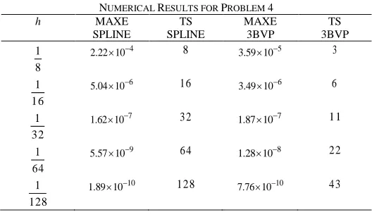
TABLEV

NUMERICAL RESULTS FOR PROBLEM 4

h MAXE

SPLINE

TS SPLINE

MAXE 3BVP

TS 3BVP

8

1 _2.22104 _{8 3.5910}5 ₃

16

1 6

10 04 .

5   16 3.49106 6

32

1 7

10 62 .

1   32 1.87107 11

64

1 _5.57109 _{64 1.2810}8 ₂₂

128

1 _1.891010 _{128 7.7610}10 ₄₃

In Table V, the comparison has been made for each different step size tested at problem 5. The maximum error for both methods which is SPLINE and 3BVP were comparable to each other. In addition to that, the total steps for the 3BVP were lesser as compared to the total steps taken for the SPLINE.

V. CONCLUSIONS

In this research, we have implemented the direct three-point block one-step method together with the linear shooting technique with constant step size which is efficient and suitable for solving the linear Dirichlet and Neumann BVPs directly.

ACKNOWLEDGMENT

The author gratefully acknowledged the financial support of Fundamental Research Grant Scheme (FRGS) and MyBrain scholarship from the Ministry of Higher Education Malaysia.

REFERENCES

[1] H. Caglar, N. Caglar and K. Elfaituri, “B-spline interpolation compared with finite difference, finite element and finite volume methods which applied to two-point boundary value problems”.

Applied Mathematics and Computation, 175, 72-79 (2006). [2] Q. Fang, T. Tsuchiya and T. Yamamoto, “Finite difference, finite

element and finite volume methods applied to two-point boundary value problems”.Journal of Computational and Applied Mathematics,139(1), 9-19 (2002)

IAENG International Journal of Applied Mathematics, 43:2, IJAM_43_2_04

[image:5.612.307.571.221.375.2]

[3] N. N. A. Hamid, A. A. Majid, and A. I. M. Ismail, “Extended cubic B-spline Method for Linear Two-Point Boundary Value Problems”,

Sains Malaysiana, 40(11), 1285-1290 (2011)

[4] S. O. Fatunla, “Block methods for second order ODEs”.

International Journal of Computer Mathematics, vol. 41, pp. 55-63 (1991)

[5]. Z. A. Majid, N.Z. Mokhtar and M. Suleiman, “Direct Two-Point Block One-Step Method for Solving General Second-Order Ordinary Differential Equations”, Mathematical Problems in Engineering, vol. 2012, Article ID 184253, 16 pages, 2012. doi:10.1155/2012/184253 (2011)

[6] Z. A. Majid, P.S. Phang and M. Suleiman, “Application of block method for solving nonlinear two point boundary value problem”,

Advance Science Letter, vol. 13, pp. 754-757 (2012)

[7] J. B Rosser, “A Runge-Kutta for all seasons”, SIAM Review, vol. 9, pp. 417-452 (1967)

[8] L. F. Shampine and H. A. Watts, “Block implicit one-step methods”,

Mathematics of Computation, vol. 23, pp. 731-740 (1969)

[9] H. A. Emad, E. Abdelhalim and R. Randolph, “Advances in the Adomian decomposition method for solving two-point nonlinear boundary value problems with Neumann boundary conditions”,

Computer and Mathematics with Applications, 63(2012) 1056-1065 (2012)

[10] M. A. Ramadan, I. F. Lashien and W. K. Zahra, “Polynomial and nonpolynomial spline approaches to the numerical solution of second order boundary value problems”, Applied Mathematics and Computation, 184 (2007) 476-484

[11] L. Li-Bin, L. Huan-Wen and C. Yanping, “Polynomial spline approach for solving second-order boundary-value problems with Neumann conditions”, Applied Mathematics and Computation, 217 (2011) 6872-6882

[12] U. I. Siraj, A. Imran and S. Bozidar, “The numerical solution of second-order boundary-value problems by collocation method with the Haar wavelets”, Mathematical and Computer Modelling 52 (2010) 1577-1590

[13] J. Bongsoo, “Two-point boundary value problems by the extended Adomian decomposition method”, Journal of Computational and Applied Mathematics, 219(1), pp. 253-262 (2008)

[14] Y.G. Wang, H.F. Song and D. Li, “Solving two-point boundary value problems using combined homotophy perturbation method and Green’s function method”, Applied Mathematics and Computation,

212(2), pp. 366-376 (2009)

[15] N.Z. Mukhtar, Z.A.Majid and F.Ismail, “Solutions of general second order ODEs using direct block method of runge-kutta type”, 7(2).pp. 145-154. ISSN 1823-5670 (2011)

IAENG International Journal of Applied Mathematics, 43:2, IJAM_43_2_04