Abstract—This paper presents a study concerning the structural and mechanical design in Solid Works completed with a kinematic numerical description for a new leg exo-skeleton proposed for human motion assistance and rehabilitation. The exoskeleton proposed new design is based on a seven links mechanism, designed to fulfil human locomotion tasks. A kinematic model of the proposed mechanism is presented and obtained results with a computational algorithm developed in ADAMS, are presented with plots. A 3D model is designed for simulation purposes in ADAMS multi body dynamics software and future manufacturing. The obtained simulation results are useful to appreciate the exoskeleton performance for human rehabilitation purposes.
Index Terms—exoskeleton, kinematics, design, simulation.
I. INTRODUCTION
ODAY, the subject of exoskeleton design for human motion assistance and rehabilitation is present in a large number of studies. In the domain of medical recovery, the locomotors recovery is practiced for patients who have suffered strokes or spinal cord injuries, to be able to practice walking again. The first research study presented in this area, of powered exoskeleton systems, dates from 1960, and this initiative belongs to two separate groups of researchers, one from the US and one from the former Yugoslavia. The first group of researchers is aimed at developing a new technology to help and improve the abilities of the human carrier body, often for military purposes, meanwhile the second group of researchers attempted to produce a technology for motion assistance of people with locomotion disabilities. Currently, are published a large number of papers and research articles for study the human motion assistance and rehabilitation. For disabled people’s motion assistance, exoskeleton systems, active foot orthosis are developed by representative research centers, in order to assist the rehabilitation therapy. Relevant existing systems are discussed in review articles, [1, 2, 3, 4, 5], published by Chen, (2016), Anama et. al (2012), Diaz (2011), Yan (2015). The collective of the authors of present research study presented several design solutions and developed products in papers published by: Dumitru (2015), Geonea (2015-2018), [6-11]. The main purpose of these
Manuscript received March 02, 2019; revised March 09, 2019. I. Geonea is with Faculty of Mechanics, University of Craiova. Calea Bucuresti Street no. 113. Romania (e-mail: [email protected]).
P. Rinderu is with Faculty of Mechanics, University of Craiova. Calea Bucuresti Street no. 113. Romania (e-mail: [email protected]).
achievements is to develop a single degree of freedom human like leg mechanism. In addition, an important task of these systems is represented by the low cost and easy operation feature and facile implementation in practice. In this paper a new exoskeleton leg solution is proposed. The novel exoskeleton is designed based on low cost and easy operation implementation in practical activities. The design solution is studied based on the results of numerical simulation from ADAMS dynamic simulation software.
II. HUMAN GAIT EXPERIMENTAL STUDY
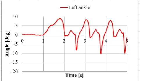
[image:1.595.306.549.404.542.2]For human motion biomechanics, exists on the market, a large number of equipment’s and software to study human gait motion parameters. In this study, the equipment consists in six goniometers sensors attached to human leg joints. A healthy male of 1.68 m height, 68 kg, age 35, represents the subject of this study, by using goniometers sensors on each joint.
Fig. 1. Right ankle joint angle variation in time.
Fig. 2. Left ankle joint angle variation in time.
Design and Kinematics of a New Leg
Exoskeleton for Human Motion Assistance
Ionut Geonea and Paul Rinderu, Member, IAENG
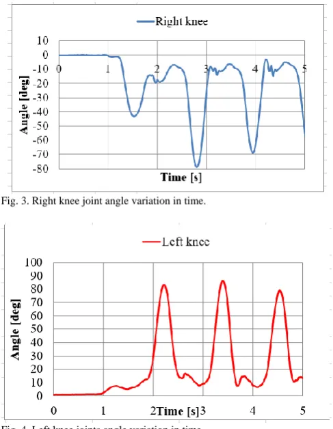
[image:1.595.306.549.578.719.2]Fig. 3. Right knee joint angle variation in time.
Fig. 4. Left knee joints angle variation in time.
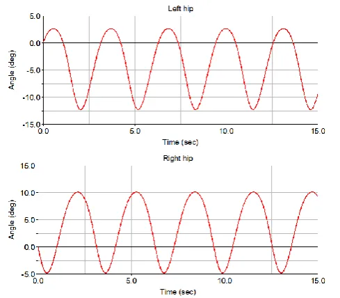
[image:2.595.216.528.387.759.2]With the aid of Biometrics software and goniometer sensors, the angular variations of each joint were acquired and plotted, in Figs. 1-6. The obtained results are compared with others results obtained for human gait and presented in the literature [7]. The conclusion is that the obtained results are usual for normal gait. The knee angle amplitude reaches 60°, as is plotted in Figs. 3-4, and the hip joint angle amplitude reaches 35-40°, as is plotted in Fig. 5-6.
[image:2.595.46.289.474.781.2]Fig. 5. Left hip joint angle variation in time.
Fig. 6. Left hip joint angle variation in time.
III. LEG EXOSKELETON MECHANISM DESIGN
The kinematic scheme of the mechanism for the assistant's exoskeleton legs is shown in Fig. 7. The proposed leg mechanism is composed by a pantograph mechanism completed with a Chebyshev mechanism.
1 2
3 4
5
6 7
A B
C E
D,D*
I H
G F
M
Fig. 7. A kinematic scheme of the proposed leg.
[image:2.595.52.286.479.611.2]The links are noted with digits from (1) to (7) and the joints with letters. The motor link of the mechanism is denoted with (1). The link (7) represents the femur, the tibia link is (6), the joint F represents the hip joint, and the knee joint is denoted with H. The size of the links (6) and (7) can be adjusted so that the shape of the point M trajectory to be an ovoid one, as to human gait.
This leg mechanism can assure the mobility of knee and hip joints. The ankle joint it is not considered because the design solution wants to be a low cost one.
IV. A KINEMATIC ANALYSIS
A theoretical analysis of the leg exoskeleton kinematics was performed in order to evaluate and simulate performances and operation. The point M position, reported to the XY reference system, Fig. 7, is evaluated as a function of input angle φ1 and dimensional parameters of the linkage. Geometrical parameters are:
-fixed joints coordinates: A, F, E. xF=yF=0; xA=182.27 mm;
yA=-247,36 mm; xE=108,97 mm, yE=-217,40 mm.
-links length: lAB=12,5 mm; lBD=82 mm; lBC=45 mm; lEC=69 mm; lDG=250 mm; lID=312 mm; lHF=450 mm; lHM=440 mm. Are known the geometrical dimensions: lAB=12,5 mm;
xA=182.27 mm; yA=-247,36 mm. It is considered an angular velocity of link (1) equal to 2 rad/sec. The coordinates of the joint B are computed with Eq. (1).
1 1
d
t
dt
;
1
2
rad s
/
.
1 1
cos
sin
B A AB
B A AB
x
x
l
y
y
l
(1)Are known the joints coordinates:
x
B,
y
B ; xE=108,97 mm, yE=-217,40 mm.Is writhed the equation (2), to compute the joint C coordinates:
3 2
3 2
cos
cos
sin
sin
C B BC E EC
C B BC E EC
x
x
l
x
l
y
y
l
y
l
(2)In order to compute the angle
2, are grouped the terms that contain the other unknown
3. After square and sum Eq. (3) is obtained a trigonometric Eq. as (4).
3 2 3 2cos
cos
sin
sin
BC E B EC
BC E B EC
l
x
x
l
l
y
y
l
(3)We use the notations:
x
E
x
B
a
1;
y
E
y
B
a
2.
2 2 2 2
1 2
2
1cos
22
2sin
2BC EC EC EC
l
a
a
a l
a l
l
(4) The Eq. (4) can be writhed as (5):
2 2 2 2
1 2
2
1cos
22
2sin
20
BC EC EC EC
l
a
a
a l
a l
l
(5) Equation (5) is a trigonometric equation with variable coefficients, by the form:
2
sin
2 2cos
2 20
A
B
C
The angle
2 is computed with Eq. (6).2 2 2
2 2 2 2
2
2 2
2
arctg
A
A
B
C
B
C
(6)
where:
2 2 2 2
2
2
2 EC;
22
1EC;
2 BC 1 2 ECA
a l
B
a l
C
l
a
a
l
To compute the angle
3 , is writhed the Eq. (7):
2 3 2 3cos
cos
sin
sin
EC B E BC
BC B E BC
l
x
x
l
l
y
y
l
(7)Or, after square and summing the Eq. of system (7) is obtained Eq. (8).
2 2 2 2
1 2
2
1cos
32
2sin
30
EC BC BC BC
l
a
a
l
a l
a l
(8)
2 2 2
3 3 3 3
3
3 3
2
arctg
A
A
B
C
B
C
(9)
Where:
2 2 2 2
3
2
2 BC;
32
1BC;
3 EC 1 2 BCA
a l
B
a l
C
l
a
a
l
In the same way are writhed the equations to compute the angles
4 and
7.
4 7 4 7cos
cos
sin
sin
DG F D FG
DG F D FG
l
x
x
l
l
y
y
l
(10)
7 4 7 4cos
cos
sin
sin
FG D F DG
FG D F DG
l
x
x
l
l
y
y
l
(11)Where:
x
F
x
D
a
3;
y
F
y
D
a
4.
Are obtained the following equations, after square up and summing equations (10) and (11):
2 2 2 2
3 4
2
3cos
72
4sin
7DG FG FG FG
l
a
a
l
a l
a l
(12)
2 2 2 2
3 4
2
3cos
42
4sin
4FG DG DG DG
l
a
a
l
a l
a l
(13) To compute the angles
4 and
7 are used equations (14) and (15).2 2 2
4 4 4 4
4
4 4
2
arctg
A
A
B
C
B
C
, (14)
2 2 2
7 7 7 7
7
7 7
2
arctg
A
A
B
C
B
C
(15) where:
2 2 2 2
4
2
4 DG;
42
3DG;
4 FG 3 4 DGA
a l
B
a l
C
l
a
a
l
.
2 2 2 2
7
2
4FG;
72
3FG;
7 DG 3 4 FGA
a l
B
a l
C
l
a
a
l
.In the same way are writhed the equations to compute the angles
5 and
6.
5 6 5 6cos
cos
sin
sin
DI H D HI
DI H D HI
l
x
x
l
l
y
y
l
We use the notations:
x
H
x
D
a
5;
y
H
y
D
a
6.
If we square and sum Eq. (16) is obtained:
2 2 2 2
5 6
2
5cos
62
6sin
6DI HI HI HI
l
a
a
l
a l
a l
(17)
2 2 2 2
5 6
2
5cos
52
6sin
5HI DI DI DI
l
a
a
l
a l
a l
(18) The angles
5 and
6 are determined with the equations (19).2 2 2
5 5 5 5
5
5 5
2
arctg
A
A
B
C
B
C
2 2 2
6 6 6 6
6
6 6
2
arctg
A
A
B
C
B
C
(19) Where:
2 2 2 2
5
2
6 DI;
62
5 DI;
5 HI 5 6 DIA
a l
B
a l
C
l
a
a
l
,2 2 2 2
6
2
6 HI;
62
5HI;
6 DI 5 6 HIA
a l
B
a l
C
l
a
a
l
The B, C points velocity can be evaluated by using time derivatives from Equations (1), (2) and (7). The angles φi (i=2-7) can be solved from closure loops equations as function of φ1.
[image:4.595.303.543.51.143.2]Numerical results have been obtained without considering the leg’s interaction with the ground. In Fig. 9 is presented the angular variation computed for the exoskeleton knee and hip joints (joints H and F). Computed plot of the left exoskeleton foot translational and vertical displacement (point M) is presented in Figs. 10-11.
Fig. 9. Computed angular variation of knee and hip joints.
Fig. 10. Computed plot of the exoskeleton left foot horizontal displacement.
Fig. 11. Computed plot of the exoskeleton right foot vertical displacement.
The computed hip joints angular variations from Fig. 9 respects the limits obtained from experimental research of human gait. For hip joint this limit is between 0 and 18° and for knee this is between 0 and 45°. It can be observed that the computed values are similar in case of experiment and computed values from kinematics.
V. DESIGN OF CAD MODEL AND DYNAMIC SIMULATION
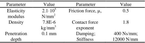
A mechanical design of a proposed exoskeleton is represented in Fig. 12. The structure has to be designed to permit adjustments of mechanism links in accordance with different human body constitution. A dynamic simulation has been developed by using a proper model for operation tests in ADAMS environment (Adams 2017). Contact, stiffness, damping coefficients, and friction force coefficients have been defined accordingly as listed in Table I with links made of steel.
[image:4.595.49.286.423.726.2]The exoskeleton consists of two mechanisms for the left and right legs. The legs are composed of 7 elements connected by 10 kinematic rotating joints. The electric motor with reducer (9), which is mounted on the upper frame (10), is used to drive the two mechanisms.
Fig. 12. Exoskeleton design model in SolidWorks.
7
6 5
4
9 10
[image:4.595.313.541.472.693.2]Fig. 13. Detail of the exoskeleton upper part.
By means of a chain wheel drive transmission, the movement is transmitted to the shaft (11), which is mounted on the upper frame (10) by means of radial-axial ball bearing bearings. The motor elements (1) of the two leg mechanisms are connected to the drive shaft (11) and are oriented to 180 degrees. On the upper frame, the elements (2) and (7) are connected by means of the rotation joints (with bolts) E and F. The element (6) consists of two segments (HI) and (IM) mounted (welded) at an angle of 180 degrees. The exoskeleton has a human foot-like structure: the joint (F) represents the hip joint, the joint (H) represents the knee joint and the (FH) and the (HM) segments represent the femur and the tibia.
TABLE I
ADAMS PARAMETERS FOR DYNAMIC SIMULATION
Parameter Value Parameter Value
Elasticity modulus
2.1·105
N/mm2
Friction force, µs 0.5
Density 7.8E-6 kg/mm3
Contact force exponent
1.8 Penetration
depth
0.1 mm Damping; Stiffness
400 Ns/mm; 12000 N/mm
[image:5.595.304.549.54.245.2]Dynamic model with proper joints and foot-ground contact is presented in Fig. 14. Computed exoskeleton walking sequences are represented in Fig. 16 and main kinematic results are shown in Figs. 17 - 20. From Figs. 19 and 20 it can be remarked that appropriate values are obtained as compared with those from experimental tests and numerical kinematic analysis.
[image:5.595.305.548.269.434.2]Fig. 14. Exoskeleton dynamic model in ADAMS.
Fig. 15. Computed exoskeleton foot path trajectory.
Fig. 16. A walking frames in ADAMS simulation of the exoskeleton.
Fig. 17. Computed foot translational displacement.
[image:5.595.49.289.423.494.2] [image:5.595.304.550.466.690.2] [image:5.595.49.275.597.775.2]Fig. 18. Computed angular variation of knee and hip joints.
Fig. 19. Computed angular variation of knee and hip joints.
Fig. 20. Computed angular variation of knee and hip joints.
VI. CONCLUSIONS
A new prototype of a motion assistance and rehabilitation exoskeleton for human is developed with low cost and easy-operation features. Simulation results obtained with ADAMS computational model have reveal suitable performance for operation in walking rehabilitation application, although its design may require additional improvements in future developments, such the foot shape optimization. The proposed design is simple wearable and light with anthropomorphic structure. It operates with only one motor that can be controlled as concerns the angular velocity. The exoskeleton purpose is to fully help or partially assist human walking and assure proper gait rehabilitation.
REFERENCES
[1] B. Chen, et al.: Recent developments and challenges of lower extremity exoskeletons. Journal of Orthopaedic Translation, 2016, 5: 26-37.
[2] K. Anama, A.A. Al-Jumaily, Active exoskeleton control systems: state of the art. Procedia Eng. 41, 988–994 (2012)
[3] I. Díaz, J.J. Gil, E. Sánchez, Lower-limb robotic rehabilitation: literature review and challenges. J. Robot. (2011)
[4] T. Yan, et al., “Review of assistive strategies in powered lower-limb orthoses and exoskeletons”. Robotics and Autonomous Systems, 2015, 64: 120-136.
[5] W. Huo, et al., “Lower limb wearable robots for assistance and rehabilitation: A state of the art”. IEEE systems Journal, 2016, 10.3: 1068-1081.
[6] Dumitru N., Copilusi C., Geonea I., Tarnita D., Dumitrache I. (2015) Dynamic Analysis of an Exoskeleton New Ankle Joint Mechanism. In: Flores P., Viadero F. (eds) New Trends in Mechanism and
Machine Science. Mechanisms and Machine Science, vol 24.
Springer, Cham.
[7] I. Geonea, M. Ceccarelli, G. Carbone, Design and Analysis of an Exoskeleton for People with Motor Disabilities. The 14th IFToMM
World Congress, Taipei, Taiwan, 2015.
[8] Geonea, I. D. and Tarnita, D., Design and evaluation of a new exoskeleton for gait rehabilitation, Mech. Sci., 8, 307-321, https://doi.org/10.5194/ms-8-307-2017, 2017.
[9] I. Geonea et al., "New Assistive Device for People with Motor Disabilities", Applied Mechanics and Materials, Vol. 772, pp. 574-579, 2015.
[10] Geonea, I., Tarnita, D., Carbone, G., & Ceccarelli, M. (2019). Design and Simulation of a Leg Exoskeleton Linkage for Human Motion Assistance. In New Trends in Medical and Service Robotics (pp. 93-100). Springer, Cham.
[image:6.595.47.292.556.770.2]