Abstract— Logistics networks configuration is such kind of
problems concerning facility location, production and distribution planning along the whole process of material flow. Abundant research has been done in this field from modeling by considering different scenarios to methods such as different heuristic methods. However, the models do not consider the influence of the important postponement strategy on logistics networks in the era of mass customization. Furthermore, the multi-commodity models till now do not consider the influence of commonality among products. In this paper, a logistics network model considering product commonality and postponement is formulated. This model is expected to be used to analyze the impacts of commonality and postponement strategies on location-allocation decisions in logistics network planning.
Index Terms—logistics network design, location allocation,
supply chain, commonality, postponement.
I. INTRODUCTION
In the environment of global economy, enterprises must configure and utilize worldwide resources to keep the advantages of competition. How to source products from the most appropriate manufacturing facility, how to keep the balance between inventory, transportation and manufacturing costs, and how to match supply and demand under uncertainty are concerned by each company, especially the multinational companies [1]. It is impossible to realize the strategic goal without a well developed and realizable logistics system. High efficient international logistics system will become the core competence for an enterprise to control cost, reach high-level customer service, and hence realize global business successfully.
The importance of logistics network design, and the need for the coordination of production and distribution decisions, has long been evident. Facility location, as the decision at the strategic level in logistics system, plays an important role. Some strategic decisions concerned by facility location include selecting the right suppliers, determining the appropriate number of facilities such as plants and warehouses, determining the location of each facility, determining the size of each facility, determining sourcing
Manuscript received May 7, 2009.
Prof. Dr.-Ing. L. Schulze: Head of Department Planning and Controlling of Warehouse and Transport Systems (PSLT), Leibniz University Hannover, Germany (phone: +49 511 762-4885; fax: +49 511 762-3005; e-mail: [email protected]).
Dr. L. Li: Research assistant, Department Planning and Controlling of Warehouse and Transport Systems, Leibniz University Hannover, Germany (e-mail: [email protected]).
requirements, i.e., assigning activities to the facilities, determining distribution strategies, i.e., the flows of raw materials and finished products in the network. The objective of design or reconfiguration of the logistics network is to minimize annual system wide cost subject to a variety of service level requirements.
Abundant researches have been done to identify different location-allocation problems, ranging from the so-called p-median problem to uncapacitated facility location problem and capacitated facility location problem, to the versions considering dynamic and stochastic properties of the supply chain network, multiple products, and/or multiple layers/echelons with or without intra-layer flows, to some models integrating tactical and operational decisions in the logistics system, like production decisions, inventory management, and routing, to some models considering risk management, financial aspects, and international factors, etc. Correspondingly, models and different heuristics methods have been investigated.
As we all know that under the paradigms of mass customization, many companies have been modifying their supply chain with considering the strategies like commonality and postponement. However, in the location-allocation models, these two strategies have not yet been considered.
Commonality reflects the sharing degree of the products within a product family which is essential for economies of scale for the company. The sharing refers to common features or attributes in either the product or the manufacturing process for a set of products [2]. The commonality can reduce the overall inventory cost by reallocating inventories to upstream stages towards raw materials [3]. When inventory decisions are integrated with facility location decisions, the commonality strategy has to be considered as one factor in facility location decision making when incorporating inventory decisions simultaneously.
Postponement is another issue to be highlighted, which has also been emphasized in the review article [4]. The strategy of postponement means that the differentiation point of a product will be skipped to the end of the production process. The later the postponement point is sited in a process, the lower is the cost of providing variety. Boone et al. give a detailed portray of the evolution of postponement as a supply chain concept in supply chain management [5]. They addressed the challenges of extending postponement research beyond the manufacturing context. Schulze et al. have discussed the logistics management issues and strategies when products are individualized in the later stage of supply chain [6]. It is implemented only during the processes in the whole logistics network which can not produce interest.
A Logistics Network Model for Postponement
Supply Chain
This paper concerns such kind of logistics networks which distribute a family of products with different levels of commonality. Furthermore, it is allowed to adopt postponement in the supply chain. That is to say, partial production can be moved from plants to distribution centers. Consequentially, transportation activities may happen between suppliers and distributors. The problem of location-allocation considering commonality and postponement are identified and described in this paper, together with the developed model.
The rest of the paper is organized as follows. Section 2 describes the location-allocation problem in logistics network planning for product family with commonality and postponement. Section 3 introduces the models for such problem. Section 4 concludes the paper by identifying the future work, especially the potential solution techniques for the new model.
II. LITERATURE REVIEW
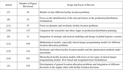
Since from time to time, there are quite some review papers in the field of location-allocation, we summarizes the main review papers in the literature in chronological order, as shown in Table I. Although these papers review the same field, i.e., location-allocation, they present different models and methods for different facility location problems from different aspects.
An early review was given in [7]. This paper clearly summarized the models of nine different facility location problems. Klose and Drexl reviewed further the papers from the mathematical modelling viewpoint and categorized the research into continuous location models, network location models, and mixed-integer programming models [8].
Goetschalckx et al. reviewed the mixed integer programming models of location-allocation problems as the foundation, and then focused on the identification of relevant factors included in the formulations, such as stochastic feature, dynamic characteristics, and status of facilities [9]. Erenguec et al. reviewed mainly the researches of facility location problems which integrated production decisions. The authors reported the decisions and models of the three stages, namely supplier stage, plant stage, and distribution stage in production/distribution planning [10].
Owen and Daskin reported on literature which explicitly addresses the stochastic and dynamic characteristics of facility location problems with a wide range of model formations and solution approaches [11]. Dynamic formulations focus on the difficult timing issues involved in locating facilities over an extended horizon. Stochastic formulations attempt to capture the uncertainty in problem input parameters such as forecast demand or distance values. Snzder did recently another survey regarding the inclusion of stochastic features in facility location models [12]. The paper mainly illustrated how optimization approaches cam be applied under uncertainty and the applications to facility location problems.
[image:2.595.49.547.493.777.2]Vidal and Goetschalckx summarized the basic international features and factors to be considered for model formulation in the existing literature [13]. Based on this categorization, Goetschalckx et al. expanded the characteristics of the logistics models from the international viewpoint [9]. Sahin and Süral focused on the hierarchical facility location models. They classified the problems based on flow pattern, service availability at each level of the hierarchy, and spatial configuration of services in addition to the objectives to locate facilities [14].
Table I: Review papers on location-allocation problem
Article Number of Papers
Reviewed Scope and Focus of Review
[7] 45 Models of nine different facility location problems
[8] 52 Focus on the identification of the relevant factors in the production/distribution formulations
[11] 97 Focus on dynamic and stochastic facility location problems
[10] 115 Categorize the researches into three stages in production/distribution planning [9] 31 Integration of strategic and tactical modeling and design of global logistics systems
[13] 199 Mathematical models, especially mixed integer programming models for different location-allocation problems
[12] 142 Stochastic and robust facility location models and the optimization methods under uncertainty
[14] 107 Hierarchical facility location models with focus on two types of mixed integer programming models: flow-based and assignment-base formulations
The latest review was done by Melo et al., which covered a big range of papers in the literature [4]. This article presented a refined review of the development of general location-allocation problems and a comprehensive introduction of properties and decisions of location-allocation problems from different aspects of supply chain, such as inventory, production, and routing, etc. Reverse logistics was emphasized since this topic has been receiving more attention. Solution techniques from the literature were also summarized.
III. PROBLEM IDENTIFICATION
In this section, the location-allocation problem with considering commonality and postponement strategies in the logistics network is described. To formulate the problem, it is firstly required to present in which way the commonality and postponement strategies are used.
Swaminathan and Tayur analyzed the final assembly process problem with an example which incorporates commonality and postponement. In the example, management decided to pilot an assembly process based on semi-finished products called vanilla boxes [15]. Fig. 1 shows the fictitious product family with three products f1, f2, and f3 made of four components a, b, c, and d.
f1 (a,b,c)
f2 (b,c,d)
f3 (a,c,d) Products:
Components:
a b c d
Product Family
Examples of Vanilla boxes
Vanilla box v1 containing (b, c) supports (f1, f2)
[image:3.595.48.286.369.559.2]Vanilla box v2 containing (c, d) supports (f2, f3)
Fig. 1: Product Family
The bills of material for the products are f1 = (a, b, c), f2 = (b, c, d), and f3 = (a, b, d). These products share more or less the same components with one another. For example, f1 and f2 both have the components b and c. V1, V2, and V3 are examples of feasible for the three products. V1 can be used in the assembly of f1 and f3 because these products can be assembled from it, by adding appropriate components. Thus a vanilla assembly process enabled assembly of customized products within much shorter lead times. To achieve this, though, the manufacturer had to carry additional inventory of vanilla boxes. However, in addition to the intermediate vanilla boxes form, the vanilla boxes are extremely allowed to be in the forms as components and as finished products. That is to say, there are multiple points of differentiation, in that there is no restriction on the type of vanilla box that can be stored as inventory. In general, when a customer order comes in, the product may be already ready, or produced by adding additional components to a vanilla box, or assembled directly
from all of the components.
Swaminathan and Tayur developed a stochastic integer program to determine the optimal types of vanilla boxes as well as their inventory levels [15]. They also explored the benefits of postponement through vanilla boxes under various settings. Among other results, they show that postponement using the intermediate form of vanilla boxes, i.e., semi-finished products outperforms both extreme forms of vanilla boxes as components or final products when the assembly capacity available is neither too slack nor too tight in the most real environments. However, in the model, the whole assembly or production process was piloted at one location. Hence, the decisions of which components should be present in the different vanilla boxes and how those vanilla boxes are allocated to the different products are used mainly to determine the time point to implement postponement strategy during the production process.
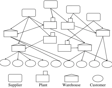
By extending the context of this example from production to production and distribution in the supply chain networks, we formulate the location-allocation problem with multiple products with sharing some common components, in multiple echelons by considering a supply chain like the one depicted by [16] with four main layers composed of suppliers, manufacturers, warehouses and distribution centers, and customers, as shown in Fig. 2.
[image:3.595.312.537.371.548.2]Supplier Plant Warehouse Customer
Fig. 2: General Logistics Network
products.
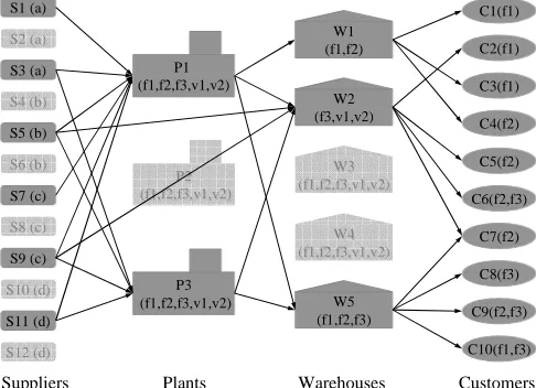
To better understand all of these decisions, we examine the hierarchical structure of a logistics network, as shown in Fig. 3. This is a 4-layer/echelon network for finally delivering the products shown in Fig. 1. Different icons are used to represent different potential facilities in the network, i.e., suppliers, plants, warehouses, and customers. Another point about the figure to be highlighted at first is that the icon in dark gray represents that the corresponding facility is selected in the network. Reversely, the icon in light gray means the corresponding facility is not selected in the network. This expression method reveals one kind of decisions to be made in logistics network design is what facilities to select. Another kind of decisions refers to the flows of the commodities from which origins to which destinations, shown in this figure as arrows.
S1 (a) C1(f1)
S2 (a) S3 (a)
S4 (b) S5 (b) S6 (b) S7 (c) S8 (c) S9 (c)
S10 (d) S11 (d) S12 (d)
Suppliers Plants Warehouses Customers
P3 (f1,f2,f3,v1,v2)
P3 (f1,f2,f3,v1,v2)
P2 (f1,f2,f3,v1,v2)
P2 (f1,f2,f3,v1,v2)
P1 (f1,f2,f3,v1,v2)
P1 (f1,f2,f3,v1,v2)
W1 (f1,f2)
W1 (f1,f2)
W2 (f3,v1,v2)
W2 (f3,v1,v2)
W3 (f1,f2,f3,v1,v2)
W3 (f1,f2,f3,v1,v2)
W4 (f1,f2,f3,v1,v2)
W4 (f1,f2,f3,v1,v2)
W5 (f1,f2,f3)
W5 (f1,f2,f3)
C2(f1)
C3(f1)
C4(f2)
C5(f2)
C6(f2,f3)
C7(f2)
C8(f3)
C9(f2,f3)
[image:4.595.47.290.262.438.2]C10(f1,f3)
Fig. 3: Hierarchical Structure of a Logistics Network The first layer includes twelve potential suppliers tagged from S1 to S12, represented by rounded rectangular icons. The letters in the brackets represent the components the suppliers can provide. For example, the potential suppliers S1, S2, and S3 have the component a, but S2 is not included in the network. Similarly, supplier S5 is selected to provide component b, while other two suppliers are excluded, and so on.
The second and the third layers represent the potential locations for facilities of plants and warehouses respectively with special icons. There are three potential plant locations tagged as P1, P2, and P3, and five potential warehouse locations from W1 to W5. Since the icons representing plant P2 and warehouses W3 and W4 are in light gray color, obviously, the three facilities are not included in the network.
The contents in the brackets in the light gray icons represent the potential products and vanilla boxes that can be produced in the corresponding facilities, while the contents in the dark gray icons represent the products and/or vanilla boxed that are finally determined to be produced in the corresponding facilities. In this case, the plant P1 is used to its total potential capability in manufacturing products f1, f2, and f3 and vanilla boxes v1 and v2 as well, while the warehouse W1 is only used to store final products f1 and f2, even though its potential capability can cover all the products and vanilla
boxes. It is easy to associate with the decision making of where to produce/store the products and vanilla boxes.
The forth layer undoubtedly corresponds to the customers tagged from C1 to C10 in elliptic icons. Which products are demanded by the customers is shown in the brackets in the elliptic icons. For example, the customer C1 requires product f1. As can be noticed from the figure, each ellipse is dark gray. That is to say, each customer should be satisfied. Of course, which customers are excluded in the service can also be a kind of decisions. But this is outside of the scope of our paper.
Although quantity information is not included in the figure, it is indeed necessary to make the decisions relating to quantities. Overall, the main decisions to be made in the location-allocation problem we consider are categorized and listed as follows:
1)Where to build the plants and warehouses?
2)Which suppliers to be selected for what kind of and how many components for the plants and warehouses? 3)What kinds of products and vanilla boxes and how many
are built in each plant?
4)What kinds of products and vanilla boxes and how many are built in each plant?
5)What kind of products and vanilla boxes and how many are transported from which plant to which warehouse?
IV. MODEL FORMULATION
For the problem described above, we developed the corresponding model. It is described as follows from the aspects of data sets, parameters, variables, constraints, and objectives.
A. Sets
S
: set of suppliers, indexed bys
.P
: set of potential locations for plants, indexed byp
.W
: set of potential locations for warehouses, indexed byw
.F
: set of products, indexed byf
.C
: set of customers, indexed byc
.R
: set of components, indexed byr
.V
: set of vanilla boxes, indexed byv
. fR
: set of components used in productf
. fV
: set of vanilla boxes used in productf
. fBV
: vanilla box included composition of productf
. rF
: set of products which need componentr
. rV
: set of vanilla boxes which need componentr
. vF
: set of products which need vanilla boxv
. rS
: subset of suppliers that can provide componentr
. fC
: set of customers which require productf
.V
R
F
K
=
∪
∪
: set of all commodities represented in the model, indexed byk
.k
P
: subset of plants at which commodityk
can be made. kW
: subset of warehouses at which commodityk
can be stored.W
P
S
C
W
P
D
=
∪
∪
: set of potential destinations for the commodities, indexed byd
.k
O
: set of potential origins for commodityk
. kD
: set of potential destinations for commodityk
. wF
: set of final products possible in warehousew
. The notations ofK
,O
, andD
are defined for notational convenience, with reference to [17] in their research. From the above definitions, we can getO
r=
S
r for any componentr
∈
R
,O
v=
P
v for any vanilla boxv
∈
V
, andO
f=
P
f∪
W
f for any productf
∈
F
. Similarly, possible destinations for a component r are plants at which products requiring this component can be made, i.e.,f F f r
P
D
=
∪
∈ r . Furthermore, possible destinations for avanilla box v are warehouses at which products requiring this vanilla box can be finally assembled, i.e.,
D
v=
∪
v∈FvW
f .Finally, the set of possible destinations for a product f is defined as
D
f=
W
f∪
C
fB. Parameters
rf
a
: quantity of componentr
required in the production of one unit of productf
.rv
b
: quantity of componentr
required in the production of one unit of vanilla boxv
.vf
c
: quantity of vanilla boxv
required in the production of one unit of productf
.f c
d
: demand of customerc
for productf
. oc
: fixed cost of selecting the origino
. ko
c
: operation cost of one unit of commodityk
at origino
. kod
c
: transportation cost of one unit of commodityk
from origino
to destinationd
.s
cs
: capacity of suppliers
. pcp
: capacity of plantp
. wcw
: capacity of warehousew
. vF
: total element number of the setF
v. oU
: middle parameter to represent if the origin is active, if0
=
oU
, yes. IfU
o=
1
, the origin is not active. ko
U
: middle parameter to represent the amount of commodityk
operated by origino
. kq
: lowest quantity of the commodity operated by one origin to have a discount for operation.k
l
: discount onc
ok, ifU
ok≥
q
k,0
≤
l
k≤
1
, ifU
ok<
q
k,1
=
k
l
.f
BV
n
: the number of the setsBV
f .C. Variables
k od
x
: quantity of commodityk
transported from the origino
to the destinationd
. wfv
y
: quantity of productf
which is produced from vanilla boxesv
in warehousew
,f
∈
F
w,
v
∈
V
f .In the models in the literature, the variables are quite often defined in three levels. The first level refers to binary variables. They are defined to represent which origin is selected for delivering a kind of commodity. For example, for each supplier, there is a binary variable to represent if the supplier is selected to deliver the material or not. Similarly, binary variables are defined for the potential locations of plants and warehouses. If the variable is equal to 1, normally, it means this location is selected to build a plant or warehouse. The second level means the variables which represent the quantity of commodities delivered from an origin or a destination in the network. The third level variables are used to represent the flow quantity of commodities between each possible pair of origin and destination.
Logically, it is very clear to define the three levels of variable. However, the activities of the second and third levels variables are dynamic during the optimization. They are not always active and can be assigned values. At first, the activity of the second level variables depends on the value of the first level variables. Furthermore, the activity of the third level variables depends on the value of the second level variables. Of course, indirectly, the first level variables control the activity of the third level variables. For example, if the variable for a supplier is equal to 0, that means this supplier is not selected to deliver the material. Hence, the variable at the second level representing the quantity delivered by this supplier is not active. Subsequently, the variable at the third level representing the flow quantity from this supplier as the origin can not be active either.
To solve the problem induced by the variables in three levels, conditional constraints are added to ensure that the higher level variables can not be assigned value. In this paper, we release such constraints by using only the third level variables. These variables can implicitly represent which origin is selected to deliver which commodity and the quantity, by calculating
U
o andU
ok through the functions∑ ∑
∈ ∈
=
K k d D
k od
o
x
U
, and∑
∈
=
D d
k od k
o
x
U
.1
=
f
BV
n
, then there is only one variable, and this variable can be directly equal to the difference of output and input.When the vanilla boxes in the warehouses are the same, we need to find out the optimal quantity for each product that can be produced from the same vanilla box. On the other hand, if the vanilla box can be used only for one product, then this variable is directly equal to the quantity of the product that can be produced from all of the vanilla boxes inputted into the warehouse. D. Constraints f W w f c f
wc
d
f
F
c
C
x
∑
∈∈
∈
=
−
0
,
,
(1)
R
r
W
w
x
a
x
b
x
a
x
f r r r C c f wc rf V v p Pv pw rv
F f p P
f pw rf S s r sw
∈
∈
=
−
+
+
∑
∑ ∑
∑ ∑
∑
∈ ∪ ∈ ∈ ∈ ∈,
,
0
(2),
,
f f Cc p P
f pw f wc F f w fv
V
v
W
w
x
x
y
f f w∈
∈
−
=
∑
∑
∑
∈ ∈∈ (3)
f f F f w fv rf S s r sw
R
r
W
w
y
a
x
w r∈
∈
=
−
∑
∑
∈ ∈,
,
0
/
(4),
,
0
/
f f F f w fv vf P p v pwV
v
W
w
y
c
x
w v∈
∈
=
−
∑
∑
∈∈ (5)
S
s
cs
x
x
s W w r sw P p rsp
+
∑
≤
∈
∑
∈ ∈
,
(6)P
p
cp
n
c
x
x
F pF f
vf
V v wW
v pw F
f wW f pw v v
∈
≤
+
∑ ∑
∑
∑ ∑
∈ ∈ ∈ ∈ ∈,
)
/
/(
(7)W
w
cw
x
w F f cCf wc f
∈
≤
∑ ∑
∈ ∈,
(8)Constraints (1) ensure that customer demands are satisfied by the warehouses. Constraints (2) ensure that the total amount of component r shipped to plant p is equal to the total amount required by all vanilla boxes and products made at this plant. Constraints (3) ensure the input of a product into a warehouse is equal to the output of the product from the warehouse. Constraints (4) and (5) ensure that the input components and vanilla boxes are finally used for the final products. All of the three constraints ensure that all finished products, vanilla boxes, and components that enter a warehouse also leave that warehouse. Constraints (6), (7), and (8) are the capacity constraints for suppliers, plants, and warehouses respectively.
E. Objective Function
]
)
(
[
min.
∑
∑
∑
∈ ∈ ∈
+
+
O
o k K d D
k od k od k o k o o
o
U
c
U
c
x
c
(9)The objective function (9) minimizes the sum of all fixed and variable costs.
V. CONCLUSIONS
This paper has summarized the development of logistics networks planning by analyzing the review papers in the literature. From the study, the research gap is identified. A new location-allocation model is formulated with considering the commonality among the products and postponement strategies in the logistics networks. The model can be used to make not only the general facility location decisions, like where to build the plant or warehouse, the allocation of commodities, but also the decisions on where to build the final products and vanilla boxes in the plants or warehouses.
Based on the proposed new location-allocation problem and model, further researches are to develop the method for solving such problems. Some mathematical optimization techniques have been widely adopted. Exact algorithms are used to find the optimal solutions, and heuristics are used to find good, but no necessarily optimal solutions. Simulation models are also well-known with the mechanism to evaluate specified design alternatives created by the designer.
Furthermore, some management issues and hints can be obtained by analyzing and comparing the results among the models with different scenarios, namely the models with only considering commonality or postponement, with considering both commonality and postponement, and without considering commonality and postponement.
Finally, one issue must be highlighted. Since the original emphasis of the paper is to discover the influence of commonality and postponement strategies on location-allocation decisions in logistics system planning, the basic model does not include uncertainty and time-period. However, considering that the spirit of commonality and postponement is to reduce the uncertainty of customer demand, the model would be more practical if it is extended for dynamic and stochastic logistics network scenarios.
REFERENCES
[1]D. Simchi-Levi, P. Kaminsky, and E. Simchi-Levi, Designing and Managing the Supply Chain: Concepts, Strategies, and Case Studies. New York: McGraw-Hill/Irwin, 2008.
[2]T. W. Simpson, J. R. A. Maier, and F. Mistree, "Product platform design: method and application," Research in Engineering Design, 13(1), 2001, pp.2-22.
[3]G. Q. Huang, X. Y. Zhang, and L. Liang, "Towards integrated optimal configuration of platform products, manufacturing processes, and supply chains," Journal of Operations Management, 23, 2005, pp.267-290.
[4]M. T. Melo, S. Nickel, and F. Saldanha-da-Gama, "Facility location and supply chain management – A review," European Journal of Operational Research, 2008, pp.1-12.
[6]L. Schulze, M. Gerasch, S. Mansky, and L. Li, "Logistics management of late product individualisation - application in the automotive industry," International Journal of Logistics Economics and Globalization, 1(3/4), 2008, pp. 330-342.
[7]C. H. Aikens, "Facility location models for distribution planning," European Journal of Operational Research, 22, 1985, pp.263-279. [8]A. Klose, and A. Drexl, "Facility location models for distribution system
design," European Journal of Operational Research, 162, 2005, pp.4-29.
[9]M. Goetschalckx, C. J. Vidal, and K. Dogan, "Modeling and design of global logistics systems: A review of integrated strategic and tactical models and design algorithms," European Journal of Operational Research, 143, 2002, pp.1-16.
[10] S. S. Erenguec, N. C. Simpson, and A. J. Vakharia, "Integrated production/distribution planning in supply chains: An invited review " European Journal of Operational Research, 115, 1999, pp.219-236. [11] S. H. Owen, and M. S. Daskin, "Strategic facility location: A review,"
European Journal of Operational Research, 111(3), 1998, pp. 423-447. [12] L. V. Snzder, "Facility location under uncertainty: a review," IIE
Transactions, 38, 2006, pp.537-554.
[13] C. J. Vidal, and M. Goetschalckx, "Strategic production-distribution models: a critical review with emphasis on global supply chain models," European Journal of Operational Research, 98, 1997, pp.1-18.
[14] G. Sahin, and H. Süral, "A review of hierarchical facility location models," Computers & Operations Research, 34, 2007, pp.2310-2331. [15] J. M. Swaminathan, and S. R. Tayur, "Managing broader product lines through delayed differentiation using vanilla boxes," Management Science, 44(12), 1998, pp.161-172.
[16] P. N. Thanh, N. Bostel, and O. Peton, "A dynamic model for facility location in the design of complex supply chains," International Journal of Production Economics, 113, 2008, pp.678-693.