Simulation Analysis of Prioritization Errors in the
AHP and Their Relationship with an Adopted
Judgement Scale
Andrzej Z. Grzybowski,
Member, IAENG,
Tomasz Starczewski
Abstract—The principal aim of the multiple-criteria decision analysis is the prioritization of available alternatives. This conventionally is achieved by estimation of the priority weights that reflect the importance of each of the alternatives. One of the most popular prioritization methodologies is the Analytic Hierarchy Process. The prioritization technics that can be used within this decision making framework are based on the so-called pairwise comparison matrix (PCM). The PCM contains the decision maker’s judgments about the priority-weights-ratios. These judgments are typically expressed in values from an adopted scale. In praxis such judgments are erroneous and as such, result in erroneous estimates of the priority weights. This paper is devoted to the simulation analysis of the estimation errors and their relationship with the correctness of the final ranking of alternatives. On the basis of the simulations’ results some important remarks about the impact of the adopted scale on the estimation errors as well as about the PCM acceptance procedure are formulated.
Index Terms—AHP, prioritization, estimation errors, consis-tency, simulation.
I. INTRODUCTION
M
ULtiple-criteria decision analysis (MCDA) is a branch of multiple criteria decision making that deals with problems that have only a small number of alternatives. The essence of the MCDA is the alternatives’ ranking creation also called a prioritization. The prioritization is achieved by estimation of the priority weights i.e. numbers telling to what degree a given alternative satisfies a given criterion. Apart from the alternatives and a number of criteria, more complex MCDA problems may also involve several experts and/or decision makers (DM). To obtain the final ranking of the available alternatives all these factors need to be ranked. One of the most popular prioritization method-ologies is the Analytic Hierarchy Process (AHP), [15]. In the AHP all problem’s factors are arranged in a hierarchic structure descending from - say - experts to criteria and alternatives in successive levels. After all sub-problems of prioritization are solved (i.e. the rakings of experts, criteria and alternatives are obtained), the final alternatives’ ranking is created. The prioritization technics that can be used within this decision making framework are based on the so-called pairwise comparison matrix (PCM). The PCM contains the decision maker’s judgments about the priority-weights-ratios. These judgments are typically expressed in values from an adopted predefined set of numbers that is called a scale, [14],Manuscript received 02.07.2018; revised 25.07.2018
A.Z. Grzybowski and T. Starczewski are with the Institue of Mathemat-ics, Faculty of Mechanical Engineering and Computer Science, Czesto-chowa University of Technology, CzestoCzesto-chowa, 42-201 Poland, e-mail: [email protected], [email protected]
[15], [3], [6], [18]. However in praxis the DM’s judgments are usually erroneous and as a consequence, the estimates of the priority weights derived on their basis are erroneous as well.
This paper is devoted to the simulation analysis of the priority-weights-estimation-errors (PWEEs) and their rela-tionship with the correctness of the final ranking of alter-natives. In Section 2 necessary definitions and facts from the theory are introduced. In Section 3 the problem is formally stated. Section 4 describes considered simulation frameworks and provides us with the results of simulation experiments along with discussion. Finally some concluding remarks about the impact of the adopted scale as well as about the PCM acceptance procedure are formulated.
II. PRELIMINARIES:NOTATION,DEFINITIONS AND BASIC FACTS
A basic assumptions of the AHP is the existence of a unique (up to multiplying constant) vector of priority weights v = (v1, . . . , vn)0 of n alternatives with respect to a given
criterion. Commonly the priority weights vi, i = 1, . . . , n,
are chosen to be nonnegative and normalized to unity. Such a vector is called a priority vector (PV) In the AHP a decision-maker evaluates ratios of prioritiesaij =vi/vj . As a result
the pairwise comparison matrix A = [aij]nxn is obtained.
Typically, the input data of the PCM is collected for the upper triangle of the matrixA, while the remaining elements are computed as the inverses of the corresponding symmetric elements in the upper triangle i.e.aij = 1/aji. Such a PCM
is said to bereciprocal. The PCM is said to beconsistentif it is reciprocal and its elements satisfy the condition:aijajk=
aik∀i, j, k= 1, ..., n.
However, it is obvious that in praxis it cannot be expected that the elements of PCM give precisely the priority ratios. First of all, according the usual procedure, the DM’s answers (given in lexical phrases) are transformed into numbers belonging to a given scale. In such a case one cannot neglect rounding errors. The most popular scale is the Saaty’s one (SS). The SS contains integers 1, 2, ..., 9 and their recip-rocals. Other suggested in literature scales are the Extended Saaty’s scale, ESS[N], that contains integers from 1 to N, along with their reciprocals, and the geometric scale GS[c] that contains numbers s of the form s = ci/2, i ∈ I with I being a predefined set of integers. For the analysis of the scales see e.g. [6], [18].
PCM in reality is inconsistent. So, an important problem connected with this theory is how to measure the degree of inconsistence of the PCM. But before we briefly introduce some inconsistency indices, first we need to recall two most popular prioritization methods. One of them is the so-called logarithmic least squares method, also known as geometric mean method - GM, [5]. The estimated priority vector (EPV) in the GM can be obtained by the following formula:
wi= n
Y
i=1 aij
!1/n .Xn
i=1
n
Y
i=1 aij
!1/n
Another, perhaps the most commonly used prioritization method is based on specific results from the spectral theory of matrices. This one is called right eigenvector method (REV). Its description and formal backgrounds have a vast literature, see e.g. [15], [16] and many contemporary books devoted to the AHP, so the details are omitted here to save the article space. In the REV as the EPV we take the eigenvector associated with the principal eigenvalue of the PCM at hand. It was indicated in literature, e.g. [7], [4], [13], that the EPVs obtained with the help of the GM and REV differ very little, and there is no agreement which one is better. However, the EPV is certainly much more easy to compute via the GM, thus this method will be primarily used in our studies. As we indicated, apart from deriving priority vectors, another problem within the AHP methodology is how to measure the degree of inconsistence of the PCM. We are presented with a number of inconsistency indices and again, the two most popular ones are related to the two above introduced prioritization methods.
The index connected with the REV, denoted as SI, was proposed by Saaty and is defined as follows:
SI(n) = λmax−n n−1
Related to the geometric mean method index (GI) was proposed by Crawford and Williams[5], and was popularized by Aguaron and Moreno-Jimenez [1] in 2003. It is given by
GI(n) = 2 (n−1)(n−2)
X
i<j
log2(aijwi/wj)
Apart from these two indices there is third popular index that is based on the notion of the triad inconsistency. It was proposed by Koczkodaj [12]. Following him, for any different i, j, k ≤ n, a tuple (aik, aij, akj) will be called a triad.
Koczkodaj proposed to characterize the triad’s inconsistency by the number:
T I(aik, akj, aij) = min
1−aikakj/aij
,1−aij/((aikakj)
Then, the Koczkodaj’s inconsistency index KI of any reciprocal PCM is defined as a maximum of triad’s in-consistencies i.e. KI = max[T I(aik, akj, aij)], where the
maximum is taken over all triads in the upper triangle of the PCM. Yet another inconsistency index that manifests very good correlation with PV estimation quality was defined as the average value of all triad’s inconsistencies. It was introduced and studied in [8] and is denoted here as ATI.
All inconsistency indices are developed in order to enable the DM to distinguish between useful and useless PCMs. Thus, usually all these indices are given along with related
consistency thresholds. However, as it was criticized by many researchers, typically the values of acceptance thresholds are based on some heuristics and are not supported by any profound formal reasoning or statistical research. In recent literature there are many confusing examples that prove that the thresholds work poorly, see [7] and literature in there. To deal with this problem a new approach to PCM acceptance was proposed quite recently in [8], where the relationship between the inconsistency indices and the PWEEs was examined with the help of Monte Carlo simulations. In [8] it was proposed to measure the PWEE as the average absolute (AE) and/or relative (RE) errors. The errors are given by the following formulae:
AE(v,w) = 1 n
n
X
i=1
|vi−wi| (1)
RE(v,w) = 1 n
n
X
i=1
|vi−wi|
vi
(2)
wherev= (v1, ..., vn)is the true PV whilew= (w1, ..., wn)
is its EPV. Obviously the EPV and consequently the errors depend on the prioritization method as well. So, in our studies both the GM and REV were used for PV estimation and then calculation of AE and RE.
III. PROBLEMSTATEMENT
As we have mentioned above, it is argued that the knowl-edge about the relationship between inconsistency indices and PWEEs would help the DM in making decisions about the PCM acceptance because such decisions are based on the observed value of the inconsistency index. The principal aim of this paper is to help the DM in such a task. To achieve this goal one should be able to distinguish between ”small”, ”average” and ”big” PWEEs. However, as yet there are no criteria for making such a ”classification” of errors. To cope with the problem we propose here, for the first time in literature, to investigate the relationship between the PWEEs and the chances of ”significantly wrong” final EPV. The latter term as well as the idea of the proposed criterion needs additional clarification. Below we present more formal and more detailed description of our proposal.
During typical analysis of the AHP problem, both the prioritization methods and the inconsistency analysis are curried out several times (as described in Introduction, at least for the criteria and then at the bottom of the hierarchy, for the alternatives with respect to each criterion separately). Let the PCM(Cr) denote the PCM that was evaluated for the criteria, and let PCM(i) denote the PCMs for the alternatives with respect to i-th criterion. The PCM(Cr) has order k, wherekis the number of different criteria in the considered problem(k >1). The PCM(i) has the ordern, withnbeing, as previously, the number of available alternatives. Let v0 and w0 be, respectively, the true PV for criteria and the EPV computed for the criteria on the basis of PCM(Cr). Let also vi and wi be the true PV and its EPV for the
alternatives with respect to thei-th criterion. The true final ranking of the alternatives is given by the final true PV - say
v- that is computed as the weighted average of the vectors
vi, i= 1, , k, with the weights given inv0. Analogously, the
average of the vectorswi, i= 1, , k, with the weights given
inw0
We will say, thatw provides us with significantly wrong final ranking if the truly best alternative (i.e. the one asso-ciated with greatest coefficient in v) is not the best one in the final ranking (i.e. its corresponding coefficient in w is not the greatest one) Hereafter we will abbreviate the phrase ”significantly wrong final ranking” to SWFR.
We propose such a definition to focus only on serious mis-takes in rankings, so our criterion does not take into account such situations where the final classification is wrong, but the erroneous ranks are related to less significant alternatives. That is why we call it ”significantly wrong”.
From the multiple-criteria decision analysis point of view, not the PWEEs themselves but the chances for significantly wrong final ranking is perhaps the most important criterion for the PCM acceptance or rejection. So, the first aim of our studies is to find out what is the relationship between the magnitude of the PWEEs and the probabilities of obtaining SWFR.
Another interesting question is what type of error is more meaningful, the AE or RE? In [8] it was suggested that in the context of the AHP application the more important is the RE. However this statement was superted only by intuition and some heuristics. Now we want to study which of the two types of errors are better related to the probability of the SWFR.
Yet another problem considered in our studies is the classification of the PWEEs, as mentioned at the beginning of this section. We focus here on the class of ”small” errors. In our opinion, as such can be treated these errors that result from the methodology itself, that is the rounding errors. We study whether the magnitude of such ”small” errors depends on the adopted scale and - if so - which scale is the best one under the criterion of the SWFR.
All these questions can be answered only with the help of Monte Carlo simulation. Next section provides us with the description of the simulation frameworks that are used in our studies.
IV. SIMULATION FRAMEWORKS AND RESULTS
To analyze the relationship between the PWEEs and the probabilities of obtaining the SWFR we use the following simulation framework:
•
Step 0 (Initialization) Set: n - the number of alterna-tives, k- the number of criteria, N -the number of simulated AHP problems, P R- the probability distribution of random PV-estimation errors Step 1 Randomly generate the ”true” priority vectors
vi, i= 1, , k,
Step 2 According to theP R, compute ”estimated” priority vectors wi, i = 1, ..., k, as random modifications of corresponding true priority vectors.
Step 3 With the help of formulae 1 and 2 compute the PWEEs:Ai=AE(vi,wi)andRi=RE(vi,wi),
i= 0, , k.
Step 4 Compute the aggregated estimation errors as: AAE = 1/(k+ 1)Pk
i=0Ai andARE = 1/(k+
1)Pk
[image:3.595.327.525.105.156.2]i=0Ri
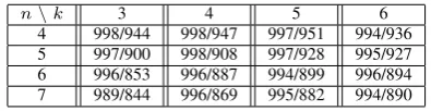
TABLE I: Values of Pearson correlation coefficients between the probabilities (frequencies) of SWFR and the mean values of AAE (first number) and ARE (second number). Only fractional digits are presented.
n\k 3 4 5 6
4 998/944 998/947 997/951 994/936
5 997/900 998/908 997/928 995/927
6 996/853 996/887 994/899 996/894
7 989/844 996/869 995/882 994/890
Step 5 Set sw= 1 if the true best alternative is different from the estimated best alternative, otherwise set sw= 0
Step 6 Write down all values computed and/or set in Steps 3 to 5 as one record.
Step 7 N times repeat Steps 1 to 6
Step 8 Return all records organized as one database. As a result of simulation experiments conducted within the above simulation framework we receive a database that enables us to study the relationship between the PWEEs and the probabilities of obtaining the SWFR. For this purpose the whole database is arranged in ascending order according the values of a considered type of errors (Ai, Ri, AAE or
ARE)and then split into a number (N C) of separate classes ECi, (i= 1, ..., N C). For each such a class the mean value
of the considered error is computed as well as the number of cases of the SWFR (i.e. computed within the given class ECi sum of the values of sw as recorded in Step 5). Fig
1 presents exemplary results obtained for problems where n= 4, k= 4, numeber of classes is N C= 35.
The plot (a) in Fig. 1 illustrates the relationship between the averages of aggregated absolute error AAE and the probabilities of SWFR, while the one labeled (b) shows the relationship between aggregated relative error ARE and the probabilities od SWFR. What is quite surprising, in difference to the suggestions in literature (see [[8]), the abso-lute errors manifest better correlation with the probabilities of SWFR. This shows that the heuristics underlying some conclusions may be sometimes misleading. The relationship presented in Fig 1 was obtained for the case where the number of alternatives as well as the number of criteria is 4. However the same relationship was observed for all other considered numbers of alternatives and criteria. In our studies we have considered n = 4, ...,7 and k = 3, ...,6. Table I shows values of the Pearson correlation coefficient obtained in all these cases. Column heads indicate number of criteria k, heads of rows indicate number of alternatives. To save the table space, in appropriate cells only fractional digits are presented.
We can see that that apparently both types of errors are strongly correlated with the probability of SWFR, and in that sense both are meaningful. However in all cases the correlation coefficient computed for the AAE is greater than the one in case of the ARE. So the results confirm our previous conclusion. Moreover, one can also notice that the correlation of ARE decreases when the number of alternatives increases, while the correlation of AAE is much more robust against such changes.
AE Pr
0.1 0.2
0.1 0.3 0.5 0.7
(a)
RE Pr
0.5 1. 1.5 2
0.2 0.4 0.6
[image:4.595.100.499.60.175.2](b)
Fig. 1: The relationship between the the probabilities (frequncies) of SWFR (lebeled as P r) and the AAE, plot (a), and ARE, plot (b). This exemplary graph was obtained in the case where n= 6, k = 3. The whole range of observed errors was splited intoN C = 35classes.
PWEEs such ones that are of similar magnitude as those resulting from the rounding procedure. So, our another task is to determine how small are the ”small” errors and what is their relationship with the adopted judgment scales. For this study we assume the following simulation framework:
•
Step 0 (Initialization) Set:n - the number of alternatives, k- the number of criteria,N -the number of simu-lated AHP problems, the prioritization method (GM or REV)
Step 1 Randomly generate the true priority vectorsvi, i=
1, ..., k, and compute related perfect comparison
matrixMi with elementsmij,l= v
i j
vi l
Step 2 For every considered judgment scale separately, compute rounded matrices RMi, i = 0, ..., k, by rounding all values in the upper triangle of
Mi, i= 0, ..., k, to the closest value from the scale
and replace all elements in the lower triangle of the RMi with the reciprocities of the appropriate
elements from the upper triangle.
Step 3 With the help of adopted prioritization method compute the values of the estimates of the vectors
vi, i= 1, ..., kalong with the errorsA
i, Ri, AAE
orARE. Write down values computed in this step as one record.
Step 4 N times repeat Steps 1 and 3
Step 5 Return all records organized as one database. In our studies we make use of the Saaty’s scale (SS), ExtendedSaaty’s scale ESS[17], and geometric scale GS[2], (their definitions were provided in Section 2). Results of our simulation studies are summerized in Table II
The rounding procedure is an immanent part of all pair-wise comparison judgments. As a result, the rounding errors cannot be avoided and have to be accepted. So it is natural to treat each error in judgment that has similar magnitude to the rounding error as a small one or even negligible. In our opinion the limit for this kind of errors should be given by the maximum of the observed rounding errors. If we accept this point, then we should notice that, in view of Table II the magnitude limit for small errors depends on the assumed judgment scale. And from this point of view the GS[2] and and EES[17] looks much better than the usual SS. Such a poor performance of the SS were also pointed out in other research conclusions, see e.g. [18].
Another important observation is that even such small errors may lead to SWPR! It another amazing fact revealed
TABLE II: Selected statistics for AA errors that are results of the rounding procedure in dependence on the adopted judgment scale. The considered scales are SS, ESS[17] and GS[2] as defined in Section 2.
Statistics Min Max Mean St. Deviat.
Scale: n
SS 4 0.0044 0.0360 0.01383 0.0038
SS 5 0.0048 0.0302 0.0125 0.0035
SS 6 0.0039 0.0286 0.0113 0.0032
SS 7 0.0041 0.0260 0.0101 0.0029
ESS[17] 4 0.0040 0.0245 0.0115 0.0028
ESS[17] 5 0.0038 0.0218 0.0100 0.0024
ESS[17] 6 0.0034 0.0187 0.0090 0.0021
ESS[17] 7 0.0033 0.0177 0.0079 0.0019
GS[2] 4 0.0032 0.0204 0.0085 0.0022
GS[2] 5 0.0027 0.0194 0.0074 0.0021
GS[2] 6 0.0025 0.0176 0.0066 0.0019
GS[2] 7 0.0021 0.0175 0.0059 0.0018
by presented here studies. If we, for example, take into account the relationship illustrated in Fig 1. we can see that AA errors of magnitude less that the limits for small errors are related to AHP problems where we have probability above 0.05 of SWFR. The results presented in Table II were obtained in simulations where the GM prioritization method was used to obtain the EPV. However, when we used the REV method the results were basically the same and they led to the same conclusions, so we omit their presentation to save the article space.
V. FINAL REMARKS
The simulation experiments described in this paper re-vealed interesting facts. First fact is that not the relative errors but the absolute errors are better correlated with the chances of significantly wrong final ranking. Second, that the small estimation errors - i.e. of magnitude similar to the rounding errors - are not negligible because they also may cause the change of order of the two most important alternatives, and the probability of such situation is between 5% and 8%. Next interesting observation is that adoption of the geometric scale (here the GS[2]) leads to smaller rounding errors than the extended Satty’s scale (here ESS[17]). The worst with respect to this criterion is the usual Saaty’s scale.
[image:4.595.315.537.292.425.2]a single prioritization problem (i.e. problem of estimating weights on the basis of a fixed and only one PCM), see e.g. as in [7], [9], [4], [13], [3], [19]. The approach adopted here to simulation analysis of AHP problems was introduced for the first time in [11]. However in the context of error analysis this approach is used for the first time in literature. What is very important, the relationship between the estimation errors and the chances of SWFR are much more vague when we consider the single prioritization problem.
The results should have impact on the PCM acceptance methodology. The impact should be at least twofold. First, we know when the PCM should be (or even has to be) accepted; when the AE errors (or RE errors) are small (as defined here). Secondly, the very close relationship between AE errors and the probability of significantly wrong final PV (as illustrated e.g. by by Fig. 1 or Table I) can form a sound fundament for development of a new PCM-acceptance procedure that would really on the analysis of the chances of good/ bad consequences of the decisions, and be well justified by the mathematical-statistics methodology.
Finally, let us note that the PWEEs (of both types) cannot be observed directly, but the values of inconsistency indices can be observed instead. The relationship between the values of inconsistency indices and the AE and RE errors where analyzed in [8]. It appears that the best correlation was found between the ATI index and the PWEEs of both types. More detailed discussion on this issue can be found in [8]. In view of presented here results further thorough studies within this area should be conducted in future. But in the light of presented results it is very promising direction.
REFERENCES
[1] J. Aguaron, J.M. Moreno-Jimenez, ”The geometric consistency index: Approximated thresholds”, Euro. J. Oper. Res. 147, 137-145, 2003. [2] J. Alonso, T. Lamata, ”Consistency in the Analytic Hierarchy Process:
a New Approach”, Inter. J.Uncertain., Fuzzin. Knowl.-Based Syst., 14, 445-459, 2006.
[3] D.V. Budescu, R. Zwick, A. Rapoport ”Comparison of the analytic hierarchy process and the geometric mean procedure for ratio scaling”, Appl. Psychol. Meas., 10, 69-78, 1986.
[4] E.U. Choo, W.C. Wedley, ” A common framework for deriving pref-erence values from pairwise comparison matrices”, Comp. Oper. Res. 31, 893-908, 2004.
[5] G. Crawford, C.A. Williams, ” A note on the analysis of subjective judgment matrices. J. Math. Psychol. 29, 387-405, 1985.
[6] Y. Dong, Y. Xu, H. Li, M. Dai, ”A comparative study of the numerical scales and the prioritization methods in AHP”, Euro. J. Oper. Res. 186, 229-242, 2008.
[7] A.Z. Grzybowski, ”Note on a new optimization based approach for estimating priority weights and related consistency index”, Expert Systems with Applications , 39, 11699-11708, 2012.
[8] A.Z. Grzybowski, ”New results on inconsistency indices and their relationship with the quality of priority vector estimation”, Expert Systems With Applications 43 197-212, 2016.
[9] A.Z. Grzybowski, T. Starczewski, ”Remarks about Inconsistency Anal-ysis in the Pairwise Comparison Technique”, Proceedings of IEEE 14th International Scientific Conference on Informatics, Poprad, (eds. Novitzka, S. Korecko, A. Szakal), pp.227-231, New York 2017. [10] P.T. Kazibudzki, ”Redefinition of triad’s inconsistency and its impact
on the consistency measurement of pairwise comparison matrix”, Jour-nal of Applied Mathematics and ComputatioJour-nal Mechanics, vol. 15, no. 1, pp. 71-78, 2016.
[11] P.T. Kazibudzki, A.Z. Grzybowski, ”On some advancements within certain multicriteria decision making support methodology”, American Journal of Business and Management, Vol. 2, No. 2, pp.143-154 2013. [12] W.W. Koczkodaj ”A new definition of consistency of pairwise com-parisons”, Mathematical and Computer Modelling 18(7), 79-84, 1993. [13] C-C Lin, ”A Revised Framework for Deriving Preference Values from Pairwise Comparison Matrices” Euro. J. Oper. Res., 176, 1145-1150, 2007.
[14] T.L. Saaty, ”Scaling method for priorities in hierarchical structures”, J. Math. Psychol., Vol. 15, No. 3, 234-281, 1977.
[15] T.L. Saaty, The Analytic Hierarchy Process, McGraw Hill, New York 1980.
[16] T.L. Saaty, L.G. Vargas, ”Comparison of eigenvalue, logarithmic least square and least square methods in estimating ratio”. J. Math. Model., 5, 309-324, 1984.
[17] T. Starczewski, ”Relationship between priority ratios disturbances and priority estimation errors”, Journal of Applied Mathematics and Computational Mechanics, 15(3), 143-154, 2016.
[18] T. Starczewski, ”Remarks on the impact of the adopted scale on the priority estimation quality”. Journal of Applied Mathematics and Computational Mechanics, 16(3), 105-116, 2017.