Missile Guidance & Control Systems pdf

(1)

(2)

(3)

(4)

George M. Siouris

Missile Guidance

(5)

Consultant

Avionics and Weapon Systems Formerly

Adjunct Professor

Air Force Institute of Technology

Department of Electrical and Computer Engineering Wright-Patterson AFB, OH 45433

USA

[email protected]

Cover illustration: Typical phases of a ballistic missile trajectory.

Library of Congress Cataloging-in-Publication Data Siouris, George M.

Missile guidance and control systems / George M. Siouris. p. cm.

Includes bibliographical references and index. ISBN 0-387-00726-1 (hc. : alk. paper)

1. Flight control. 2. Guidance systems (Flight) 3. Automatic pilot (Airplanes) I. Title. TL589.4.S5144 2003

629.132′6–dc21

2003044592 ISBN 0-387-00726-1 Printed on acid-free paper.

All rights reserved. This work may not be translated or copied in whole or in part without the written permission of the publisher (Springer-Verlag New York, Inc., 175 Fifth Avenue, New York, NY 10010, USA), except for brief excerpts in connection with reviews or scholarly analysis. Use in connection with any form of information storage and retrieval, electronic adaptation, computer software, or by similar or dissimilar methodology now known or hereafter developed is forbidden.

The use in this publication of trade names, trademarks, service marks, and similar terms, even if they are not identified as such, is not to be taken as an expression of opinion as to whether or not they are subject to proprietary rights.

Printed in the United States of America. TES/SBA 9 8 7 6 5 4 3 2 1 SPIN 109/8951

(6)

(7)

(8)

Preface

In every department of physical science there is only so much science, properly so-called, as there is mathematics.

Immanuel Kant Most air defense systems in use or under development today, employ homing guidance to effect intercept of the target. By virtue of the use of onboard data gathering, the homing guidance system provides continually improving quality of target information right up to the intercept point. More than any single device, the guided missile has shaped the aerospace forces of the world today. Combat aircraft, for example, are fitted with airborne weapons that can be launched against enemy aircraft, ground forces, or strategic targets deep inside enemy territory. Also, the guided missile can be employed as a diversionary weapon to confuse ground and air forces. Ground-based missile systems have various range capabilities from a few miles to several thousand miles. These ground-based missiles are ballistic or nonbal-listic types, depending on their mission requirements. The design of a guided weapon (i.e., a missile) is a large undertaking, requiring the team effort of many engineers having expertise in the areas of aerodynamics, flight controls, structures, and propul-sion, among others. The different design groups must work together to produce the most efficient weapon in terms of high accuracy and low cost.

(9)

of benefit to engineers engaged in the design and development of guided missiles and to aeronautical engineering students, as well as serving as a convenient reference for researchers in weapon system design.

The aerospace engineering field and its disciplines are undergoing a revolutionary change, albeit one that is difficult to secure great perspective on at the time of this writing. The author has done his best to present the state of the art in weapons systems. To this end, all criticism and suggestions for future improvement of the book are welcomed.

The book consists of seven chapters and several appendices. Chapter 1 presents a historical background of past and present guided missile systems and the evolu-tion of modern weapons. Chapter 2 discusses the generalized missile equaevolu-tions of motion. Among the topics discussed are generalized coordinate systems, rigid body equations of motion, D’Alembert’s principle, and Lagrange’s equations for rotat-ing coordinate systems. Chapter 3 covers aerodynamic forces and coefficients. Of interest here is the extensive treatment of aerodynamic forces and moments, the vari-ous types of missile seekers and their function in the guidance loop, autopilots, and control surface actuators. Chapter 4 treats the important subject of the various types of tactical guidance laws and/or techniques. The types of guidance laws discussed in some detail are homing guidance, command guidance, proportional navigation, augmented proportional navigation, and guidance laws using modern control and estimation theory. Chapter 5 deals with weapon delivery systems and techniques. Here the reader will find many topics not found in similar books. Among the numer-ous topics treated are weapon delivery requirements, the navigation/weapon delivery system, the fire control computer, accuracies in weapon delivery, and modern topics such as situational awareness/situation assessment. Chapter 6 is devoted to strate-gic missiles, including the classical two-body problem and Lambert’s theorem, the spherical Earth hit equation, explicit and implicit guidance techniques, atmospheric reentry, and ballistic missile intercept. Chapter 7 focuses on cruise missile theory and design. Much of the material in this chapter centers on the concepts of cruise missile navigation, the terrain contour matching concept, and the global positioning system. Each chapter contains references for further research and study. Several appendices provide added useful information for the reader. Appendix A lists several fundamental constants, Appendix B presents a glossary of terms found in technical publications and books, Appendix C gives a list of acronyms, Appendix D discusses the standard atmosphere, Appendix E presents the missile classification, Appendix F lists past and present missile systems, Appendix G summarizes the properties of conics that are useful in understanding the material of Chapter 6, Appendix H is a list of radar frequencies, and Appendix I presents a list of the most commonly needed conversion factors.

(10)

design, operation, and testing (i.e., from concept to fly-out) the air-launched cruise missile (ALCM),SRAM II,Minuteman III, theAIM-9 Sidewinder, and other programs too numerous to list.

Obviously, as anyone who has attempted it knows, writing a book is hardly a soli-tary activity. In writing this book, I owe thanks and acknowledgment to various people. For obvious reasons, I cannot acknowledge my indebtedness to all these people, and so I must necessarily limit my thanks to those who helped me directly in the preparation and checking of the material in this book. Therefore, I would like to acknowledge the advice and encouragement that I received from my good friend Dr. Guanrong Chen, formerly Professor of Electrical and Computer Engineering, University of Houston, Houston, Texas, and currently Chair Professor, Department of Electronic Engineering, City University of Hong Kong. In particular, I am thankful to Professor Chen for suggesting this book to Springer-Verlag New York and working hard to see that it received equitable consideration. Also, I would like to thank my good friend Dr. Victor A. Skormin, Professor, Department of Electrical Engineering, Thomas J. Watson School of Engineering and Applied Science, Binghamton University (SUNY), Binghamton, New York, for his encouragement in this effort. To Dr. Pravas R. Mahapatra, Professor, Department of Aerospace Engineering, Indian Institute of Science, Bangalore, India, I express my sincere thanks for his commitment and painstaking effort in reviewing Chapters 2– 4. His criticism and suggestions have been of great service to me. Much care has been devoted to the writing and proof-reading of the book, but for any errors that remain I assume responsibility, and I will be grateful to hear of these.

The author would like to express his appreciation to the editorial and production staff of Springer-Verlag New York, for their courteous cooperation in the production of this book and for the high standards of publishing, which they have set and maintained. Finally, but perhaps most importantly, I would like to thank my family for their forbearance, encouragement, and support in this endeavor.

Dayton, Ohio George M. Siouris

(11)

(12)

1 Introduction

Rockets have been used as early asA.D.1232, when the Chinese employed them as unguided missiles to repel the Mongol besiegers of the city of Pein-King (Peiping). Also, in the fifteenth century, Korea developed thesinkijon∗(orSin-Gi-Jeon) rocket. Manufactured from the early fifteenth to mid-sixteenth century, the sinkijon was actively deployed in the northern frontiers, playing a pivotal role in fending off inva-sions on numerous occainva-sions. Once out of the rocket launcher, the fire-arrows were set to detonate automatically near the target area. Also, the high-powered firearm was utilized in the southern provinces to thwart the Japanese marauders. The main body of thesinkijon’s rocket launcher was five to six meters long, the largest of its kind at that time∗∗_{. A}_sinkijon_{was capable of firing as many as one hundred fire-arrows} or explosive grenades. The fire-arrow contained a device equipped with gunpowder and shrapnel, timed to explode near the target. The introduction of gunpowder made possible the use of cannon and muskets that could fire projectiles great distances and with high velocities. It was desirable – in so far as the study of cannon fire is desirable – to learn the paths of these projectiles, their range, the heights they could reach, and the effect of muzzle velocity. Several years later, thesinkijonwent through another significant upgrade, which enabled it to hurl a fire-arrow made up of small warheads and programmed to detonate and shower multiple explosions around the enemy. In 1451, King Munjong ordered a drastic upgrade of the hwacha (a rocket launcher on a cartwheel). This improvement allowed as many as one hundred sinki-jons to be mounted on the hwacha, boosting the overall firepower and mobility of the rocket.

Since those early times and in one form or another, rockets have been used as weapons and machines of war, for amusement through their colorful aerial bursts, as life-saving equipment, and for communications or signals. The lack of suitable guid-ance and control systems may have accounted for the rocket’s slow improvement over the years. Strangely enough, it was the airplane rather than the rocket that stimulated the development of a guided missile as it is known today.

∗_Sinkijon_{means “ghost-like arrow machine.”}

∗∗_{The author would like to thank Dr. Jang Gyu Lee, Professor and Director of the}

(17)

In the twentieth century, the idea of using guided missiles came during World War I. Specifically, and as stated above, the use of the airplane as a military weapon gave rise to the idea of using remote-controlled aircraft to bomb targets. As early as 1913, René Lorin, a French engineer, proposed and patented the idea for a ramjet powerplant. In 1924, funds were allocated in the United States to develop a missile using radio control. Many moderately successful flights were made during the 1920s with this control, but by 1932 the project was closed because of luck of funds. Radio-controlled target planes were the first airborne remote-Radio-controlled aircraft used by the Army and Navy.

Dr. Robert H. Goddard was largely responsible for the interest in rockets back in the 1920s. Early in his experiments he found that solid-propellant rockets would not give him the high power or duration of power needed for a dependable supersonic motor capable of extreme altitudes. On March 16, 1926, Dr. Goddard successfully fired the first liquid-propellant rocket, which attained an altitude of 184 ft (56 m) and a speed of 60 mph (97 km/hr). Later, Dr. Goddard was the first to fire a rocket that reached a speed faster than the speed of sound. Moreover, he was the first to develop a gyroscopic steering apparatus for rockets, first to use vanes in the jet stream for rocket stabilization during the initial phase of a rocket in flight, and the first to patent the idea of step rockets.

The first flight of a liquid-propellant rocket in Europe occurred in Germany on 14 March 1931. In 1932 Captain Walter Dornberger (later a general) of the German Army obtained the necessary approval to develop liquid-propellant rockets for military purposes [1]. Subsequently, by 1936 Germany decided to make research and development of guided missiles a major project, known as the “Peenemünde Project,” at Peenemünde, Germany. The German developments in the field of guided missiles during World War II were the most advanced of their time. Their most widely known missiles were theV-1andV-2surface-to-air missiles (note that the designation V1and/orV2is also found in the literature). As early as the spring of 1942, the original V-1had been developed and flight-tested at Peenemünde.

In essence, then, modern weapon (missile) guidance technology can be said to have originated during World War II in Germany with the development of the V-1andV-2(German: A-4; the A-4stands for Aggregat-4, or fourth model in the development type series; theV stands forVergeltungswaffe, or retaliation weapon, while some authors claim that initially, it stood forVersuchsmuster or experimental model) surface-to-surface missiles by a group of engineers and scientists at Peen-emünde. It should be noted that static firing of rockets, notably the A-3, was per-formed as early as in the spring of 1936 at the Experimental Station, Kummersdorf West (about 17 miles south of Berlin). In the spring of 1942 the originalV-1(also known by various names such asbuzz bomb, robot bomb, flying bomb, air torpedo, orFieseler Fi-103) had been developed and flight-tested at Peenemünde. Thus, the V-1andV-2ushered in a new type of warfare employing remote bombing by pilotless weapons launched over a hundred miles away through all kinds of weather, day and night [1], [3].

(18)

from an inclined concrete ramp 45.72 m (150 ft) long and 4.88 m (16 ft) above the ground at the highest end, theV-1flew a preset distance, and then switched on a release system, which deflected the elevators, diving the missile straight into the ground. The engine was capable of propelling theV-1724 km/hr (450 mph). A speed of 322 km/hr (200 mph) had to be reached before theV-1propulsion unit could maintain the missile in flight. The range of theV-1was 370 km (230 miles). Guidance was accomplished by an autopilot along a preset path. Specifically, the plane’s (or missile’s) course stabilization was maintained by a magnetically controlled gyroscope that directed a tail rudder. When the predetermined distance was reached, as mentioned above, a servomechanism depressed the elevators, sending the plane into a steep dive. TheV-1 was not accurate, and it was susceptible to destruction by antiaircraft fire and aircraft. Several versions of theV-1were developed in Germany at that time. One version was designed for launch from the air. The missile could be carried under the left wing

of aHeinkel He-111aircraft. Amanned V-1version was also developed, called the

Reichenberg, flown first by Willy Fiedler, followed by Hanna Reitch. This version was planned for suicide missions. Three versions were built.

(19)

theV-2system was the first primitive example of inertial guidance, making use of gyroscopes and accelerometers [3].

Several other German missiles were also highly developed during World War II and were in various stages of test. One of these, theRheinbote(Rhein Messenger), was also a surface-to-surface missile. This rocket was a three-stage device with booster-assisted takeoff. Its range was 217 km (135 miles), with the third stage reaching over 5,150 km/hr (3200 mph) in about 25 seconds after launch. The overall length of the rocket was about 11.3 m (37 ft). After having dropped a rearward section at the end of each of the first and second stages, it had a length of only 3.96 m (13 ft). The 3.96 m (13 ft) section of the third stage carried a 40 kg (88 lb) high-explosive war-head. An antiaircraft or surface-to-air missile, theWasserfall(Waterfall), was a remote radio-controlled supersonic rocket, similar to theV-2in general principles of operation (e.g., both were launched vertically). When fully loaded, it had a weight of slightly less than 4,907 kg (5.4 tons). Its length was 7.62 m (25 ft). Designed for intercepting aircraft, the missile had specifications that called for a maximum altitude of 19,812 m (65,000 ft), a speed of 2,172 km/hr (1,350 mph), and a range of 48.3 km (30 miles). Its 90.7 kg (200 lb) warhead could be detonated by radio after the missile had been command-controlled to its target by radio signals. It also had an infrared proximity fuze and homing device for control on final approach to the target and for detonat-ing the warhead at the most advantageous point in the approach. Propulsion was to be obtained from a liquid-propellant power plant, with nitrogen-pressurized tanks. Another surface-to-air missile, theSchmetterling(Butterfly), designatedHS-117, was still in the development stage at the close of the war. All metal in construction, it was 3.96 m (13 ft) long and had a wingspan of 1.98 m (6.5 ft). Its effective range against low-altitude targets was 16 km (10 miles). It traveled at subsonic speed of about 869 km/hr (540 mph) at altitudes up to 10,668 m (35,000 ft). A proximity fuze would set off its 24.95 kg (55 lb) warhead. Propulsion was obtained from a liquid-propellant rocket motor with additional help from two booster rockets during takeoff. Launching was to be accomplished from a platform, which could be inclined and rotated toward the target. TheSchmetterlingwas developed at the Henschel Aircraft Works.

TheEnzianwas another German surface-to-air missile (SAM). Designed to carry

(20)

The V-weapons, as mentioned earlier, were used to bombard London and southeastern England from launch sites near Calais, France, and the Netherlands. However, as the German armies were withdrawing from the Netherlands in March 1945, theV-1s were launched from aircraft. Over 9,300V-1s had been fired against England. By August 1944, approximately 1,500 V-1s had been shot down over England. Also, 4,300V-2s had been launched in all, with about 1,500 against England and the remaining against Antwerp harbor and other targets.

A project for developing missiles in the U.S.A. during World War II was started in 1941. In that year the Army Air Corps asked the National Defense Research Com-mittee to undertake a project for the development of a vertical, controllable bomb. The committee initiated a glide-bomb program, which resulted in standardization of a preset glide bomb attached to a 2,000 lb (907.2 kg) demolition bomb. TheAzon, a vertical bomb controlled in azimuth only, went on the production line in 1943. Project Razon, a bomb controlled in both azimuth and range, was started in 1942. By 1944, these glide bombs used remote television control. The Navy had a number of guided missile projects under development by the end of World War II. TheLoon, a modification of theV-1, was to be used from ship to shore and to test guided-missile components. Another Navy missile, known asGorgon IIC, used a ramjet engine with radar tracking and radio control.

At the close of World War II the Americans obtained sufficient components to assemble two to three hundredV-2s from the underground factory, theMittelwerk, near Nordhausen, Germany. The purpose of this was to use theseV-2s as upper-atmosphere research vehicles carrying scientific experiments fromJPL(Jet Propulsion Labora-tory), Johns Hopkins, and other organizations.

In essence, the ballistic missile program in this country culminated with the development of theAtlas ICBM(intercontinental ballistic missile) (see Appendix F, Table F-1). In October 1953, and under a study contract from the U.S. Air Force, the Ramo-Woolridge Corporation (later Thomson-Ramo-Woolridge, orTRW) began work on a newICBM. Within a year the program passed from top Air Force priority to top national priority. The first successful flight of aSeries A Atlas ICBMtook place on December 17, 1957, four months after the Soviet Union had announced that it had an ICBM. By the mid-1959, more than eighty thousand engineers and technicians had participated in this program.

Strictly speaking, missiles can be divided into two categories: (1)guided missiles (also called guided munitions), ortactical missiles, and (2) unguided missiles, or strategic missiles. Guided and unguided missiles can be defined as follows:

Guided Missile: In the guided class of missiles belong the aerodynamic guided missiles. That is, those missiles that use aerodynamic lift to control its direction of flight. An aerodynamic guided missile can be defined as an aerospace vehicle, with varying guidance∗_{capabilities, that is self-propelled through the atmosphere} for the purpose of inflicting damage on a designated target. Stated another way, an aerodynamic guided missile is one that has a winged configuration and is usually ∗_{Guidance is defined here as the means by which a missile steers to, or is steered to, a target.}

(21)

fired in a direction approximately towards a designated target and subsequently receives steering commands from the ground guidance system (or its own, onboard guidance, system) to improve its accuracy.

Guided missiles may either home to the target, or follow a nonhoming preset course. Homing missiles maybeactive,semiactive, orpassive. Nonhoming guided missiles are either inertially guided or preprogrammed [3]. (For more information, see Chapter 4.)

Unguided Missiles: Unguided missiles, which includes ballistic missiles, follow the natural laws of motion under gravity to establish a ballistic trajectory. Examples of unguided missiles areHonest John,Little John, and many artillery-type rockets. Note that an unguided missile is usually called arocketand is normally not a threat to airborne aircraft. (See also Chapter 6 for more details.)

Typically, guided missiles arehomingmissiles, which include the following: (1) a propulsion system, (2) a warhead section, (3) a guidance system, and (4) one or more sensors (e.g., radar, sinfrared, electrooptical, lasers). Movable control surfaces are deflected by commands from the guidance system in order to direct the missile in flight; that is, the guidance system will place the missile on the proper trajectory to intercept the target.

As stated above, homing guidance may be of the active, semiactive, or pas-sivetype. Active guidance missiles are able to guide themselves independently after launch to the target. These missiles are of the so-calledlaunch-and-leaveclass. For instance, air superiority fighters such as theF/A-22 Raptorthat are designed with low-observable, advanced avionics and supercruise technologies are being developed to counter lethal threats posed by advanced surface-to-air missile systems (e.g., the

U.S.HAWK MIM-23,Patriot MIM-104,Patriot Advanced Capability PAC-3, and the

RussianSA-10andSA-12 SAMs) and next-generation fighters equipped with launch-and-leavemissiles. Therefore, an active guided missile carries the radiation source on board the missile. The radiation from the interceptor missile is radiated, strikes the target, and is reflected back to the missile. Thus, the missile guides itself on this reflected radiation. Consequently, a missile using active guidance will, as a rule, be heavier than semiactive or passive missiles.

(22)

Two common types of missiles that pose a threat to aircraft are theair-to-air (AA), orair-intercept, missile(AIM), and thesurface-to-airmissile (SAM) mentioned earlier. TheAAandSAMmissiles belong to thetacticalanddefensemissile class, and are launched from interceptor fighter aircraft, employing various guidance techniques.

Surface-to-air missiles can be launched from land- or sea-based platforms. They

too have varying guidance and propulsion capabilities that influence their launch envelopes relative to the target. Furthermore, these missiles employ sophisticated electronic countermeasure (ECM) schemes to enhance their effectiveness. It should be pointed out that since weight is not much of a problem, these missiles are often larger than their air-to-air counterparts, and they can have larger warheads and longer ranges.

In attempting to intercept a moving target with a missile, a desired trajectory will be needed in which the missile velocity leads the line of sight (LOS) by the proper angle so that for a constant-velocity target the missile flies a straight-line path to collision. In homing systems, for example, the target tracker is in the missile, and in such a case it is the relative movement of target and missile that is relevant. The two-dimensional end-game geometry of an idealcollision coursewill be discussed later in this book. Typically, an aerodynamic missile is controlled by an autopilot, which receives lateral acceleration commands from the guidance system and causes aerodynamic surfaces to move so as to attain these commanded accelerations. Since in general, there are two lateral missile coordinate axes, the general three-dimensional attack geometry can be resolved into these two directions.

(23)

are given theICBMdesignator [2], [4]. Recently, the U.S. Air Force formulated plans for a newICBM, likely to be named Minuteman IV. A possible start development date is for the year(s) 2004–2005. Among the enhancements being examined are communications upgrades, an additional postboost vehicle that could maneuver the warhead after separation from the missile, and a new rocket motor.

In common use today are the following abbreviations, which use the termballistic missilein the sense that the type of missile and its capacity are indicated (for a detailed list of acronyms, see Appendix C):

IRBM:Intermediate Range Ballistic Missile

ICBM:Intercontinental Ballistic Missile AICBM:Anti-Intercontinental Ballistic Missile

SLBM:Submarine-Launched Ballistic Missile (orFBM –Fleet Ballistic Missile)

ALBM:Air-Launched Ballistic Missile

MMRBM:Mobile Mid-Range Ballistic Missile.

The range has much to do with using this kind of missile designator, which like the point-to-pointdesignator, is used with the vehicle’s popular name. It should be noted at this point that essentially, the difference between the ballistic and aerodynamic missiles lies in the fact that the former does not rely upon aerodynamic surfaces to produce lift and consequently follows a ballistic trajectory when thrust is terminated. Aerodynamic missiles, as stated earlier, have a winged configuration.

(24)

gyro-stabilized platform is used for reference. Attitude and heading information is obtained from synchro devices mounted between the platform gimbals. Therefore, the heart of the inertial navigation system is the inertial platform. The platform has four gimbals for all-attitude operation, with the outermost gimbal being the outer roll, which has unlimited freedom. Proceeding inward, the next gimbal is pitch, which is normally limited to±105◦of freedom. The next inward gimbal is inner roll, which is redundant with the outer roll axis but is required in order to eliminate what is called gimbal lockand is limited to±15◦angular freedom. All inertial sensors are mounted on the azimuth gimbal, the innermost gimbal. The gyroscopes are mounted such that the vertical gyroscope is mounted with its spin axis parallel to the azimuth gimbal rotational axis and positioned to coincide with the local vertical when the platform is erected to X andY (level) accelerometer nulls. TheX andY axis accelerome-ters, mounted on the azimuth structure, are aligned to sense horizontal accelerations along the gyroX andY axes, respectively, while theZ, or vertical, accelerometer senses accelerations along the azimuth axis. After being supplied with initial position information, theINSis capable of continuously updating extremely accurate displays of position, ground speed, attitude, and heading. In addition, it provides guidance or steering information for autopilot and flight instruments (in the case of aircraft).

Note that the above discussion was for gimbaled inertial navigation systems. There is also a class ofstrapdown INSs in which the inertial sensors are mounted directly on the host vehicle frame. In this way, the gimbal structure is eliminated. In the strapdown version of theINS, wherein sensors are mounted directly on the vehicle, the transfor-mation from the sensor to inertial reference is “computed” rather than mechanized. Specifically, the strapdown system differs from the gimbaled system in that the specific force is measured in the body frame, and the attitude transformation to the naviga-tion specific force is computed from the gyro data, because the strapdown sensors are fixed to the vehicle frame. Regardless of mechanization (i.e., gimbaled or strapdown), alignment of an inertial navigation system is of paramount importance. In alignment, the accelerometers must be leveled (i.e., indicating zero output), and the platform must be oriented to true north. This process is normally calledgyrocompassing.

In ballistic missiles (in particular ICBMs), rocket propulsion is employed to accelerate the missile to a position of high altitude and speed. This places it on a trajectory that meets certain guidance specifications in order to carry a warhead, or other payload, to a preselected target. An operational ballistic missile may acquire speeds up to 15,000 mph (24,140 km/hr) or better at heights of several hundred miles. After boost burnout (BBO), or engine shutoff, the missile payload travels along a free-fall trajectory to its destination; its motion follows, approximately, the laws of

Keplerianmotion. A special type of onboard navigation/guidance computer is used

(25)

followed exactly a planned (or programmed) flight path or trajectory. The planned path takes into account the change of gravity due to the forward movement of the missile, the change in the force of gravity due to upward movement of the missile, and the Earth’s tilt, rotation, andCoriolisacceleration. However, the planned path may involve a good deal of calculation, and as a result it may not be easy to alter the aiming point by more than a small amount without a completely new plan. It was mentioned earlier that part of the guidance of a ballistic missile occurs before launch. Moreover, during the powered portion of the flight, the objective of the guidance system is to place the missile on a trajectory with flight conditions that are appropriate for the desired target. This is equivalent to steering the missile to a burn-out point that is uniquely related to the velocity and flight-path angle for the specified target range.

Another type of strategic missile is the now canceled USAF’sSRAM IImissile. TheSRAM(Short-Range Attack Missile)IIwas astandoff, air-launched, inertially guided strategic missile. As designed, the missile had the capability to cover a large target accessibility footprint when launched with a wide range of initial conditions. The missile was designed to be powered by a two-pulse solid-fuel rocket motor with a variable intervening coast time. The guidance algorithm was based on modern control linear quadratic regulator (LQR) theory, with the current missile state (a vector consisting of position, velocity, and other parameters) provided by a strapdown inertial navigation system. TheSRAM IItrajectory was dependent on the relative locations of the launch point and target, as well as the flight envelope characteristics of the carrier (i.e., aircraft).

Still another class of strategic missiles is the nuclearALCM(Air-Launched Cruise Missile) designated as AGM-86B. The ALCM uses an inertial navigation system together with terrain contour matching (TERCOM) for its guidance. A later version of theALCM, known as theCALCM(Conventionally Armed Air-Launched Cruise Missile) and designated AGM-86C, uses an INS integrated with the GPS and/or

TERCOM(for more information, see Chapter 7).

It should be pointed out that there is still another class of missiles, namely, radia-tionmissiles. In radiation missiles, radiation energy is transmitted as either particles or waves through space at the speed of light. Radiation is capable of inflicting damage when it is transmitted toward the target either in a continuous beam or as one or more high-intensity, short-duration pulses. Weapons utilizing radiation are referred to as

directed high-energy weapons(DHEW). These are as follows:

1. Coherent Electromagnetic Flux: The coherent electromagnetic flux is produced by a high-energy laser (HEL). TheHEL generates and focuses electromagnetic energy into an intense concentration or beam of coherent waves that is pointed at the target. This beam of energy is then held on the target until the absorbed energy causes sufficient damage to the target, resulting in eventual destruction. On the other hand, radiation from a laser that is delivered in a very short period of time with a high intensity is referred to as a pulse-laser beam. (For more details on high-energy weapons see Section 6.9.)

(26)

through space just as a radio signal does. When anEMPstrikes an aircraft, the electronic devices in the aircraft can be totally disabled or destroyed.

3. Charged Nuclear Particles: The charged-particle-beam weapon is the newest of the developing threats that utilizes radiation in the form of accelerated subatomic particles. These particles, or bunches of particles, may be focused on the target by means of magnetic fields. Thus, considerable damage can result. This type of weapon has the advantage that it will propagate through visible moisture, which tends to absorb energy generated by theHEL.

Regardless of the type of missile, a development cycle must be formulated that takes into account several phases of design and analysis. The missile development cycle commences with concept formulation, where one or more guidance methods are pos-tulated and examined for feasibility and compatibility with the total system objectives and constraints. Surviving candidates are then compared quantitatively, and a baseline concept is adopted. Specific subsystem and component requirements are generated via extensive tradeoff and parametric studies. Factors such as missile capability (e.g., acceleration and response time), sensor function (e.g., tracking, illumination), accuracy (signal to noise, waveforms), and weapons control (e.g., fire control logic, guidance software) are established by means of both analytical and simulation tech-niques. After iteration of the concept/requirements phase and attainment of a set of feasible system requirements, the analytical design is initiated. During this stage, the guidance law is refined and detailed, a missile autopilot and the accompanying con-trol actuator are designed, and an onboard sensor tracking and stabilization system is devised. This design phase entails the extensive use of feedback control theory and the analysis of nonlinear, nonstationary dynamic systems subjected to deterministic and random inputs. Finally, determination of the sources of error and their propagation through the system are of fundamental importance in setting design specifications and achieving a well-balanced design.

(27)

yield as small amiss distanceas possible, consistent, of course, with the missile’s acceleration capability. This is accomplished by mathematically requiring the com-manded acceleration to minimize an appropriate performance index (or cost function) involving both the miss distance and the missile acceleration level. Today, the concept of optimized guidance laws is well understood in applications where information con-cerning the target range and line-of-sight angle is available. This is the case when the homing sensor is an active or semiactive radar (RF) or laser range finder. Moreover, considerable attention has been given to developing advanced guidance concepts for the situation in which direct measurements of range are unavailable, as with passive infrared or electro-optical sensors.

Synthesis of sample data homing and command guidance systems is also of par-ticular importance, as will be discussed later. Classical servo theory has been used to design both hydraulic and electric seeker servos that are compatible with requirements for gyro-stabilization and fast response. Furthermore, pitch, yaw, and roll autopilots have been designed to meet such problems as Mach variation, altitude variation, induced roll moments, instrument lags, body-bending modes, guidance response, and guidance stability. Although classical theory is still applicable to autopilots, research efforts are continually made to apply modern control theory to conventional autopilot design and adaptive autopilot design.

Optimal control and estimation theory is commonly used in the design of advanced guidance systems. Specifically, since the late 1960s and early 1970s, considerable research has been devoted to applying modern optimal control and estimation theory in the development of optimized advanced tactical and strategic missile guidance sys-tems. In particular, this technology has been used to develop tracking algorithms that extract the maximum amount of information about a target trajectory from homing sensor data and to derive guidance and control laws that optimize the use of this infor-mation in directing the missile toward the selected target. Performance improvements attainable with optimized systems over conventional guidance and control techniques are most significant against airborne maneuverable targets, where target acceleration information and rapid guidance system response time are required to achieve accept-able accuracy, in minimum time. Historically, surface-to-air missiles were among the first missiles to implement digital guidance systems. Such missiles may employ com-mand guidance whereby all digital computation is done on the ground with guidance commands telemetered to the missile. Today, the ease of availability of microproces-sors makes digital processing increasingly attractive for small, lightweight air-to-air missiles. Recently developed neural network algorithms and fuzzy logic theory serve as possible approaches to solving highly nonlinear flight control problems. Thus, the use of fuzzy logic control is motivated by the need to deal with nonlinear flight control and performance robustness problems.

(28)

Finally, microprocessor technology will allow future application of more sophisticated guidance and control laws that consider the effects of uncertain system parameters than have heretofore been considered for tactical missiles. System minia-turization is becoming more and more common in weapon systems. For example, a miniaturized system that can integrateGPSand inertial guidance to increase accuracy of Army and Navy artillery shells has already been developed. These systems can be placed on a circuit board and are small enough to fit into the nose of an artillery shell. Above all, a single processor placed on the board can be used to handleGPSand iner-tial data fromMEMS. The Army’sXM-982and the Navy’s Extended Range Guided Munition (ERGM) will use theGPSsystem (see also Appendix F). Missile guidance systems are advancing on several fronts asGPSspreads into old and new systems, automatic target recognition moves toward deployment, and ballistic missile defense programs improve the state of the art in data fusion and infrared sensors. Missile systems presently under research and development will evolve into smaller, more accurate missiles.

A revolutionary new generation of miniature loiteringsmart weapons (or sub-munition) is the U.S. Air Force’sLOCAAS(Low-Cost Autonomous Attack System) missile that was designed and flight-tested in the 1990s as a gliding weapon for armored targets only.LOCAAScan be air launched singly or in a self-synchronizing swarm that will deconflict targets so only one LOCAASpursues each target. This futuristicsmartweapon has a mind of its own. Scanning the land below, these weapons can identify and destroy mobile launchers. The key here is that they can distinguish between different targets and then shape their warheads to inflict maximum damage. Nose to tail, these $40,000, 31-inch (0.787 meter) long air-to-surface weapons will be anything but small in performance. The current production version calls for a five-pound turbojet engine with thirty five-pounds of thrust to fly 100 m/sec (328 ft/sec) while hunting for fast-moving missile launchers over a large target area. The size of a soup bowl, the warhead uses a shaped charge to transform a copper plate into fragments, a shuttlecock-shaped slug, or a rod that can penetrate several inches of high-carbon steel. That is, its warhead can explode into fragments, a long-rod penetrator, or a slug, depending on the type of target it detects. Without designating a specific target, flight crews will leave the thinking to the missile’s three-dimensional imaging ladar (or laser radar) and use its target recognition system in its nose to continuously scan target areas. That is, theLOCAASseeker uses advanced target recognition algorithms to detect, prioritize, reject, and select targets. As many as two hundred of these flying smart weapons can be swooping down on an enemy battlefield.

References

1. Dornberger, W.:V-2, The Viking Press, New York, NY, 1954.

2. Laur, T.M. and Llanso, S.L. (edited by W.J. Boyne):Encyclopedia of Modern U.S. Military Weapons, Berkley Books, New York, NY, 1995.

(29)

(30)

2 The Generalized Missile Equations of Motion

2.1 Coordinate Systems

2.1.1 Transformation Properties of Vectors

In a rectangular system of coordinates, a vector can be completely specified by its components. These components depend, of course, upon the orientation of the coordinate system, and the same vector may be described by many different triplets of components, each of which refers to a particular system of axes. The three components that represent a vector in one set of axes, will be related to the com-ponents along another set of axes, as are the coordinates of a point in the two systems. In fact, the components of a vector may be regarded as the coordinates of the end of the vector drawn from the origin. This fact is expressed by saying that the scalar components of a vector transform as do the coordinates of a point. It is possible to concentrate attention entirely on the three components of a vector and to ignore its geometrical aspect. A vector would then be defined as a set of three numbers that transform as do the coordinates of a point when the system of axes is rotated. It is often convenient to designate the coordinate axes by numbers instead of lettersx, y, z so that the components of a vector will bea1, a2, and a3.

The designation for the whole vector is ai, where it is understood that the sub-script i can take on the value 1, 2, or 3. A vector equation is then written in the form

ai=bi. (2.1)

(31)

point. The cosines can be conveniently kept in order by writing them in the form of a matrix:





γ₁₁j′ γ₁₂′ γ₁₃′ γ₂₁′ γ₂₂′ γ₂₃′ γ₃₁′ γ₃₂′ γ₃₃′



. (2.2)

Of the nine quantities, only three are independent, since there are six independent relations between them. Since γ_ij′ can be considered as the component along the j′-axis in one coordinate system of a unit vector along thei-axis in the other, then

γ_i2₁′+γ_i2₂′+γ_i2₃′=

j′

γ_ij2′=1. (2.3a)

This will be true for every value ofi. Similarly,

i′

γ_ij2′=1. (2.3b)

The components of a vector, or the coordinates of a point, can be transformed from one system of coordinates to the other by

ai=γi1′a₁′+γ_i₂′a₂′+γ_i₃′a₃′=γ_ij′a_j′. (2.4) Hereaj′represents the components of the vectorain one system of coordinates, and aithe components in the other. The summation sign is omitted in the last term, since it is to be understood that a sum is to be carried out over all three values of any index that is repeated.

2.1.2 Linear Vector Functions

If a vector is a function of a single scalar variable, such as time, each component of the vector is independently a function of this variable. If the vector is a linear function of time, then each component is proportional to the time. A vector may also be a function of another vector. In general, this implies that each component of the function depends on each component of the independent vector. Moreover, a vector is a linear function of another vector if each component of the first is a linear function of the three components of the second. This requires nine independent coefficients of proportionality. The statement thatais a linear function ofbmeans that

a1=C11b1+C12b2+C13b3,

a2=C21b1+C22b2+C23b3, (2.5)

a3=C31b1+C32b2+C33b3.

Using the summation convention as in (2.4), this becomes

(32)

A relationship such as that in (2.6) must be independent of the coordinate system in spite of the fact that the notation is clearly based on specific coordinates. The com-ponentsaiandbiare with reference to a particular coordinate system. The constants

Cij also have reference to specific axes, but they must so transform with a rotation of axes that a given vectorbalways leads to the same vectora.

If the coordinate system is rotated about the origin, the vector components will change so that

ai=γij′aj′=C_ijγ_{j k}′b_k′. (2.7)

If both sides of this equation are multiplied byγ_l′_i and the equations for the three values ofiare added, the result is

γl′_iγ_ij′a_j′=a_l′=(γ_l′_iC_ijγ_{j k}′)b_k′. (2.8)

If the quantityγl′_iC_ijγ_{j k}′ is calledC_l′_k′, then

ai′=C_l′_k′b_k′. (2.9)

This relationship between the components in this system of coordinates is the same vector relationship as was expressed by the Cik in the original system of coordinates.

2.1.3 Tensors

Tensoris a general name given to quantities that transform in prescribed ways when the coordinate system is rotated. Ascalaris a tensor of rank 0, for it is independent of the coordinate system. Avectoris a tensor of rank 1. Its components transform as do the coordinates of a point. Atensorof rank 2 has components that transform as do the quantitiesCij. Put another way, a scalar is a quantity whose specification (in any coordinate system) requires just one number. On the other hand, a vector (originally defined as a directed line segment) is a quantity whose specification requires three numbers, namely, its components with respect to some basis. In essence, scalars and vectors are both special cases of a more general object called atensor of order n, whose specification in any given coordinate system require 3nnumbers, again called thecomponentsof the tensor. In fact,

scalars are tensors of order 0, with 30=1 components, vectors are tensors of order 1, with 31=3 components.

Tensors can be added or subtracted by adding or subtracting their corresponding components. They can also be multiplied in various ways by multiplying components in various combinations. These and other possible operations with tensors will not be described here.

(33)

zero. Any tensor may be regarded as the sum of a symmetric and an antisymmetric part for

Cij=1₂[Cij+Cj i] +1₂[Cij−Cj i] (2.10a) and

1

2[Cij+Cj i] =Sij ₂1[Cij−Cj i] =Aij, (2.10b) whereSijis symmetric andAijis antisymmetric. Numerous physical quantities have the properties of tensors of the second rank, so that the inertial properties of a rigid body can be described by the symmetric tensor of inertia. By way of illustration, consider that we are given two vectorsAandB. There are nine products of a component ofA with a component ofB. Thus,

AiBi(i, k=1,2,3).

Suppose we transform to a new coordinate systemK′, in whichAandBhave compo-nentsA′_iandB_k′. Then the transformation of a coordinate system can be expressed as

Ai=αi′A_k,

whereAk, A′iare the components of the vector in the old and new coordinate systems

KandK′, respectively, andαi′_kis the cosine of the angle between theith axis ofK′ and thekth axis ofK. Thus,

A′_i=αi′_kA_i, B_k′=α_k′_mB_m, and hence

A′_iB_k′=αi′_lα_k′_mA_lB_m. Therefore,AiBkis a second-order tensor.

2.1.4 Coordinate Transformations

(34)

such as the vehicle body axes. Specifically, theDCMis an array of direction cosines expressed in the form

C_ab=





c11 c12 c13 c21 c22 c23 c31 c32 c33



,

wherecj kis the direction cosine between thejth axis in theaframe and thekth axis in thebframe. Since each axis system has three unit vectors, there are nine direction cosines. Direction cosines have the advantage of being free of any singularities such as arise in the Euler angle formulation at 90◦ pitch angle. The main disadvantage of this method is the number of equations that must be solved due to the constraint equations. (Note that by constraint equations we meanc11=c22c33−c23c32,c21= c13c32−c12c33, etc.)

In order to resolve the ambiguity resulting from the singularity in the Euler angle representation of rotations about the three axes, a four-parameter system was first developed by Euler in 1776. Subsequently, Hamilton modified it in 1843, and he named this system the quaternion system. Therefore, a quaternion [Q] is a quadruple of real numbers, which can be written as a three-dimensional vector. Hamilton adopted a vector notation in the form

[Q] =q0+iq1+jq2+kq3=(q0, q1, q2, q3)=(q0,q), (2.11)

whereq0, q1, q2, q3are real numbers and the set {i,j,k} forms a basis for a quaternion

vector space. From the orthogonality property of quaternions, we have

q₀2+q₁2+q₂2+q₃2=1. (2.12) In terms of the Euler anglesφ,θ,ψ, we have

q₀=cos(ψ/2)cos(θ/2)cos(φ/2)−sin(ψ/2)sin(θ/2)sin(φ/2), q1=sin(θ/2)sin(φ/2)cos(ψ/2)+sin(ψ/2)cos(θ/2)cos(φ/2), q2=sin(θ/2)cos(ψ/2)cos(φ/2)−sin(ψ/2)sin(φ/2)cos(θ/2), q3=sin(φ/2)cos(ψ/2)cos(θ/2)+sin(ψ/2)sin(θ/2)cos(φ/2).

Suppose now that we wish to transform any vector, sayV, from body coordinates

Vb into the navigational coordinatesVn. This transformation can be expressed as follows:

Vn=C_bnVb,

whereC_bnis the direction cosine matrix, or equivalently, using quaternions,

Vn=qVbq∗, whereq∗is the conjugate ofq. Then [7]

C_bn=



 

q₀2+q₁2−q₂2−q₃2 2(q1q2−q0q3) 2(q1q3+q0q2)

2(q1q2+q0q3) q₀2−q₁2+q₂2−q₃2 2(q2q3−q0q1)

2(q1q3−q0q2) 2(q2q3+q0q1) q₀2−q₁2−q₂2+q₃2 

 .

(35)

The coordinate system that will be adopted in the present discussion is a right-handed system with the positivex-axis along the missile’s longitudinal axis, the y-axis positive to the right (or aircraft right wing), and thez-axis positive down (i.e., the z-axis is defined by the cross product of thex- andy-axis). This coordinate system is also known asnorth-east-down(NED) in reference to the inertial north-east-down sign convention [5], [7]. It should be noted here that the coordinate system used in the present development is the same one used in aircraft. Four orthogonal-axes systems are usually defined to develop the appropriate equations of vehicle (aircraft or missile) motion. They are as follows:

1. Theinertialframe, which is fixed in space, and for which Newton’s Laws of Motion are valid.

2. AnEarth-centeredframe that rotates with the Earth.

3. AnEarth-surfaceframe that is parallel to the Earth’s surface, and whose origin is at the vehicle’s center of gravity (cg) defined in north, east, and down directions. 4. The conventional bodyaxes are selected to represent the vehicle. The center of

this frame is at thecg of the vehicle, and its components are forward, out of the right wing, and down.

In ballistic missiles, two other common coordinate systems are used. These coordinate systems are

1. Launch Centered Inertial:This system is inertially fixed and is centered at launch site at the instant of launch. In this system, thex-axis is commonly taken to be in the horizontal plane and in the direction of launch, the positivez-axis vertical, and they-axis completing the right-handed coordinate system.

2. Launch Centered Earth-Fixed:This is an Earth-fixed coordinate system, having the same orientation as the inertial coordinate system (1). This system is advantageous in gimbaled inertial platforms in that it is not necessary to remove the Earth rate torquing signal from the gyroscopes at launch.

Figure 2.1 illustrates two posible methods for defining the missile body axes with respect to the Earth and/or inertial reference axes. These coordinate frames will be used to define the missile’s position and angular orientation in space.

Referring to Figure 2.1, we will denote the Earth-fixed coordinate system by (Xe,

Ye,Ze). In this right-handed coordinate system, theXe−Yelie in the horizontal plane, and theZe-axis points down vertically in the direction of gravity. (Note that the posi-tion of the missile’s center of gravity at any instant of time is given in this coordinate system). The second coordinate system, the body axis system, denoted by (Xb,Yb,Zb), is fixed with respect to the missile, and thus moves with the missile. This is the mis-sile body coordinate system. The positiveXb-axis coincides with the missile’s center line (or longitudinal axis) or forward direction. The positiveYb-axis is to the right of theXb-axis in the horizontal plane and is designated as the pitch axis. The positive

(36)

Zb

Yb Xb

Xe Xi

Yi

Zi

Ye

Ze θ

θ θ

ψ ψ

ψ

φ φ

φ

c.g. ·

·

O

I-frame (fixed)

(a)

Ze

Ye

Yb

Zb

Yb

Xb

Zb Xe

View from rear Earth-fixed (or, inertial)

Fin 1 4

3 2

Missile body-fixed

[image:36.595.52.356.48.517.2]

(b)

Fig. 2.1.Orientation of the missile axes with respect to the Earth-fixed axes.

(37)

[r]ie

[r]eb

[r]ib

Yi

Yb

b

Ye

Xo _X e Yo Xb Zb Zi Xi i e Zo, Ze

ωe· t

Equatorial plane Earth axes (Xe, Ye, Ze)

Body axes (Xb, Yb, Zb)

Inertial axes (Xi, Yi, Zi)

Fig. 2.2.Representation of the inertial coordinate system (inertial, Earth, and body coordinate systems).

yaw, pitch, and roll rotation about the longitudinal, lateral, and normal (i.e., vertical) axes, respectively. The resultant transformation matrixC_ebis [2], [7]

Cb_e =





1 0 0

0 cosφ sinφ 0−sinφcosφ



 



cosθ 0−sinθ

0 1 0

sinθ 0 cosθ 

 



cosψ sinψ 0

−sinψcosψ0

0 0 1





=





cosθcosψ cosθsinψ −sinθ

sinφsinθcosψ−cosφsinψ sinφsinθsinψ+cosφcosψ sinφcosθ cosφsinθcosψ+sinφsinψ cosφsinθsinψ−sinφcosψ cosφcosθ 

.

It should be noted here that ambiguities (or singularities) can result from using the above transformation (i.e., asθ, φ,ψ → 90◦). Therefore, in order to avoid these ambiguities, the ranges of the Euler angles (φ,θ,ψ) are limited as follows:

−π≤φ < π or 0≤φ <2π,

−π≤ψ < π,

−π/2≤θ≤π/2 or 0≤ψ <2π.

The inertial coordinate system described above is shown in Figure 2.2.

2.2 Rigid-Body Equations of Motion

In this section we will consider a typical missile and derive the equations of motion according to Newton’s laws. In deriving the rigid-body equations of motion, the following assumptions will be made:

(38)

Translation of the body results in that every line in the body remains parallel to its original position at all times. Consequently, the rigid body can be treated as a particle whose mass is that of the body and is concentrated at the center of mass. In assuming a rigid body, the aeroelastic effects are not included in the equations. With this assumption, the forces acting between individual elements of mass are eliminated. Furthermore, it allows the airframe motion to be described completely by a translation of the center of gravity and by a rotation about this point. In addition, the airframe is assumed to have a plane of symmetry coinciding with the vertical plane of reference. The vertical plane of reference is the plane defined by the missileXb- and Zb-axes as shown in Figure 2.1. TheYb-axis, which is perpendicular to this plane of symmetry, is the principal axis, and the products of inertiaIXY andIY Zvanish.

2. Aerodynamic Symmetry in Roll:The aerodynamic forces and moments acting on the vehicle are assumed to be invariant with the roll position of the missile relative to the free-stream velocity vector. Consequently, this assumption greatly simplifies the equations of motion by eliminating the aerodynamic cross-coupling terms between the roll motion and the pitch and yaw motions. In addition, a different set of aerodynamic characteristics for the pitch and yaw is not required. 3. Mass:A constant mass will be assumed, that is,dm/dt∼=0.

In addition, the following assumptions are commonly made:

4. The missile equations of motion are written in the body-axes coordinate frame. 5. A spherical Earth rotating at a constant angular velocity is assumed.

6. The vehicle aerodynamics are nonlinear.

7. The undisturbed atmosphere rotates with the Earth. 8. The winds are defined with respect to the Earth.

9. An inverse-square gravitational law is used for the spherical Earth model. 10. The gradients of the low-frequency winds are small enough to be neglected.

Furthermore, in the present development, it will be assumed that the missile has

six degrees of freedom (6-DOF). The six degrees of freedom consist of (1) three

translations, and (2) three rotations, along and about the missile (Xb,Yb,Zb) axes. These motions are illustrated in Figure 2.3, the translations being (u, v, w) and the rotations(P , Q, R). In compact form, the traslation and rotation of a rigid body may be expressed mathematically by the following equations:

Translation:F=ma, (2.13)

Rotation:τ= d

dt(r×mV) (2.14)

where

τ is the net torque on the system.

Aerodynamic forces and moments are assumed to be functions of theMach∗ number(M)and nonlinear with flow incidence angle. Furthermore, the introduction

∗_{The Mach number is expressed as}_M₌_V

M/Vs, whereVM is the velocity of the missile

(39)

VM

Zb Xb

Yb

ω

kw iu

jv

R

Q P

Roll

c.g.

Pitch

Yaw

Fig. 2.3.Representation of the missile’s six degrees of freedom.

of surface winds in a trajectory during launch can create flow incidence angles that are very large, on the order of 90◦. Nonlinear aerodynamic characteristics with respect to flow incidence angle must be assumed to simulate the launch motion under the effect of wind. Since Mach number varies considerably in a missile trajectory, it is necessary to assume that the aerodynamic characteristics vary with Mach number.

The linear velocity of the missileVcan be broken up into componentsu, v, andw along the missile (Xb,Yb,Zb) body axes, respectively. Mathematically, we can write the missile vector velocity,VM, in terms of the components as

VM=ui+vj+wk,

where (i,j,k) are the unit vectors along the respective missile body axes. The mag-nitude of the missile velocity is given by

|VM| =VM=(u2+v2+w2)1/2. These components are illustrated in Figure 2.3.

In a similar manner, the missile’s angular velocity vectorωcan be broken up into the componentsP , Q, andRabout the (Xb,Yb,Zb) axes, respectively, as follows:

ω=Pi+Qj+Rk,

(40)

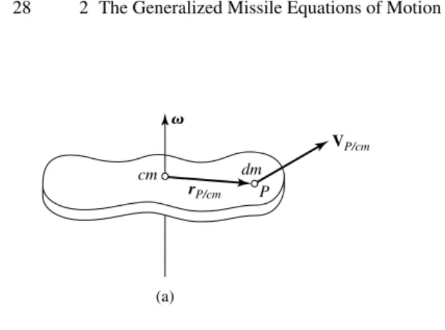
motion are obtained from Newton’s second law, which states that the summation of all externalforcesacting on a body is equal to the time rate of the momentum of the body, and the summation of the externalmomentsacting on the body is equal to the time rate of change ofmoment of momentum(angular momentum). Specifically, Newton’s laws of motion were formulated for a single particle. Assuming that the massmof the particle is multiplied by its velocityV, then the product

p=mV (2.15)

is called thelinear momentum. Thus, the linear momentum is a vector quantity having the same direction and sense asV. For a system ofnparticles, the linear momentum is the summation of the linear momenta of all particles in the system. Thus [8],

p=

n

i=1

(miVi)=m1V1+m2V2+ · · · +mnVn, (2.16)

whereidenotes theith particle, andndenotes the number of particles in the system. Note that the time rates of change of linear and angular momentum are referred to an absolute or inertial reference frame. For many problems of interest in airplane and missile dynamics, an axis system fixed to the Earth can be used as an inertial reference frame (see Figure 2.1). Mathematically, Newton’s second law can be expressed in terms of conservation of both linear and angular momentum by the following vector equations [1], [8], [11]:

F=d(mVM)

dt _I, (2.17a)

M=dH

dt _I, (2.17b)

wheremis the mass,Hthe angular momentum, and the symbol ]Iindicates the time rate of change of the vector with respect to inertial space. Note that (2.17a) is simply

F=dp

dt, (2.18a)

or

F=m _d_V

dt

=ma. (2.18b)

Equations (2.17a) and (2.17b) can be rewritten in scalar form, consisting of three force equations and three moment equations as follows:

Fx=

d(mu) dt , Fy=

d(mv) dt , Fz=

d(mw)