Mass transfer from a cylinder to an air stream in axisymmetrical flow (an experimental study)

· ....

STREAM IN AXISYMMETRICAL FLOW (AN EXPERIMENTAL STUDY)

Thesis by . Shiou-Shan Chen

In Partial Fulfillment of the Requirements For the Degree of

Doctor of Philosophy

California Institute of Technology Pasadena, California

1966

ACKNOWLEDGMENTS

The author wishes to express his sincere gratitude to

Professor B. H. Sage, without his inspiring guidance and constant encouragement this work would not have been completed at this time.

Appreciation is also due to H. T. Couch, W. M. Dewitt, G. Griffith, H. H. Reamer and H. E. Smith for their help in the construction and ope ration of the experimental equipment.

, Financial support in the form of Scholarships and Graduate \\

'

ABSTRACT

Mass transfer from wetted surfaces on one-inch cylinders with unwetted approach sections was studied experimentally by means of the evaporation of n-octane and n-heptane into an air

TABLE OF CONTENTS

INTRODUCTION . . . • . . . . THEORETICAL CONSIDERATIONS AND LITERATURE REVIEW • . . . . .

Differential Equations

.

.

.

.

Page 1

4 4

Laminar Boundary Layer 6

Transition . . .

9

Turbulent Boundary Layer . 13

Influence of Transverse Curvature 18

Heat Transfer vs. Mass Transfer 23

EXPERIMENTAL EQUIPMENT 25

Air Supply System 25

Porous Cylinder 27

Liquid Injection System 29

Measurement of Evaporating Surface Temperature 31

Local Velocity Measurement . . 33

MATERIALS AND THEIR PROPERTIES 34

N-heptane and N-octane 34

Air

EXPERIMENTAL RESULTS Flow Conditions

Velocity Distribution at Jet Opening Reynolds Number

Temperature of Evaporating Surface

TABLE OF CONTENTS (Continued)

Rate of Evaporation .

.

.

.

Sherwood Number

Remarks on Variable Physic::al Properties DISCUSSION OF RESULTS • . . . .

Influence of the Interfacial Velocity

Transition from Laminar to Turbulent Boundary Layer - . . . . Isothermal vs. Nonisothermal Evaporation Empirical Correlation of Experimental Data Comparison with Previous Work •

SUMMARY . . . NOMENCLATURE REFERENCES FIGURES TABLES

APPENDICES .

I. Liquid Loading System

II. Method of Averaging the Evaporating Surface Temperature . . . .

Page 43 44 46 47

47

49

59

69

94

Figure 1. 2. 3.

4.

6.

9.

16.

19.

20

.

LIST OF FI GU RES

Title

Hydrodynamic and Diffusion Boundary Layers Laminar and Turbulent Boundary Layers . . • Porous Cylinder, Air Jet, and Traversing Gear Air Supply System

Converging Air Jet

Cylinder Before Assembly Cylinder After Assembly Porous Section

Cylinder and Its Support

Liquid Injector and Associated Mechanism Liquid Injection System .

Traversing Thermocouple at Measuring Position Velocity Distribution in Air Jet at 1/4-in. Below Jet Opening, U

=

avg

Velocity Distribution in Air· Jet at 1/4-in. Below Jet Opening, U

=

avg

U /U as a Function of U

ro avg avg

Coordinate System . . . .

Experimental Results £or x = 1. 973 in. , x = O. 715 in. , n-heptane . 0 • • • •

w

Experimental Results for x = 1. 973 in. , 0

x

=

Experimental Results for x

=

x. = O. 500 in. , n-octane w

Experimental Results Uncorrected for Unwetted Approach Lengths . .

Figure 21. 22.

23.

24.

LIST OF FIGURES (Continued)

Title

Correlation of Experimental Data

Comparison of Results with Theoretical Work for Laminar Boundary Layer .

Comparison of Results with Previous

Measurements for Turbulent Boundary Layer Comparison of Results with Theoretical Work for Turbulent Boundary Layer

90

91

92

Table I. II.

III. IV.

v.

.

.

LIST OF TABLES

Title

Specifications of Heaters for Porous Sections Experimental Operating Conditions

Experimental Results

Range of Experimental Data

Comparison of Experimental Results Expressed >:C

in Sh:

1 and in Sh1 . . . .

95

96

98

106

INTRODUCTION

Mass transfer between a solid surface and a fluid is one of the most important subjects in chemical engineering. It occurs in many chemical engineering operations, such as drying, absorption, adsorption, extraction, heterogeneous chemical reactions (in

particular, surface catalytic reactions) etc. An understanding of mass transfer is therefore essential to the design and operation of process equipment. It is also important in the field of aero-nautical engineering in the study of problems such as ice formation

on aircraft and the maintenance of tolerable temperatures on the surface of high-speed aircraft by the use of transpiration cooling.

In most cases of industrial importance, the fluid flows relative to the solid surface and creates convective· mass transfer in addition to the molecular diffusion. It is therefore important to study the relationship between fluid flow and mass transfer or, more specifically, the dependence of mass transfer on fluid flow. Industrial mass transfer processes usually involve complex

equipment, and the basic principles of mass transfer are often complicated by the geometry and flow patterns. In order to

understand the .basic mechanism of mass transfer, it is desirable to study situations where boundary conditions are simple and well defined. The most frequently studied cases are flow past a flat plate (l, 2 • 3

>*;

parallel(S, 9 ) to the flow direction and, of course, flow in pipes(lO, ll)

(ll,12) and flow between parallel plates .

Axisymmetrical boundary layers occur in flows past axially

symmetrical bodies. The axisymmetrical case differs from the

two-dimensional case by including the effect of curvature in a

plane transverse to the flow direction. The influence of this

curvature on the values of local skin friction and thermal transfer

has been studied theoretically by Se ban and Bond(S} by considering

the problem of forced convection from a heated cylinder into the

surrounding axisymmetrical, incompressible, laminar boundary

layer produced by a uniform stream. No satisfactory theoretical

treatment is yet available for the corresponding turbulent boundary

layer case, and experimental work on this problem is lacking.

The purpose of the present investigation was to study

exp~rimentally the rate of mass transfer from a one-inch-diameter

porous cylinder to an air stream. The air stream flowed parallel

to the axis of the cylinder (axisymmetrical flow} and formed a

boundary layer along the surface of the cylinder. The boundary

layer was either laminar or turbulent depending on the flow

conditions. The porous section was preceded by an unwetted

length. There was no mass transfer between the unwetted

surface and the air stream, and thus the mass flux of the diffusing

component on the unwetted surface was zero. This unwetted length

is called the "approach length"(l3}.

section and raised by capillary force to form a thin film on the

porous surface. The Reynolds number was varied from 5, 000

to 310, 000 by changing the air velocity as well as the length of •

the approach section.

Two liquids, n-heptane and n-octane, were used as the

diffusing components. The difference in the vapor pressures of

these two compounds served to study the effect of the surface

concentration of the diffusing component on the rate of mass

transfer.

Both isothermal evaporation and non-isothermal e

vapora-tion were tested and the results were compared. The isothermal evaporation was achieved by supplying energy from a heater

located inside the porous section.

In summary, the following problems were considered in

the present investigation:

1. Dependence of the rate of mass transfer on the Reynolds

number.

2. Influence of the approach length on the rate of mass transfer.

3. Influence of the transverse curvature on the rate of mass

transfer.

4. Effect of the surface concentration of the diffusing component

on the rate of mass. transfer.

THEORETICAL CONSIDERATIONS AND LITERATURE REVIEW

Theoretical analyses relevant to this work are systematically

discussed in this chapter. For the convenience of comparing this work with measurements made by other investigators, previous

experimental results directly related to this work are reviewed. Analogies and differences among momentum, heat, and mass transfer will be discussed as the situation arises.

Differential Equations

For the case of two-dimensional, incompressible, steady fl.ow with negligible viscous dissipation, the boundary layer equations can be written as follows

continuity:

momentum:

energy:

8(pu) + 8{pv)

=

·

ax

ay

au

-8y

1 BTxy 1 8P

=

ay

-

'Pax

*

(2)

diffusion:

=

-1

p 8y

For the corresponding axisymmetrical case, the boundary layer

equations assume the following form

8(rpu} + 8(rpv} =

0

ax

au + au 1 8(r'T xr ) 1 BP

u - v -

=

8r

ax

ax

8T +v8T 1 8(rq ) r

u -

=

8r

ax

p

o(pk/p) +v

a(pk/p)

1 8(r~kr)

u

ox

8r

=

As is well known, no general solutions for the above

equations are available. It has been possible to obtain exact

solutions only for some simple problems such as laminar flow

fl 1 t · · d (l ' 2} A . h d

past a at p ate a zero inc1 ence . pprox1mate met o s

have been developed to solve more complicated situations. We

shall first discuss important results for the two-dimensional

case, which has been much better explored and usually gives a

good first approximation to the axisymmetrical case. The

(4)

(5)

(6}

influence of the transverse curvature on the transport processes

will then be discussed to illustrate the difference between the two-dimensional and axisymmetrical cases.

Laminar Boundary Layer

The momentum boundary layer equation was transformed

into an ordinary differential equation and solved exactly for

the case of flow along a flat plate at zero incidence by Blasius (l, 14}.

The local friction factor w-as fo"q.nd:to~he ·a fU.Ucti·or{ of the Reynolds .number as follows: ..

f

=

0.664

~Rex

(9)

The corresponding heat transfer problem for a flat plate with a constant wall temperature was first solved by Pohlhausen (3' lS}.

The rate of heat transfer was expressed in the form of the Nusselt number as a function of the Reynolds number and the

Prandtl number. The result can be approximated by the following formula with good accuracy

Nu

=

x x (10}

In the presence of an approach length the above equation

start at the same position as the momentum boundary layer, as shown in Figure 1. This problem was solved by Meyman ·{lb) and Eckert(l?) by substituting a

thir~-power

Nu

=

x x

1

(ll)

The function [ 1- (x

/n

inert approach length on the local Nusselt number and is called the "approach-length function. " The change of the surface temperature in the form of a step function is of practical im-portance. A solution to this problem opens the way to the

prediction of the heat transfer rates from surfaces of arbitrary temperature distribution by means of the principle of super-position, as one recalls that the energy boundary layer equation is linear. Methods for solving the problem of arbitrary tern-perature distributions along the surface of a flat plate have been given by Lighthill (l8), and Tribus and' Klein (l

9).

It is seen that when the plate is heated over its entire length, i.e. x = 0, Equation 11 reduces to the result of

0

Pohlhausen, Equation 10.

(12)

Equations 10 and 12 can also be derived from the Reynolds analogy

and the Blasius solution for momentum transfer for the special

case of Pr

=

For mass transfer with small solid-fluid interfacial

velocities; an equation analogous to Equation 11 can be derived

·,

{12)

If the entire length is maintained at a constant concentration,

Equation 12 becomes

Sh

=

o.

s~

/

Re

/

x . . x (13)

The mean Sherwood number is ·obtained by integrating the above

expression from x

=

=

(14)

The analogy between heat and mass transfer in this case

can be easily visualized since the energy boundary layer equation

(neglecting the thermal dissipation term) and the diffusion

is that for heat transfer the normal velocity at the wall is zero

but for mass transfer it is greater than zero. They should have

the same form of solution if the interfacial velocity in the mass

transfer case is sufficiently small.

The Colburn analogy also holds for laminar boundary layer

flow along a flat plate. The Colburn j-factors(20) are defined as

. - St p 2/3

Jh - h r

. =

st_z/

Jm m

for heat and mass transfer, respectively. A comparison of (15)

Equations 9, 10, 13, and 15 gives the following simple relation

(16)

The preceding formulas for heat and mass transfer are in good

agreement with the measurements of Elias <21

>,

Furber<22

>,

of heat from flat plates, and the measurements by Albertson (Z4}

for the evaporation of water from a flat plate ..

Transition

Since the celebrated experiment of Osborne Reynolds (lS)

classified into two basic hydrodynamic models, laminar flow and

turbulent flow. At low Reynolds numbers, fluids flow along

st~eam lines {laminar flow}. In this regime, mass transfer

in the direction normal to the flow depends only on the molecular

diffusion. When the Reynolds number is increased, the flow

undergoes a transition from the laminar to the turbulent regime,

where mixing of fluid particles in various directions takes

place. This macroscopic mixing is termed turbulence. In the

turbulent regime, macroscopic mixing dominates the mass

transfer process.

Since the mechanism of the transport process is distinctly

different in these two regimes, the transition from the laminar

to the turbulent flow is of fundamental importance in the study

of momentum, heat, and mass transfer. It is a well known fact

that for flow in a circular pipe, the transition occurs

approxi-mately between Re

=

The flow in a boundary layer can also undergo transition,

as shown in Figure 2. The process of transition in the

boundary layer on a flat plate with a sharp leading edge has

. db . . (26, 27, 28, 29, 30} N

been studie y many investigators . ear

·the leading edge the momentum boundary layer is always

laminar, but becomes turbulent further down stream. On a

flat plate with a sharp leading edge and in an air stream of the

level of turbulence of the order of 0. 5

%,

Re = 3. 5 X 10 5 to 10 6 x

Theoretical studies based on the method of small disturbances

indicate that the point of instability of a laminar motion takes

.1 t(l,31,32)

pace a

or

*

u

(

~

Re .

=

x, cr1t (

U00x )

=

6.

x 10

v . cr1t

for the boundary layer on a flat plate at zero incidence. At

Reynolds numbers larger than this value, some disturbances

may amplify themselves and make the laminar flow unstable.

This point of instability (or the theoretical critical Reynolds

number) gives the lower limit of the point of transition (or

experimental critical Reynolds number).

The point of transition depends strongly on the experi

-mental conditions. Using a special wind tunnel with a level of

turbulence lower than 0.1%, Dryden and his coworkers<33,34)

were able to maintain a laminar boundary layer for flow along

6

a sharp-edged flat plate up to Re = 2. 8 X 10 .

x They also

found that when the level of turbulence was lower than 0. 08%

further decreases in the level of turbulence did not increase

(17}

(18}

the critical Reynolds number. Accordingly, there seems to exist

an upper limit for the critical Reynolds number as well as a lower

limit. A comprehensive review on the transition from laminar

to turbulent flow has been given recently by Dryden (30}.

In many experiments where the angle of incidence was

not close to zero, transition at a Reynolds number of the order

4

of 10 was observed. This is pas sible since the point of

transition depends not only on the Reynolds number but also

on other parameters. The most important ones are the level

of turbulence of the main fluid flow, the pressure distribution

in the external flow, and the roughness of the wall. The lowest

Reynolds number employed in the mass transfer measurements

of Maisel and Sherwood(l3) was approximately 4 X 104, which

was already in the turbulent boundary layer regime. The heat

transfer measurements of Jacob and Dow(3S) for axisymmetrical

flow along a cylinder showed that the point of transition took

4 place at Reynolds number as low as 5 X 10 •

According to the Rayleigh theorem (3b), the velocity

pro-files which possess a point of inflection are unstable. The

pressure-distribution measurements by Sogin and Jacob<37) for

a cylinder with a hemispheric nosepiece in axisymmetrical

flow showed that there was a boundary layer separation

immediately after the hemispheric nosepiece, and consequently

there was a point of inflection. A hemispheric nosepiece will

turbulent boundary layer. This was experimentally verified by

Jacob and Dow<35). They used a hemispherical nosepiece and

a hemi-ellipsoidal nosepiece and found that in the former case

there was a lower value of the critical Reynolds number.

Turbulent Boundary Layer

The theoretical treatment of the laminar boundary layer

is rather straightforward, at least for flow along a flat plate,

and agrees well with the experimental results. The theoretical

analysis of the turbulent boundary layer has not been carried

out with such great confidence due to the complex nature of

turbulence which is not entirely understood. Mathematical

analyses of the turbulent flow always involve some semi-empirical

hypotheses. Since different investigators adopted different

hypotheses in deriving theoretical formulas, the results often

do not agree with each other. The agreement between

experi-mental measurements and theoretical formulas has not been as

good as in the laminar case. A detailed comparison of various

results has been given by Christian and Kezios (3B).

The classical method in the calculation of heat and mass

transfer in a turbulent boundary layer takes as its starting

point the Boussinesq expressions for shear stress and heat

flux (or mass flux) <39' l), and assumes that the ratio between

the shear stress and the heat flux, T

/q,

equal to a constant in the turbulent core. The resulting relation

between the temperature gradient and the velocity gradient is

then integrated to yield expressions for the heat flux. Additional

assumptions conce;i;-ning the velocity distribution across the

boundary layer have to be made when the integration is being

carried out. Consequently, different formulas have been

obtained by various investigators due to different assumptions

involved. The most widely accepted ones are those of

Prandtl (40) and Taylor<41

>,

>,

Rubes in <44). For the Prandtl number close to unity, the

for-mulas by Prandtl and by von Karman can be approximated by

the following simple expression with good accuracy(l)

Nu

=

x x

or

(20)

(21)

All the theoretical analyses indicate that the Nusselt number (or

Sherwood number, for mass transfer) is approximately

pro-portional to Re O. 8 for turbulent boundary layer along a flat

x

plate, provided the Prandtl number is not too far from unity.

A new theoretical method for the analysis of heat transfer

in a turbulent boundary layer has been developed recently by

Spalding(4S, 46• 47) by making use of the von Mises

identical with the one-dimensional diffusion equation in which the

coefficients are functions of the space coordinates. By assuming

proper forms of the universal law of the wall <49

>

turbulent Prandtl number .• the equation can be integrated

numerically to yield the heat transfer coefficient. This new

approach is more exact and elegant in the mathematical sense,

but the results are in the numerical form rather than the

analytical form obtained by the classical method. It is

there-fore rather inconvenient for practical applications. A survey

of the present status of knowledge concerning the transfer of

heat by forced convection across incompressible turbulent

boundary layers has been given by Kestin and Richardson (50).

The influence of the approach length on the rate of heat

transfer through a turbulent boundary layer was first studied

experimentally by Jacob and Dow<35). They..measured heat

transfer from a 1. 3-inch cylinder with a hemispheric nosepiece

in axisymmetrical flow for various approach lengths from 0. 07 5

to 1. 026 feet and a heated length of 8 inc.hes (x

0

/i.

5 6

Over a range of Re.e_= 2 X 10 to 1. 5 X 10 , the data were in

good agreement with the empirical relation

>'<

coefficient' by evaporating water from a flat plate into a turbulent

air stream for air velocities between 16 and 32 feet per second,

with wetted lengths of 2. 03, 4. 06, and 6. 09 inches, and approach

lengths of 5. 2, 10. 4, 20. 6, and 40. 6 inches. Over the range

4 5

of the Reynolds number from 6. 5 X 10 to 6. 5 X 10 , the data were

correlated by the following expression

with an uncertainty of ±15%. The approach-section functions

of Maisel and Sherwood, and of Jacob and Dow agree fairly well

for x

/i.

9.

differently as x

/i. -

*

1

+

o.

[

. 0 8]-0.ll 1 - (x

0/1} · . -oo

Maisel and Sherwood claimed that "In the present case x₀ is larger compared with xw; with the 5.1 cm. wetted section and 103 cm. approach section jm is essentially a point value and not an average over a wetted length 1. 11

This is certainly not true in view of the strong dependence of the mass transfer coefficient on x₀

/i.

Equation 23 .

(23)

(24}

Spielman and Jacob(5l) measured the mass transfer rate

from a flat plate by evaporation of water into an air jet and

concluded that the approach-section function of Maisel and

Sherwood gave a better correlation. However, their results are

somewhat doubtful in view of the high uncertainties (± 40%)

in-volved. It has been pointed out by Tribus (5l) in discussing

Spielman and Jacob's paper that the boundary conditions required

that the equation have a singularity at the point where the

tern-· perature or vapor pressure discontinuity occurred, therefore

the formula by Maisel and Sherwood was more realistic than

that of Jacob and Dow.

Theoretical formulas for the influence of the approach

length have been obtained by Se ban (SZ), Rube sin <53), and Reynolds

et al. <54). So far the experimental data are not extensive enough

. to make a clear choice among the various empirical and

theoretical formulas. This is also due to the difficulty that the

differences among the various formulas are of the same order

of magnitude as the uncertainties involved in most experimental

Influence of Transverse Curvature

The presence of curvature normal to the flow direction

affects the boundary layer structure, and hence the momentum,

heat, and mass transfer. In general, a transverse curvature

decreases the rates of heat and mass transfer in the case of

flow in a pipe (concave curvature); whereas for flow outside

an external surface, a transverse curvature (convex curvature)

increases the rates of heat and mass transfer. This can be

physically visualized since in the former case the sur~ace

area normal to the heat or mass flux decreases as it moves

away from the solid-fluid interface, and the situation is

re-versed in the latter case.

The boundary layer equations for the axisymmetrical

flow of a viscous fluid past a body of revolution were first

derived by Boltze(SS). Mil.likan(Sb) solved these equations by

using an approximate integral method and gave numerical results

for an airship movel. Since the Boltze formulation is based on

the assumption that the boundary layer thickness is much smaller

than the radius of the transverse curvature, the me~hod developed

by Millikan does not apply when the influence of the transverse

curvature on the structure of the boundary layer becomes

The influence of the transverse curvature on skin friction

and heat transfer in a laminar boundary layer from a cylinder in

axisymmetrical flow was first solved by Se ban and Bond(S) in the

form of series expansions in terms of the ratio of flat plate

displacement thickness to radius curvature. Important

numerical corrections to

thei~

and the resulting solution is referred to as the Se ban-Bond-Kelly

solution. For a Prandtl number of 0. 715, the result for heat

transfer can be expressed as follows

(Nux) cylinder

(Nux}plate

=

1+2.30(

~)Re

-l/2

a x . (26)

The leading term of the expansion is the corresponding flat plate

expression, and the subsequent terms are corrections for the

transverse curvature. Since the convergence of the solution is

poor as the boundary layer becomes thick, the solution is valid

only for the regime close to the leading edge of the cylinder. Since

then, Mark( 58), Stewarts on <59 ), and Glaue rt and Lighthill (bO}

have obtained approximate solutions by means of the momentum

integral method for the skin friction which cover the entire

range from weak curvature effects close. to. the leading edge of the

cylinder to strong curvature effects far downstream. Asymptotic

solutions for the heat transfer rate in the regilnes of strong and

moderate curvature effects have also been obtained by Bourne

effects of transverse curvature and mass injection have been

studied by Steiger and Bloom {63• 64

>,

The extension of the solutions to other bodies of revolution such

as cones and parabolas have been discussed by Yasuhara (66) and

Raat( 9 ). Christian and Kezios (3S) measured the rate of mass

transfer by sublimation from the outer surface of a hollow

naphthalene cylinder in a parallel air stream. Their data indicated

a smaller effect of curvature than any of the theoretical results

discussed above. However, the range of their measurement

was not extensive enough to lead to a decisive conclusion,

particularly in view of the soundness of the theoretical analyses.

The picture for the turbulent boundary layer is still very

obscure. No rigorous theoretical analysis is available. Most

measurements in heat transfer from bodies of revolution in

axisym-metrical flow have been carried out with large objects at high flow

speeds by aeronautical engineers. Due to the small boundary

layer thicknesses and large radii of curvature involved, little

information concerning the influence of the transverse curvature

on the rate of heat transfer has been gained from those

measure-ments <67). Theoretical analyses have been limited to approximate

methods based on a number of assumptions which have been

justified neither theoretically nor experimentally. Experimental

studies have not been satisfactory due to the fact that experimental

uncertainties involved in turbulent heat and mass transfer a:i;e

usually of the same order as the effect of the transverse curvature.

Jacob and Dow(3S) derived an expression for the influence

of transverse curvature on the rate of heat transfer by means

of an approximate integral method. In carrying out the integration

they assumed that for both the flat plate and the cylinder the 1/7-th

power velocity distribution law holds, and that the boundary layer

thickness is the same on the cylindrical surface as on a plane for

equal Reynolds numbers. This leads to the following result

( Nui)_ cylinder

(-Nui), plate

0

=

1+o.3

The thickness of the turbulent boundary layer,

o,

from the 1/7-th power law,

o

x (28)

Since the influence of curvature is a second-order effect (in com:..

parison with the first term which corresponds to heat transfer

from a flat plate), the use of an approximate method which involves

a number of unverified assumptions may give poor results. This

can be seen when one uses Jacob and Dow's method to evaluate the

influence of curvature on the heat transfer rate in a laminar

boundary layer. This leads to

( Nux) cylinder

(

Nux~

= 1

+

~)

A comparison of Equation 29 and the exact Seban-Bond-Kelly

solu-tion, Equation 26, shows that the influence of curvature obtained

by Jacob and Dow's method is almost twice the exact solution.

Another weak point of Equation 27 is that its convergence is poor.

From Equations 20, 27, and 28_, one obtains the following expression

for heat transfer from a cylinder

q t -t

s a

·U 0 8

=

1

..

u

1

+

o.

~)

0.2 x

0.8 x

--

= 0. 0296 kPrl/3

\~co)°"

:O.

2

+

(,:n

·

6

]

(30}

The l/x0· 2 term, which corresponds to the heat transfer from a

flat plate, indicates that the local coefficient decreases with

increasing x, as expected. But the second term, which is

pro-portional to x0· 6, increases with x at a much higher rate and

may overcome the decrease in the first term when the boundary

layer thickness reaches a certain high value. In other words,

the Jacob-Dow formula predicts that the rate of heat transfer at

first decreases with x, reaches a minimum, and then increases

with x. This phenomenon has never been observed experimentally

and is difficult to conceive physically.

A method which removes the assumption that the boundary

Landweber(bB) and H. U. Eckert( 69 ). The results are expressed

as the ratio of friction factors in terms of the boundary layer

thickness and cylinder radius

f 1/5

cylinder (l

+

.£ )

f =

3

plate

£cylinder

=

T

plate

1

+

o.

~

(1

+

.!.

.§.

The boundary layer thickness,

o,

1/5 1 0 4/ 5

o

+

3

a )

which is obtained by the momentum integral method and the 1/7 -th

power law.

(31)

(32)

(33) .

The skin-friction measurements of Chapman and Kester(70)

show that the influence of curvature is lower than the prediction of

the Jacob-Dow analysis and higher than the prediction of the

Landweber-Eckert analysis. No conclusion can be made from their

experimental results concerning the relative merits of these two

approaches.

Heat Transfer vs. Mass Transfer

Iri the above .discussions we have considered heat and mass

the energy and diffusion boundary layer equations have the same form. However, it should be pointed out that heat transfer and mass transfer are not exactly analogous since in mass transfer the normal velocity at the phase interface is not zero, rather t.he interface serves as a sink or source of the diffusing component.

This boundary condition makes the momentum boundary layer equation no longer independent but coupled with the diffusion boundary layer equation. The diffusion of a second component from the interface to the fluid (or vice versa} directly affects the boundary layer structure. In heat transfer the interfacial

velocity remains zero. Temperature variations across the

boundary layer can only change the velocity profile in an indirect way, namely by changing the properties of the fluid. When the temperature gradient is not very high, the momentum boundary layer equation can be treated independently of the heat transfer process.

Acrivos (7l) has developed asymptotic expressions for mass transfer in laminar boundary layer flows in the two-dimensional

EXPERIMENTAL EQUIPMENT

The principal parts of the equipment employed in this study

were the porous cylinder, the liquid injection system, and the air

supply system. Auxiliary equipment included devices for

measuring temperature and humidity, pitot tube, and

micro-manometers.

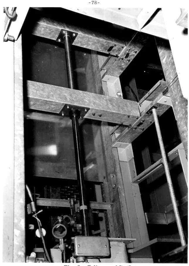
The one-inch porous cylinder with a hemispherical

nose-piece was placed vertically above a square air jet. Liquid was

supplied to the porous surface at predetermined rates from an

injector. A photograph of the experimental equipment is shown

in Figure 3.

Air Supply System

Figure 4 shows a schematic diagram of the air supply system.

The equipment used in this work was essentially the same as that

described by previous investigators in this laboratory(7' 7 2), except

that a square jet was used instead of the original' rectangular jet.

This open-circuit air tunnel was originally designed by Sage and

coworkers for the measurement of heat and mass transfer rates from

liquid drops, metal and porous spheres, at average air velocities

from 4 to 32 feet per second at the opening of the converging jet.

Air was pressed by two blowers, A, over wire grid heaters,

B, through a Venturi meter, V, into a system of 12-inch square

opening. The air blowers were driven by a direct current motor.

A glass-fiber filter was installed at the air inlet to the blowers

to provide clean air to the system. The bends in the ductwork

were equipped with vanes to reduce disturbances to the air stream

due to sudden changes in the flow direction. The smoothly

con-verging jet, shown in Figure 5, with a nozzle-contraction ratio

of 4. and the screens at the bottom of this section, S, were used

to reduce turbulence to a low· value in the test region. They also

provided a re!atively flat velocity profile at the jet opening.

According

~o

<

>,

leaving the converging jet was approximately 1. 3%.

The duct and the converging section were provided with

heaters which could be regulated independently to control the

temperature of the air stream. The reader is referred to

. {74) .

Corcoran et al. for details of the temperature control system.

Nine 36-gauge copper-constantan thermocouples were

located in the duct and jet to measure the temperature. The air

temperatures at the Ven~uri meter and at a point upstream of the

converging section were determined by means of platinum

resistance thermometers, shown at D and E, respectively, in

Figure 4. The resistance of the platinum resistance thermometers

was measured with a Mueller bridge, and the e.m.f. produced

by the thermocouples was determined with a White potentiometer.

The cold junctions of the thermocouples were maintained at the

by comparison with a standard platinum resistance thermometer

which was calibrated by the National Bureau of Standards.

The pressure difference across the Venturi meter was

used to establish the mass rate of air flow th1·ough the system,

Kerosene and mercury manometers along with a precision

cathetometer were used in the Venturi measurement. The

moisture content in the air was measured by means of

wet-and-dry bulb thermometers.

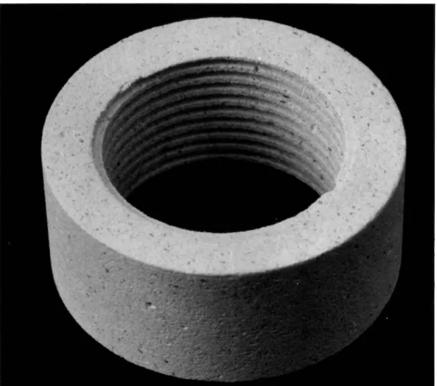
Porous Cylinder

The cylinder is shown in Figure 6 before assembly and in

Figure 7 after assembly. It consisted of an approach section, a

porous section, and a downstream section. All parts, with the

exception of the porous section, were made of brass. The porous

·section was made of medium.:: grade diatomacious earth

manu-factured by the Allen Filter Corporation.

Four different lengths of approach section of 1. 973, 4. 973,

9. 973, and 19. 973 inches were used. By using different approach

lengths, the Reynolds number could be varied independently of

the air velocity and the influence of the approach length on the rate

of mass :transfer could also be studied.

Two porous sections of O. 500 inch and 0. 715 inch were

tested. The O. 500-inch porous section is shown in Figure 8.

become rounded. Though extreme care was taken during the

machining and assembling, a discontinuous line with a width and

depth of approximately 0. 002 inch still existed between the approach

section and the diatomacious earth. Fortunately, when liquid was

fed into the porous earth, the liquid on the surface smoothed out

this discontinuity.

Isothermal mass transfer was achieved by supplying energy

from a heater coil placed in the helical grooves shown in Figure 8.

The use of a coil instead of a straight wire provided more uniform

heating and also made the assembly easier. The detailed

specifi-cations of the heater are described in Table I. The energy required

was supplied by 6-volt batteries. A resistor was used to adjust

the energy input to the heater.

The 18-inch downstream section provided a smooth air

stream after the porous section and thus prevented deformation

.

.

of the external flow by the cylinder support, shown in Figure 9.

The 3-inch gutter which supported the cylinder from the top also

contained the liquid line and the electrical wires. The downstream

section had an inner passage of 1/8-inch diameter, which served

as the liquid-supply line to the porous section. The thermocouple

and heater leads were also passed through this passage.

The cylinder was carefully positioned so that the cylinder

axis and the jet axis were on the same line. It was believed that

the angle of attack was less than five tenths of a degree. This

as previous investigators(70) already showed that the skin friction

was independent of the angJe of attack variations up to the order of

one degree.

Liquid Injection System

The evaporating component was supplied to the evaporating

surface at a predetermined rate from a liquid injector. A method

of cont.rol of a predetermined flow rate developed by Reamer and

Sage<7 5 ) was employed. Figure 10 shows a photograph of the

injector and some associated mechanisms. The speed of the

motor which drove the injector was controlled by a quartz oscillator

and a preset counter. For the details of the control circuit, the

reader is referred to the original paper by Reamer and Sage. The

liquid in the injector was maintained at a constant temperature of

100°F by means of an oil bath.

The liquid rate was so controlled that the evaporating

surface was completely covered by a very thin liquid film, but no

excess liquid was accumulated on the surface. In other words,

the liquid injection rate was equal to the rate of evaporation at

the porous surface. The attainment of this steady state was

determined with a manometer with a small diameter of O. 025 inch.

Figure ll shows schematically the liquid feeding system.

Due to the rather small capacity of the injector (20 cc.), a large

liquid sample to the evaporating surface when no reading was

being taken. The liquid level in the reservoir usually dropped

by less than 3 mm. during a test period of one hour. The

relatively constant liquid level and the fact that liquid was raised

to the evaporating surface mainly by the capillary force enabled

the maintenance of a constant flow rate from the reservoir to

the evaporating surface and kept the system at a steady state.

The liquid level (relative to the porous section} in the large

reservoir could be adjusted conveniently by a traversing gear

which moved the reservoir in the vertical direction.

As shown in Figure 11, two manometers were used.

Manometer ~· which was taped close to the porous cylinder,

was used to determine the correct injection rate as de scribed

above. The second manometer M

2, which was taped close to

the reservoir R, was used along with ~ to determine the

pressure drop of the liquid from the reservoir to the cylinder.

The difference in the liquid levels in ~ and M

2 provided an

approximate value of the flow rate from which one could estimate

the injector speed to be used.

The whole liquid injection system was evacuated by means

of a vacuum pump before it was filled with liquid. This ensured

that the liquid in the system was free of air bubbles. The liquid

sample was purified and deaerated before adding to the injector

and the reservoir. To avoid the accumulation of impurities on the

with purified sample. When no test was being made, a test tube

was used to surround the porous surface. The slight loss of liquid

.due ·to diffusion. into the stagnant air was continuously compensated

by filling from the reservoir. The rather tedious liquid filling

process did not have to be repeated unless leakage was discovered.

Measurement of Evaporating Surface Temperature

The measurement of surface temperature is always an

important and difficult matter in heat and mass transfer experiments.

In heat transfer, the temperature difference between the

solid-fluid interface and the free stream is used directly to establish

the heat transfer coefficient. In mass transfer,· due to the strong

dependence of vapor pressure on temperature, accurate

measure-ment of the surface temperature is equally important. The

depend-ence of the vapor pressure on temperature for the samples used

in this experiment was not as strong as for most liquids, such as

water, but still amounted to 2. 5% for n-heptane and 2. 8% for

n-octane, per degree Fahrenheit. The evaporation of a liquid on

the porous surface essentially formed an energy sink at the

inter-face, which established a large temperature gradient at the

neighborhood of the evaporating surface. This made accurate

measurements even more difficult. The position of the

thermo-couple became a very important problem in this experiment.

The direct extension of thermocouple wires from the inside

of the cylinder to the outer surface would not be satisfactory for

two reasons. First, it is difficult to locate the junction at the

correct position. Secondly, the large temperature gradient inside

the porous earth would affect the reading of the thermocouple.

The thermocouple wires must travel through a distance of a

constant temperature region before they reach the junction in

order to obtain accurate measurements.

During the construction of the porous cylinder, O. 003-inch

copper and constantan wires were passed from the inside of the

cylinder and extended to the surface at an angle of 456. The

wires traveled through an equal distance on the surface to meet at

the junction which was soft soldered. A groove had been cut

beneath the wires so that about one half of the wire diameter

was under the surface. With this arrangement, the error in

the temperature reading due to the heat conduction along the

thermocouple wires was essentially eliminated. This fixed

thermocouple was located midway between the edges of the porous

section.

The thermocouple as arranged above was not sufficient to

determine the surface temperature. The temperature of the

evaporating surface varied in the flow direction due to different

local evaporating rates and due to heat conduction between the

porous section and the neighboring parts. It was necessary to

use a traversing thermocouple to measure the surface temperature

averaged to obtain the surface temperature to be used in the

calcu-lation of the experimental results.

Figure 12. shows the traversing thermocouple and its probe

at a measuring position. When a reading was beiJ'lg taken, the

thermocouple was pressed against the porous surface to form an

arc. This provided isothermal regions on both sides of the junction

to minimize errors due to heat conduction along the wires. The

traversing thermocouple was also made of 0.003-inch copper and

constantan wires. The thermocouple probe was mounted on a

traversing gear, which located the position of the thermocouple to

within 0. 001 inch in the direction of the axis of the cyl~nder.

Local Velocity Measurement

Local velocities were measured by means of a pitot tube and

a micromanometer. The micromanometer was attached to a

traversing mechanis.m which was able to determine the vertical

MATERIALS AND THEIR PROPERTIES

N-heptane and n-octane

N-heptane and n-octane were chosen as the diffusing com-ponents for the following reasons:

1. Their vapor pressures at room temperature are typical in many

chemical processes. They are of the same order as the vapor

pressure of water. The use of hydrocarbons instead of water also avoids the uncertainties involved in the measurement of the moisture content in the air stream.

2. The dependence of their vapor pressures on temperature is small compared to other compounds. This reduces the experi-mental error due to the uncertainty involved in the measurement

of the temperature of the evaporating surface.

3. Physical properties required for the correlation of experimental -. data are available ~n the literature.

4. High-purity samples can be obtained at relatively low cost. 5. Small amounts of the sample present in the air do not give any

unpleasant odor or harmful affects.

The samples used were pure-grade n-heptane and n-octane obtained from the Phillips Petroleum Company. They had purities better than 99% according to the manufacturer. The sample was

first distilled through a laboratory-scale distillation column before

esti-mated purity greater than 99. 8%. The 0. 2% impurities probably

introduced little error to the final experimental results due to

the fact that they have approximately the same vapor pressure and

molecular weight as the main component. Therefore, for the

purpose of this work the samples could be considered as pure

substances.

The properties of n-heptane and n-octane used in correlating

the experimental data were as: follows:

1. Vapor Pressures: The vapor pressures were calculated

from the Antoine equations and the constants given by Rossini(76)

for .n-heptane:

for n-octane:

log p _{=A- C+t} B

A= S.21016

B = 2439. 227

c

=

A

=

5.

B = 2282. 607

c

2. Diffusivities: The diffusivity of n-octane in air was

calculated from the following equation taken from the International

. (77)

-4 ' T )2.00(.14.696 '

DF,k=l.1274Xl0 _{( 428}

p

)

The diffusivity of n-heptane in air was taken from the data of

Schlinger

.s:.!

. 1. 64 .

D = 0 8336 X 10 -4 (

l )

I

F, k . 560 \ P

for 520°R :5 T < 660°R.

3. Specific Volumes: The specific volumes of liquid

n-heptane and n-octane were taken from Rossini{76). At l00°F

and 1 Atm.,

Air

v

v

o.

for n-heptane

for n-octane

Air was considered as a single component in this work since

its composition was uniform. The specific volume of air was

calcu-lated from the pressure, temperature and humidity. The viscosity

EXPERIMENTAL RESULTS

Flow Conditions

The first step during each test was to bring the air stream to the desired flow rate and temperature. In order to ensure the steady-state operation of the equipment during the course of the measurement, the air fl.ow was started at the desired velocity about 4 hours before data were taken. During the stabilization period, measurements of the temperatures in the air duct and jet and of the pressure difference across the Venturi were made periodically. Those measurements along with the atmospheric pressure, room temperature and humidity measurements· were used to establish the flow rate. The average air velocity at the jet opening was calculated from the following equation

u

illa.

= p : - · p -

The weight flow rate and average velocity were not directly used to evaluate the Reynolds number, but were important for the establishment of flow conditions. The measurements of the flow conditions were made also before and after each test to ensure that steady-state conditions were maintained throughout the test period. Table II presents the conditions under which the experimental data were taken.

air flow was kept within O. 3% of the desired value throughout each

test. The average velocity ranged from 4 to 32 feet per second.

Velocity Distribution at Jet Opening

Although the smoothly converging jet with a high

nozzle-contraction ratio and the turbulence-damping screens succeeded in

providing a flat velocity profile at the opening of the air jet, the

velocity of the air stream at the central core was considerably

higher than the average velocity measured by the Venturi meter.

This was inevitable because the flow of a viscous fluid requires

that the velocity at the wall be zero. Consequently, there were large

velocity gradients close to the wall.

The velocity distribution in the air jet was measured by using

a pitot tube at a plane 1/4 inch below the jet opening. The results

for the average velocity at 32 and 8 feet per second are shown in

Figures 13 and 14, respectively. The velocity at the central core

was 4. 5% higher than the average velocity measured by the Venturi

meter at an average velocity of 32 ft/sec, and 14. 5% at 8 ft/sec.

We shall call the air velocity at the central core of the jet as U 00

for reasons to be discussed in the next section. Figure 15 shows

the values of U /U as a function of the average velocity. The oo avg

dotted line represents extrapolated values. Higher flow rates gave

flatter velocity profiles as expected.

The velocity distributions were integrated over the entire

The average velocity obtained by integration agreed with the

Venturi measurement to within 0. 5% for U

=

avg

for U = 8 ft/sec. The deviations mainly resulted from the

avg

difficulty in measuring velocities at positions close to the wall.

The velocities at the corners of the square jet were very low.

This phenomenon was also observed by Prandtl (30) and Nikuradse (3l}.

Reynolds Number

Since the boundary layer thickness for flow along a plate

or a cylinder increases in the flow direction, the correct length

parameter should be the distance along the interface from the

stagnation point as has been verified both theoretically and

experimentally(l}. In this work, the Reynolds number will be

defined as

Re1

=

u

-

--

where 1. is the sum of the approach length and the. wetted length,

1.

=

+

0

w

equal to the length of a cylindrical section with the same external

surface area. For a hemispherical nosepiece, this equivalent

length happens to be equal to its radius. Figure 16 shows the

relevant coordinate system used in this work.

The air stream which emerged from the air jet had a nearly

in Figures 13 and 14. During each test, a pitot tube was placed

parallel to the cylinder axis just outside the boundary layer at the

wetted section to measure the velocity of the external flow. It

I

was found that this velocity, U

00, was essentially independent of

the distance from the jet opening, except for the test made at

x _{o .} = 19. 973 inches and U _ro = 8. 93 ft/sec. During that test it was found that the velocity at the edge of the boundary layer was

3% lower than the correct value. When a thermocouple was

placed in the boundary layer, temperature fluctuations larger

than 1°F were observed. It appeared that an interaction between the boundary layer on the wall and the free jet ·mixing. region occurred in this particular test. This was not observed in other tests. The boundary layer on the cylinder wall remained well within the potential core of the free air jet, with the one exception

just mentioned, and the velocity of the external flow could be taken as equal to the air velocity at the potential core leaving the

con-verging jet.

A series of three or more tests was made at different air

velocities at a fixed approach length. After the completion of each

series of tests, the approach section was changed to a different

length and the position of the cylinder was readjusted to ensure ,,

that the stagnation point was at the jet opening.

Temperature of Evaporating Surface

When the air flow was adjusted to the desired conditions and

remained steady-state, the test tube surrounding the porous section

was removed and electric energy was supplied from the batteries

to the heater inside the porous section. One or two 6-volt batteries

were used depending on the rate of evaporation. Usually, it took

30 to 60 minutes for the surface temperature to reach a steady

value of l00°F as indicated by the fixed thermocouple at the middle

of the porous section. Suitable adjustment of the resistor kept

the surface temperature to within 0. 1°F of the desired value for

the duration of the test being carried out.

Tests'; were also made without energy supply from the heater

inside the porous section. Under this condition, the energy

required for the evaporation of the liquid from the porous surface

came from the air stream and the neighboring parts in contact with

the porous section. When steady- state conditions were reached, the

surface temperature was 10 to 15 degrees lower than the tempera

-ture of the main air stream, depending on the rate of evaporation

and the position of the porous section. These tests will be referred

to as 11

nonisothermal evaporation, 11

and the tests made under

nearly-isothermal conditions will be referred to as "isothermal

evaporation. "

Immediately after the evaporation rate was determined,

temperatures at 9 or more points along the porous surface in the

thermo-couple for the purpose of evaluating the average surface tempera

-ture. The method of evaluating the average surface temperature

is described in Appendix II.

The traversing thermocouple agreed with the fixed thermo

-couple to within 0. 2°F when they were within 0. 005 inch. This

indicated that the temperature measurement by the traversing

thermocouple was reliable. It was also found that the presence of

this traversing thermocouple did not have any appreciable influence

on the rate of evaporation of the liquid. In other words, the

thermocouple did not affect the boundary layer to a degree sufficient

to introduce errors to the measurement. Tests were made to

determine the dependence of the average surface temperature on

the angular positions. The difference in the ave rage surface

tem-perature at different angular positions had a maximum of only

0

0.1 F, and could be neglected for practical purposes.

In spite of all the precautions, the uncertainties involved in

the measurement of the evaporating surface temperature probably

contributed the major share of errors to the final experimental

results, due to the inherent difficulties. It was estimated that the

uncertainty in the average surface temperature was probably up

to 0. 4°F, mainly due to the errors in the measurement and in the

averaging process .

Rate of Evaporation

After the air flow, evaporation rate, and evaporating surface temperature had reached steady-state conditions, the

liquid injector was started at c~ s:p~}ed esti:tnatcd from the pre$sU:re drop between the liquid reservoir and the porous cylinder shown in Figure ll. The valve to the reservoir was then closed. The liquid level in Manometer M

1 was used as an indicator for

adjusting the liquid injection rate to the correct value by means of the preset counter. The measurement was continued for

approximately 20 minutes to ensure that the injection rate was correct and that the experimental conditions were steady. The preset counter as: well as the fixed thermocouple were read at about 3-p:linute intervals. They agreed exactly except when mechanical or electronic failures occurred. At the end of the

measurement the valve to the liquid reservoir was opened and the injector was re-filled with liquid from a liquid loading system described in Appendix I.

It was observed that when the liquid rate was at the vicinity of the desired value, the liquid level in Manometer M

level in the manometer would drop by more than 1 cm. This

sensitive method provided an accurate measurement of the injection

rate. It appeared that when the liquid sample was injected at the

correct rate, the evaporating surface was completely covered by

a. very thin liquid film but no excess liquid was accumulated on

the surface. This phenomenon is independent of the porosity of

the porous material, provided that the material has a sufficiently

high porosity and the pore diameters are small enough to give a

r

:t:

high capillary pressure '

The results of this measurement are shown in Table III.

The reproducibility of the liquid rate measurement was better than

1%, with a few exceptions.

Sherwood Number

From the rate of evaporation, the surface temperature, and

physical properties of air and the diffusion substance, one can

calculate the Sherwood number from the following expression

{36}

t This method has been used by Sage and coworkers for

measure-ments of mass transfer rates from porous spheres. See, e.g.,

references (79) and (83).

:i:

of 1 micron, the surface tension will give a capillary pressure of

5 psi, which is sufficient to raise the liquid to a height of 15 feet

against the gravitational force . . This high capillary pressure

which is derived in detail in Appendix III. The logarithmic term

in Equation 36 results from the net flow due to the diffusion of one

component into a second component. We shall call the Sherwood

number defined by Equation 36 the 11

modi£ied Sherwood number"

since it does not come directly from the conventional definition.

The validity of this expression will be discussed in a later section.

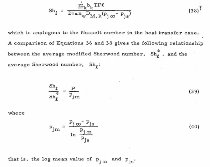
Equation 3 6 represents the average modified Sherwood

number because the average weight rate of evaporation was used

in the calculation. The partial pres sure of the diffusing component

at the solid-air interface was assumed equal to the vapor pressure

of the liquid at the interface.. The results of this calculation are also shown in Table III.

Theoretically, fugacity difference instead of partial pressure

difference may be the more logical choice as the driving force for

mass transfer(SZ). However, the concentration of the diffusing

component in this experiment was low, thus the difference between

the fugacity and the part1al pressure was small. The consistent

use of partial pres sure throughout this work should introduce few

errors. The use of partial pressure also comes from the practical

reason that diffusivities obtained from the literatur.e .. are based on partial pressure rather than the fugacity.

Remarks on Variable Physical Properties

Since the diffusion boundary layer was thin relative to the

momentum boundary layer and the concentration of the diffusing

component was small, the mass transfer process had little effect

on the boundary layer flow. The physical properties of the free

stream air were used to calculate the Reynolds number. On the

other hand, the Sherwood number and the Schmidt number are

directly related to the mass transfer process, and were therefore

evaluated at the mean temperature:

t

=

+

m a s (37)

The influence of the diffusing component on the kinematic viscosity

is not known and was neglected in the calculations •

DISCUSSION OF RESULTS

Influence of the Interfacial Velocity

The mass transfer problem differs from the corresponding heat 'transfer problem by the fact that the normal velocity at the phase boundary is not zero. The evaporation and transfer of a liquid into an air stream create an additional net flow in the gas phase. The chemical engineer usually incorporates this net

flow into the Sherwood number by considering the diffusion of a second component through a stagnant gas. With this method the average Sherwood number, which we call the average modified Sherwood number, can be expressed by Equation 36

t